An Infinite Set of Integral Formulae for Polar, Nematic, and Higher Order Structures at the Interface of Motility-Induced Phase Separation

Abstract

Motility-induced phase separation (MIPS) is a purely non-equilibrium phenomenon in which self-propelled particles phase separate without any attractive interactions. One surprising feature of MIPS is the emergence of polar, nematic, and higher order structures at the interfacial region, whose underlying physics remains poorly understood. Starting with a model of MIPS in which all many-body interactions are captured by an effective speed function and an effective pressure function that depend solely on the local particle density, I derive analytically an infinite set of integral formulae (IF) for the ordering structures at the interface. I then demonstrate that half of these IF are in fact exact for a wide class of active Brownian particle systems. Finally, I test the IF by applying them to numerical data from direct particle dynamics simulation and find that all the IF remain valid to a great extent.

1 Introduction

The study of active matter is crucial to our understanding of diverse living matter and driven synthetic systems [1, 2]. In addition to being paramount to our quantitative description of various natural and artificial phenomena, much novel universal behaviour has also been uncovered in active matter systems in the hydrodynamic limits, which ranges from novel phases [3, 4, 5, 6, 7, 8, 9, 10] to critical phenomena [11, 12]. Besides the hydrodynamic limits, interesting emergent phenomena also occur in the microscopic and mesoscopic scales. In the case of motility-induced phase separation (MIPS) [13, 14, 15, 16, 17], one of these emergent phenomena is the polar-nematic ordering behaviour at the liquid-gas interface (Fig. 1) [18, 19, 20, 21, 22]. Understanding this phenomenon will be integral to modelling quantitatively diverse interface-related properties of MIPS that include nucleation [23], wetting [24, 25], negative interfacial tension [26, 27, 28], and reverse Ostwald ripening [29, 30].

Although the interfacial ordering ultimately emerges from the many-body interactions of the particles, similar pattern in fact already occurs in a system of non-interacting self-propelled particles (i.e., an ideal active gas) around an impenetrable wall – particles stuck at the wall tend to point towards it (hence the system is polar), and particles right outside the wall are predominantly moving parallel to the wall (hence nematic), since they constitute particles whose orientations have just rotated enough to be pointing away from the wall [31, 32]. This revelation suggests that the polar-nematic pattern observed in MIPS can be studied using an effective model in which all particle-particle interactions are captured by a velocity field that depends purely on the system’s local configurations, such as the local particle density. Implementing this task is the goal of this paper. Specifically, I first derive the equation of motion (EOM) of the many-particle distribution function under the assumptions that the effective speed and the effective pressure depend solely on the local properties of the particle density. I then obtained the steady state equations that describe the polar, nematic, and higher order tensor fields of the system, and from these an infinite set of integral formulae (IF), one for each tensor field. Moreover, I test these IF on published numerical data obtained from direct particle dynamics simulation [18], and demonstrate that the IF remain valid to a remarkable extent. Finally, I showed in the appendix that half of the IF hold exactly for a wide class of active Brownian particle systems that exhibit MIPS.

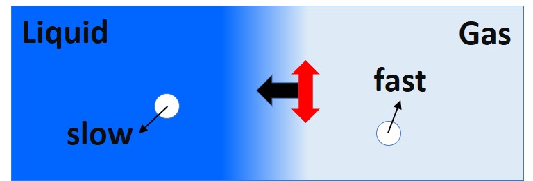
Figure 1: Schematic of the generic polar-nematic ordering observed at the interface of MIPS. The shade of blue depicts the particle density of the system. The particles’ orientations are isotropic in the bulks of both liquid and gas phases. As one approaches the interface from the liquid (condensed) phase, the average orientation of the particles at the interfacial region becomes predominantly polar (pointing towards the liquid phase as indicated by the black arrow), and then predominantly nematic (i.e., particles’ orientations tend be approximately vertical, as indicated by the red double-arrow.) Higher order tensorial structures beyond the polar and nematic fields also emerge at the interfacial region. Here, using an model in which the effective speed of the particles and the effective local pressure in the system depend solely on the local density, an infinite set of integral formulae is obtained for all these tensorial structures.

2 Effective model

In two dimensions, an archetype of active systems exhibiting MIPS consists of a collection of $N$ polar self-propelled particles in a finite volume $V$, such that the particles interact purely sterically via a short-ranged repulsive potential energy $U$, whose exact form is unimportant. Each particle also exerts a constant active force, $f_{a}$, that points to a particular orientation denoted by $\hat{\mathbf{n}}\equiv\cos\Theta\hat{\mathbf{x}}+\sin\Theta\hat{\mathbf{y}}$, and the angle $\Theta$ itself undergoes diffusion with the rotational diffusion coefficient $D_{\rm R}$. Furthermore, the particles can potentially perform Brownian motions characterized by the diffusion coefficient $D_{\rm T}$. Overall, the microscopic equations of motion (EOM) of the system are therefore

$$\frac{{\rm d}\mathbf{R}_{i}}{{\rm d}t} =-\frac{1}{\eta}\sum_{j\neq i}{\bf\nabla}_{\mathbf{R}_{i}}U(|\mathbf{R}_{i}-\mathbf{R}_{j}|)+\frac{f_{a}}{\eta}\hat{\mathbf{n}}_{i}+\sqrt{2D_{\rm T}}\mathbf{g}^{\rm T}_{i}(t)$$ (1a)

$$\frac{{\rm d}\Theta_{i}}{{\rm d}t} =\sqrt{2D_{\rm R}}g^{\rm R}_{i}(t)\ ,$$ (1b)

where the indices $i,j$ enumerate the particles ($i,j=1,2,\ldots,N$), $\mathbf{R}_{i}(t)$ is the $i$-th particle’s position at time $t$, $\eta$ is the damping coefficient in this overdamped system, and $\mathbf{g}^{\rm T}$’s and $g^{\rm R}$’s are independent Gaussian noise terms with zero means and unit variances, e.g., $\langle g^{\rm R}_{i}(t)\rangle=0$ and $\langle g^{\rm R}_{i}(t)g^{\rm R}_{j}(t^{\prime})\rangle=\delta_{ij}\delta(t-t^{\prime})$.

Since the particles’ identities are irrelevant, we can focus instead on the temporal evolution of the $N$-particle distribution function:

$$\psi(\mathbf{r},\theta,t)=\left\langle\sum_{i=1}^{N}\delta^{2}(\mathbf{r}-\mathbf{R}_{i}(t))\delta(\theta-\Theta_{i}(t))\right\rangle\ ,$$ (2)

where the angular brackets denote averaging over the noises.

As mentioned before, the goal here is to account for all particle-particle interactions and fluctuations effectively through a speed function and a pressure function that depend solely on the local density: $\rho(\mathbf{r},t)=(2\pi)^{-1}\int{\rm d}\theta\psi(\mathbf{r},\theta,t)$. Specifically, the model EOM of $\psi$ is assumed to be of the form:

$$\partial_{t}\psi=-{\bf\nabla}_{\mathbf{r}}\cdot\left(\mathbf{v}\psi\right)+D_{\rm T}{\bf\nabla}^{2}_{\mathbf{r}}\psi+D_{\rm R}\partial_{\theta}^{2}\psi\ ,$$ (3)

where $\mathbf{v}$ is the ‘velocity field’ taken to be

$$\mathbf{v}(\mathbf{r},\theta,t)=u(\rho(\mathbf{r},t))\hat{\mathbf{n}}(\theta)-\rho(\mathbf{r},t)^{-1}{\bf\nabla}P(\rho(\mathbf{r},t))\ ,$$ (4)

and $u$ and $P$ are the effective density-dependent speed and pressure functions, respectively. Note that the ‘effective pressure’ $P$ does not necessarily correspond to the mechanical pressure in a thermal system, or the Irving-Kirkwood pressure defined for passive systems [33]. Instead, $P$ should be viewed as a density-dependent scalar function whose spatial gradient contributes to the velocity field as described in Eq. (4). I further note that allowing the effective functions $u$ and $P$ to depend also on the spatial derivatives of $\rho$ (e.g., $\nabla^{2}\rho$) will not alter the key results here. In the Appendix, I will relate the approximation adopted here to a formally exact set of hierarchical EOM.

Given the model equations (3,4), we are now ready to systematically construct a reduced set of EOM in which the fields of interest depend on $\mathbf{r}$ and $t$, but not $\theta$. Specifically, these fields will be $m$-th rank tensors of the form:

$$T^{(m)}_{\alpha_{1}\cdots\alpha_{m}}=\frac{1}{2\pi}\int{\rm d}\theta\hat{n}_{\alpha_{1}}\hat{n}_{\alpha_{2}}\cdots\hat{n}_{\alpha_{m}}(\psi-\rho)\ ,$$ (5)

where the Greek letters enumerate the spatial coordinates and the subtraction of $\rho$ in the integrand ensures that these tensor fields vanish if $\psi$ is isotropic in $\theta$. For instance, the unnormalized polar field ${\bf M}(\mathbf{r},t)$ and nematic field $\mathbf{Q}$ are the first-rank and second-rank tensors, respectively:

$$M_{\alpha}=\frac{1}{2\pi}\int{\rm d}\theta\hat{n}_{\alpha}\psi\ \ \ ,\ \ \ Q_{\alpha\beta}=\frac{1}{2\pi}\left(\int{\rm d}\theta\hat{n}_{\alpha}\hat{n}_{\beta}\psi\right)-\frac{\rho}{2}\delta_{\alpha\beta}\ .$$ (6)

These fields are unnormalized since they are not normalized by the density, as opposed to, e.g., the normalized polar field ${\bf M}^{\rm N}=(2\pi\rho)^{-1}\int{\rm d}\theta\hat{\mathbf{n}}\psi$.

From (3,4), the EOM of the density and polar fields can be obtained:

$$\partial_{t}\rho= -\partial_{\alpha}\left[uM_{\alpha}-\partial_{\alpha}\left(P+D_{\rm T}\rho\right)\right]$$ (7a)

$$\partial_{t}M_{\alpha}= -\partial_{\beta}\left[u\left(Q_{\alpha\beta}+\frac{\rho}{2}\delta_{\alpha\beta}\right)-\frac{M_{\alpha}}{\rho}\partial_{\beta}P-D_{\rm T}\partial_{\beta}M_{\alpha}\right]-D_{\rm R}M_{\alpha}\ ,$$ (7b)

where $\partial_{\alpha}\equiv\partial/\partial r_{\alpha}$ and repeated indices are summed over. The EOM of higher order tensor fields can be derived similarly, as illustrated next.

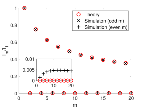
Figure 2: The integrals of the $m$-th rank tensor fields normalized by the integral of $M_{x}$ (denoted by $I_{1}$) (16). The analytical results are denoted by red circles (13c,15), and the corresponding integral values obtained using data from direct particle simulation are shown by black crosses (odd $m$) and black pluses (even $m$). The inset plot zooms into the $m$-axis to show the small deviations of the numerical results from the analytical predictions for even $m$.

3 Integral formulae at the steady state

I will now focus exclusively on the steady state in the phase separated regime, where there is a single liquid-gas interface located around $x=0$. By construction, spatial variations occur only along the $x$ direction, and we thus need only to consider tensor fields with all subscripts being $x$, i.e., tensor fields of the form $T^{(m)}_{x\cdots x}$. For later convenience, I will further denote $T^{(m)}_{x\cdots x}$ by $O_{m}$ when $m$ is odd and by $E_{m}$ when $m$ is even. Specifically, from the definitions of the tensor fields (5), we have

$$O_{m}=\frac{1}{2\pi}\int{\rm d}\theta\cos^{m}\theta\psi\ ,\ E_{m}=\frac{1}{2\pi}\int{\rm d}\theta\cos^{m}\theta\psi-K_{m}\rho\ ,$$ (8)

where

$$K_{m}\equiv\frac{(m-1)!!}{2^{m/2-1}m(m/2-1)!}\ .$$ (9)

At the steady state, the equations satisfied by the tensor fields are, from (3,4):

$$D_{\rm R}M_{x}= -\frac{{\rm d}}{{\rm d}x}\left[u\left(Q_{xx}+\frac{\rho}{2}\right)-\frac{M_{x}}{\rho}\frac{{\rm d}P}{{\rm d}x}-D_{\rm T}\frac{{\rm d}M_{x}}{{\rm d}x}\right]\ ,$$ (10a)

$$4D_{\rm R}Q_{xx}= -\frac{{\rm d}}{{\rm d}x}\left[uO_{3}-\frac{Q_{xx}+\rho/2}{\rho}\frac{{\rm d}P}{{\rm d}x}-D_{\rm T}\frac{{\rm d}Q_{xx}}{{\rm d}x}\right]\ ,$$ (10b)

$$D_{\rm R}\left[m^{2}O_{m}-(m-1)mO_{m-2}\right]= -\frac{{\rm d}}{{\rm d}x}\left[u\left(E_{m+1}+K_{m+1}\rho\right)-\frac{O_{m}}{\rho}\frac{{\rm d}P}{{\rm d}x}-D_{\rm T}\frac{{\rm d}O_{m}}{{\rm d}x}\right]\ ,\ \ {\rm for\ odd}\ m>1\ ,$$ (10c)

$$D_{\rm R}\left[m^{2}E_{m}-(m-1)mE_{m-2}\right]= -\frac{{\rm d}}{{\rm d}x}\left[uO_{m+1}-\frac{E_{m}+K_{m}\rho}{\rho}\frac{{\rm d}P}{{\rm d}x}-D_{\rm T}\frac{{\rm d}E_{m}}{{\rm d}x}\right]\ ,\ \ {\rm for\ even}\ m>2\ .$$ (10d)

The L.H.S. of (10) follow from the identities below:

$$\int{\rm d}\theta\cos^{m}\theta\partial_{\theta}^{2}\psi=\int{\rm d}\theta\left[(m-1)m\cos^{m-2}\theta-m^{2}\cos^{m}\theta\right]\psi\ ,$$ (11)

and for the L.H.S. of (10d), I have additionally used the identity:

$$m^{2}K_{m}-(m-1)mK_{m-2}=0\ ,$$ (12)

which can be readily derived from the definition of $K_{m}$ (9).

Since $\psi$ is isotropic in both $x$ and $\theta$ deep in the liquid and gas phase, $M_{x},Q_{xx},O_{m}$, $E_{m}$, and ${\rm d}P/{\rm d}x$ all vanish when $|x|\gg 0$. Therefore, by integrating both sides of (10) over the whole $x$ domain, we arrive at the followings:

$$\int_{-\infty}^{\infty}{\rm d}xM_{x}=K_{2}A= \frac{A}{2}\ ,$$ (13a)

$$\int_{-\infty}^{\infty}{\rm d}x\left[m^{2}O_{m}-(m-1)mO_{m-2}\right]= K_{m+1}A\ ,$$ (13b)

$$\int_{-\infty}^{\infty}{\rm d}xQ_{xx}=\int_{-\infty}^{\infty}{\rm d}xE_{m}= \ 0\ ,$$ (13c)

where

$$A\equiv\frac{1}{D_{\rm R}}\left[\lim_{x\rightarrow-\infty}u(\rho(x))\rho(x)-\lim_{x\rightarrow\infty}u(\rho(x))\rho(x)\right]\ .$$ (14)

In fact, one more simplification can be made: starting with (13a) and using (13b), one can readily prove by mathematical induction that

$$\int_{-\infty}^{\infty}{\rm d}x\langle O_{m}\rangle=K_{m+1}A\ .$$ (15)

The integral formulae (IF) expressed in (13c) and (15) are the key results of this paper. In the appendix, I will further show that for even $m$, the IF (13c) are in fact exact in a wide class of active Brownian particle systems.

Introducing the following notation:

$$I_{m}=\left\{\begin{array}[]{ll}\int{\rm d}x\langle O_{m}\rangle\ ,&m\ {\rm odd}\\ \int{\rm d}x\langle E_{m}\rangle\ ,&m\ {\rm even}\ ,\end{array}\right.$$ (16)

the plot of $I_{m}/I_{1}$ vs. $m$ is shown in Fig. 2 (red circles). Note in particular the slow decay of $I_{m}/I_{1}$ for odd $m$, which goes asymptotically to 0 as $m^{-1/2}$ (9).

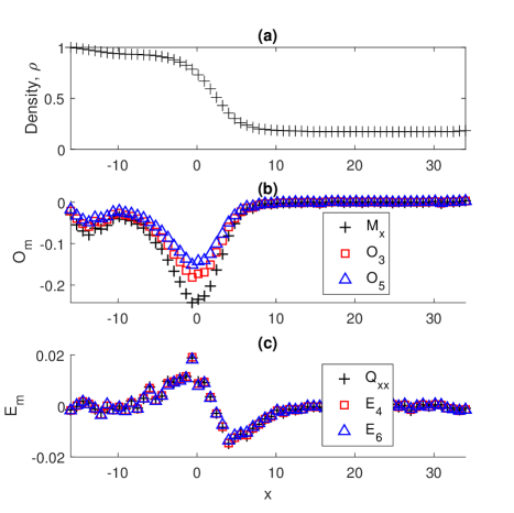
Figure 3: The variations of the density $\rho$ (a), the odd-rank tensor fields $O_{m}$ (b), and the even-rank tensor fields $E_{m}$ (c), with respect to $x$ at the steady state of a system of self-propelled particles with repulsive interactions that exhibits MIPS. The simulation data used for these curves are from a previous study [18].

4 Testing the integral formulae on a microscopic model of MIPS

As a test of the validity of the IF to realistic active systems exhibiting MIPS, I now re-analyse the numerical results obtained from simulating a microscopic model of MIPS [18]. Specifically, the simulation is on a system of 300 particles confined in a 2D channel of height $10\sin(\pi/3)$ and length $50$. A periodic boundary condition is used for the vertical direction, a hard wall is placed on the left of the channel, and particles exiting the right wall will stay at the right wall but with its orientation randomized. These particles interact via short-ranged repulsive interactions in the form of the Weeks–Chandler–Andersen potential [34]:

$$U(r)=\left\{\begin{array}[]{ll}\frac{26}{6}\left[\frac{1}{r^{12}}-\frac{2}{r^{6}}+1\right]\ ,&{\rm if}\ r<1\\ 0\ ,&{\rm otherwise}\ .\end{array}\right.$$ (17)

Other parameters are: $\eta=1,f_{a}=100,D_{\rm T}=0$, and $D_{\rm R}=3$.

At the steady-state, the density and various tensor field profiles are shown in Fig. 3. Given that the liquid phase is on the left (Fig. 3a), the odd-rank tensor fields $O_{m}$ are all negative around the interface (Fig. 3b), as the particles’ orientations are mostly pointing towards the liquid phase (black arrow in Fig. 1). For the even-rank tensor fields $E_{m}$ (Fig. 3c), they first become positive when approaching the interface from deep in the liquid phase, indicating that their orientations are predominantly horizontal, consistent with the orientation of the polar field. These fields then subsequently become negative as one exits the interface, indicating that the particles’ orientations become predominantly vertical (red double arrow in Fig. 1). The “oscillatory” feature of $E_{m}$ around the interface is of course necessary in order for the overall integrals of $E_{m}$ to be zero (13c). Note also that while all tensor fields go to zero as $m$ goes to infinity, they apparently do so rather slowly (Fig. 3(b)-(c)). This is again consistent with the analytical result that $I_{m}\sim m^{-1/2}$ for odd $m$. Overall, this slow decays indicates that a quantitative theory focusing on the interfacial region will need to incorporate a large number of higher order tensor fields. Finally, performing the integrals to this set of data as prescribed in (16), the numerical result (black crosses and pluses in Fig. 2) demonstrates that the IF are indeed valid to a great extent.

5 Summary & Outlook

Starting with a generic microscopic model of active particle system with only repulsive interactions, and adopting the simplifying assumptions that all many-body physics and fluctuations can be captured by an effective speed function and an effective pressure that depend solely on the local particle density, I have derived a set of EOM that describes the polar, nematic, and higher order tensor fields of the system. Focusing then on the steady state with a single liquid-gas interface, I obtained an infinite set of IF, one for each tensor field. I then tested these IF on data obtained from direct particle dynamics simulation of a microscopic model of MIPS, and found that the IF remain valid to a high accuracy. Furthermore, I showed in the appendix that half of these IF (even $m$) are in fact exact for a wide class of active Brownian particle systems. The overall validity of all the IF suggests that the model assumptions are appropriate when studying interfacial properties of MIPS.

This work opens up a number of interesting future directions: (1) For finite systems, the IF can be made more precise by incorporating the exact boundary conditions at the two limits of the spatial integrals. (2) The IF can be readily modified to sum rules for lattice models of MIPS [35, 36, 37, 38]. (3) It would be interesting to consider how these IF can be generalized to a system of active particles with alignment interactions. Indeed, the various types of travelling bands observed in polar active matter [39, 40, 41, 42, 43, 44, 45, 46, 47, 48, 49] are reminiscent of the soliton solutions in the Korteweg–De Vries equation, which also admits an infinite number of integrals of motion. (4) Finally, the analytical treatment here provides a basis for developing a quantitative theory that elucidates how the interfacial ordering impacts upon other interface-related phenomena in MIPS, such as the Gibbs-Thomson relation [18], wetting [24, 25], and reverse Ostwald ripening [29, 30].

Appendix A Relating the approximation to an exact hierarchical EOM

In this appendix, I will relate the key approximation made in the main text to a formally exact set of EOM of the tensor fields. To do so, I will start with the fluctuating $N$-particle distribution function:

$$\psi^{(f)}(\mathbf{r},\theta,t)=\sum_{i=1}^{N}\delta^{2}(\mathbf{r}-\mathbf{R}_{i}(t))\delta(\theta-\Theta_{i}(t))\ ,$$ (18)

where the superscript $(f)$ specifies that $\psi^{(f)}$ is a fluctuating quantity (hence different from $\psi$ (2)) due to the lack of noise averaging (hence without the angular brackets).

Following standard procedures [15, 50, 51, 52, 53, 20], the model EOM of $\psi^{(f)}$ is of the form:

$$\partial_{t}\psi^{(f)}=-{\bf\nabla}_{\mathbf{r}}\cdot\mathbf{J}^{(f)}+D_{\rm T}{\bf\nabla}^{2}_{\mathbf{r}}\psi^{(f)}+D_{\rm R}\partial_{\theta}^{2}\psi^{(f)}-{\bf\nabla}_{\mathbf{r}}\cdot\left(\sqrt{2D_{\rm T}\psi^{(f)}}\mathbf{g}^{T}\right)-\partial_{\theta}\left(\sqrt{2D_{\rm R}\psi^{(f)}}g^{R}\right)\ ,$$ (19)

where $\mathbf{J}^{(f)}$ is given by

$$\mathbf{J}^{(f)}(\mathbf{r},\theta,t)=\left[u_{0}\hat{\mathbf{n}}(\theta)+\mathbf{w}^{(f)}(\mathbf{r},t)\right]\psi^{(f)}(\mathbf{r},\theta,t)\ ,$$ (20)

$u_{0}\equiv f_{a}/\eta$ is the constant ‘active speed’, and

$$\mathbf{w}^{(f)}(\mathbf{r},t)=-\frac{1}{\eta}\int{\rm d}^{2}\mathbf{r}^{\prime}\rho^{(f)}(\mathbf{r}^{\prime},t){\bf\nabla}_{\mathbf{r}^{\prime}}U(|\mathbf{r}^{\prime}-\mathbf{r}|)\ ,$$ (21)

with $\rho^{(f)}$ being the ‘fluctuating’ density:

$$\rho^{(f)}(\mathbf{r}^{\prime},t)=\frac{1}{2\pi}\int{\rm d}\theta\psi^{(f)}(\mathbf{r}^{\prime},\theta,t)\ .$$ (22)

From (19,20), the steady state of the average tensor fields can be obtained similarly as before:

$$D_{\rm R}M_{x}= -\frac{{\rm d}}{{\rm d}x}\left[u_{0}\left(Q_{xx}+\frac{\rho}{2}\right)+\langle M_{x}^{(f)}w_{x}^{(f)}\rangle-D_{\rm T}\frac{{\rm d}M_{x}}{{\rm d}x}\right]\ ,$$ (23a)

$$4D_{\rm R}Q_{xx}= -\frac{{\rm d}}{{\rm d}x}\left[u_{0}O_{3}+\left\langle\left(Q_{xx}^{(f)}+\frac{\rho^{(f)}}{2}\right)w_{x}^{(f)}\right\rangle-D_{\rm T}\frac{{\rm d}Q_{xx}}{{\rm d}x}\right]\ ,$$ (23b)

and for odd $m>1$:

$$D_{\rm R}\left[m^{2}O_{m}-(m-1)mO_{m-2}\right]=-\frac{{\rm d}}{{\rm d}x}\left[u_{0}\left(E_{m+1}+K_{m+1}\rho\right)+\langle O_{m}^{(f)}w_{x}^{(f)}\rangle-D_{\rm T}\frac{{\rm d}O_{m}}{{\rm d}x}\right]\ ,$$ (24)

and for even $m>2$:

$$D_{\rm R}\left[m^{2}E_{m}-(m-1)mE_{m-2}\right]=-\frac{{\rm d}}{{\rm d}x}\left[u_{0}O_{m+1}+\langle(E_{m}^{(f)}+K_{m}\rho^{(f)})w_{x}^{(f)}\rangle-D_{\rm T}\frac{{\rm d}E_{m}}{{\rm d}x}\right]\ .$$ (25)

The above steady state equations are similar to those in the main text (10), except for two crucial differences: (1) the active speed $u_{0}$ is a constant here instead of being dependent on the density $\rho$, and (2) the previous effective pressure gradient terms are now replaced by the correlation functions between $w_{x}^{(f)}$ and the associated tensor fields (e.g., of the form $\langle O_{m}^{(f)}w_{x}^{(f)}\rangle$, etc).

The success of the approximation scheme employed in the main text thus indicates that:

$$\lim_{x\rightarrow\pm\infty}u(\rho)\simeq u_{0}+\lim_{x\rightarrow\pm\infty}\frac{\langle O_{m}^{(f)}w_{x}^{(f)}\rangle}{K_{m+1}\rho}\ \ \ ,\ \ \ {\rm for\ all\ odd}\ m\ ,$$ (26)

and

$$\lim_{x\rightarrow\infty}\langle(E_{m}^{(f)}+K_{m}\rho^{(f)})w_{x}^{(f)}\rangle\simeq\lim_{x\rightarrow-\infty}\langle(E_{m}^{(f)}+K_{m}\rho^{(f)})w_{x}^{(f)}\rangle\ \ \ ,\ \ \ {\rm for\ all\ even}\ m\ .$$ (27)

Let us first look at $\langle E_{m}^{(f)}w_{x}^{(f)}\rangle$ for even $m$, which is given by

$$-\frac{1}{(2\pi)^{2}\eta}\int{\rm d}^{2}\mathbf{r}^{\prime}{\rm d}\theta\cos^{m}\theta\left[\partial_{x^{\prime}}U(|\mathbf{r}^{\prime}-\mathbf{r}|)\right]\langle\psi^{(f)}(\mathbf{r},\theta)\rho^{(f)}(\mathbf{r}^{\prime})\rangle\ .$$ (28)

Deep in the bulks of the liquid and gas phases, we expect that that the correlation $\langle\psi^{(f)}(\mathbf{r},\theta)\rho^{(f)}(\mathbf{r}^{\prime})\rangle$ cannot distinguish left from right. Hence

$$\langle\psi^{(f)}(x,y,\theta)\rho^{(f)}(x+\triangle x,y^{\prime})\rangle=\langle\psi^{(f)}(x,y,\theta+\pi)\rho^{(f)}(x-\triangle x,y^{\prime})\rangle\ .$$ (29)

Because of this symmetry, the integral in (28) is exactly zero, i.e.,

$$\langle E_{m}^{(f)}w_{x}^{(f)}\rangle=0\ ,$$ (30)

for all even $m$. As a result, Eqs. (27) are always satisfied and the IF are exact for even $m$.

Let us now focus on odd $m$. In other for the relations in Eq. (26) to be satisfied deep in the liquid and gas phases, it is clear that $\langle O_{m}^{(f)}w_{x}^{(f)}\rangle$ has to be proportional to $K_{m+1}$ (so that the relations (26) are valid for all odd $m$), which implies that

$$-\frac{1}{2\pi\eta}\lim_{x\rightarrow\pm\infty}\int{\rm d}^{2}\mathbf{r}^{\prime}\left[\partial_{x^{\prime}}U(|\mathbf{r}^{\prime}-\mathbf{r}|)\right]\langle\psi^{(f)}(\mathbf{r},\theta)\rho^{(f)}(\mathbf{r}^{\prime})\rangle\simeq-H_{\pm}\cos\theta\ ,$$ (31)

where $H_{\pm}$ are constants at the $x\rightarrow\pm\infty$ limits. While the form in (31) expectedly satisfies the symmetry in (29), I cannot show that the integrals on the L.H.S. are exactly proportional to $\cos\theta$, and their demonstrations from first principles will be a very interesting future direction.

References

References

- [1] Marchetti M C, Joanny J F, Ramaswamy S, Liverpool T B, Prost J, Rao M and Simha R A 2013 Hydrodynamics of soft active matter Reviews of Modern Physics 85 1143–1189
- [2] Needleman D and Dogic Z 2017 Active matter at the interface between materials science and cell biology Nature Reviews Materials 2 17048
- [3] Vicsek T, Czirók A, Ben-Jacob E, Cohen I and Shochet O 1995 Novel Type of Phase Transition in a System of Self-Driven Particles Physical Review Letters 75 1226–1229
- [4] Toner J and Tu Y 1995 Long-Range Order in a Two- Dimensional Dynamical XY Model: How Birds Fly Together Physical Review Letters 75 4326–4329
- [5] Toner J and Tu Y 1998 Flocks, herds, and schools: A quantitative theory of flocking Physical Review E 58 4828–4858
- [6] Toner J 2012 Birth, Death, and Flight: A Theory of Malthusian Flocks Physical Review Letters 108 088102
- [7] Chen L, Lee C F and Toner J 2018 Incompressible polar active fluids in the moving phase in dimensions New Journal of Physics 20 113035
- [8] Mahault B, Ginelli F and Chaté H 2019 Quantitative Assessment of the Toner and Tu Theory of Polar Flocks Physical Review Letters 123 218001
- [9] Chen L, Lee C F and Toner J 2020 Moving, Reproducing, and Dying Beyond Flatland: Malthusian Flocks in Dimensions Physical Review Letters 125 098003
- [10] Chen L, Lee C F and Toner J 2020 Universality class for a nonequilibrium state of matter: A expansion study of Malthusian focks Physical Review E 102 022610
- [11] Chen L, Toner J and Lee C F 2015 Critical phenomenon of the order-disorder transition in incompressible active fluids New Journal of Physics 17 042002
- [12] Mahault B, Jiang X c, Bertin E, Ma Y q, Patelli A, Shi X q and Chaté H 2018 Self-Propelled Particles with Velocity Reversals and Ferromagnetic Alignment: Active Matter Class with Second-Order Transition to Quasi-Long-Range Polar Order Physical Review Letters 120 258002
- [13] Fily Y and Marchetti M C 2012 Athermal Phase Separation of Self-Propelled Particles with No Alignment Physical Review Letters 108 235702
- [14] Redner G S, Hagan M F and Baskaran A 2013 Structure and Dynamics of a Phase- Separating Active Colloidal Fluid Physical Review Letters 110 055701
- [15] Tailleur J and Cates M E 2008 Statistical Mechanics of Interacting Run-and-Tumble Bacteria Physical Review Letters 100 218103
- [16] Cates M E and Tailleur J 2015 Motility-Induced Phase Separation Annual Review of Condensed Matter Physics 6 219–244
- [17] Marchetti M C, Fily Y, Henkes S, Patch A and Yllanes D 2016 Minimal model of active colloids highlights the role of mechanical interactions in controlling the emergent behavior of active matter Current Opinion in Colloid & Interface Science 21 34–43
- [18] Lee C F 2017 Interface stability, interface fluctuations, and the Gibbs-Thomson relationship in motility-induced phase separations Soft Matter 13 376–385
- [19] Patch A, Sussman D M, Yllanes D and Marchetti M C 2018 Curvature-dependent tension and tangential flows at the interface of motility-induced phases Soft Matter 14 7435–7445
- [20] Solon A P, Stenhammar J, Cates M E, Kafri Y and Tailleur J 2018 Generalized thermodynamics of motility-induced phase separation: phase equilibria, Laplace pressure, and change of ensembles New Journal of Physics 20 075001
- [21] Hermann S, Krinninger P, de las Heras D and Schmidt M 2019 Phase coexistence of active Brownian particles Physical Review E 100 052604
- [22] Omar A K, Wang Z G and Brady J F 2020 Microscopic origins of the swim pressure and the anomalous surface tension of active matter Physical Review E 101 012604
- [23] Redner G S, Wagner C G, Baskaran A and Hagan M F 2016 Classical Nucleation Theory Description of Active Colloid Assembly Physical Review Letters 117 148002
- [24] Wysocki A and Rieger H 2020 Capillary Action in Scalar Active Matter Physical Review Letters 124 048001
- [25] Neta P D, Tasinkevych M, Telo da Gama M M and Dias C S 2021 Wetting of a solid surface by active matter Soft Matter 17 2468–2478
- [26] Bialké J, Siebert J T, Löwen H and Speck T 2015 Negative Interfacial Tension in Phase-Separated Active Brownian Particles Physical Review Letters 115 098301
- [27] Paliwal S, Prymidis V, Filion L and Dijkstra M 2017 Non-Equilibrium Surface Tension of the Vapour-Liquid Interface of Active Lennard-Jones Particles Journal of Chemical Physics 147 084902
- [28] Hermann S, de las Heras D and Schmidt M 2019 Non-negative Interfacial Tension in Phase-Separated Active Brownian Particles Physical Review Letters 123 268002
- [29] Tjhung E, Nardini C and Cates M E 2018 Cluster Phases and Bubbly Phase Separation in Active Fluids: Reversal of the Ostwald Process Physical Review X 8 031080
- [30] Fausti G, Tjhung E, Cates M and Nardini C 2021 Capillary interfacial tension in active phase separation Physical Review Letters 127 068001
- [31] Lee C F 2013 Active particles under confinement: Aggregation at the wall and gradient formation inside a channel New Journal of Physics 15 055007
- [32] Wagner C G, Hagan M F and Baskaran A 2017 Steady-state distributions of ideal active Brownian particles under confinement and forcing Journal of Statistical Mechanics: Theory and Experiment 2017 043203
- [33] Irving J H and Kirkwood John G 1950 The Statistical Mechanical Theory of Transport Processes. IV. The Equations of Hydrodynamics J Chem Phys 18 817-829
- [34] Weeks I J D, Chandler D and Andersen H C 1971 Role of Repulsive Forces in Determining the Equilibrium Structure of Simple Liquids J Chem Phys 54 5237–5247
- [35] Thompson A G, Tailleur J, Cates M E and Blythe R A 2011 Lattice models of nonequilibrium bacterial dynamics Journal of Statistical Mechanics: Theory and Experiment 2011 P02029
- [36] Whitelam S, Klymko K and Mandal D 2018 Phase separation and large deviations of lattice active matter The Journal of Chemical Physics 148 154902
- [37] Partridge B and Lee C F 2019 Critical Motility-Induced Phase Separation Belongs to the Ising Universality Class Physical Review Letters 123 068002
- [38] Shi X q, Fausti G, Chaté H, Nardini C and Solon A 2020 Self-Organized Critical Coexistence Phase in Repulsive Active Particles Physical Review Letters 125 168001
- [39] Csahók Z and Vicsek T 1995 Lattice-gas model for collective biological motion Physical Review E 52 5297–5303
- [40] Chaté H, Ginelli F, Grégoire G and Raynaud F 2008 Collective motion of self-propelled particles interacting without cohesion Physical Review E 77 46113
- [41] Grégoire G and Chaté H 2004 Onset of Collective and Cohesive Motion Physical Review Letters 92 025702
- [42] Bertin E, Droz M and Grégoire G 2006 Boltzmann and hydrodynamic description for self-propelled particles Physical Review E 74 022101
- [43] Bertin E, Droz M and Grégoire G 2009 Hydrodynamic equations for self-propelled particles: microscopic derivation and stability analysis Journal of Physics A: Mathematical and Theoretical 42 445001
- [44] Peruani F, Klauss T, Deutsch A and Voss-Boehme A 2011 Traffic Jams, Gliders, and Bands in the Quest for Collective Motion of Self-Propelled Particles Physical Review Letters 106 128101
- [45] Thüroff F, Weber C A and Frey E 2014 Numerical Treatment of the Boltzmann Equation for Self-Propelled Particle Systems Physical Review X 4 041030
- [46] Schnyder S K, Molina J J, Tanaka Y and Yamamoto R 2017 Collective motion of cells crawling on a substrate: roles of cell shape and contact inhibition Scientific Reports 7 5163
- [47] Geyer D, Martin D, Tailleur J and Bartolo D 2019 Freezing a Flock: Motility-Induced Phase Separation in Polar Active Liquids Physical Review X 9 031043
- [48] Nesbitt D, Pruessner G and Lee C F 2021 Uncovering novel phase transitions in dense dry polar active fluids using a lattice Boltzmann method New Journal of Physics 23 043047
- [49] Bertrand T and Lee C F 2020 Diversity of phase transitions and phase co-existences in active E-print arXiv:2012.05866
- [50] Cates M and Tailleur J 2013 When are active Brownian particles and run-and-tumble particles equivalent? Consequences for motility-induced phase separation Europhys. Lett. 101, 20010
- [51] Farrell F D C, Marchetti M C, Marenduzzo D and Tailleur J 2012 Pattern Formation in Self-Propelled Particles with Density-Dependent Motility Physical Review Letters 108 248101
- [52] Dean D 1996 Langevin equation for the density of a system of interacting Langevin processes J. Phys. A 29 L613-L617
- [53] Solon A P, Stenhammar J, Wittkowski R, Kardar M, Kafri Y, Cates M E and Tailleur J 2015 Pressure and Phase Equilibria in Interacting Active Brownian Spheres Physical Review Letters 114 198301