Embedding Gauss-Bonnet scalarization models
in higher dimensional topological theories

Abstract

In the presence of appropriate non-minimal couplings between a scalar field and the curvature squared Gauss-Bonnet (GB) term, compact objects such as neutron stars and black holes (BHs) can spontaneously scalarize, becoming a preferred vacuum. Such strong gravity phase transitions have attracted considerable attention recently. The non-minimal coupling functions that allow this mechanism are, however, always postulated ad hoc. Here we point out that families of such functions naturally emerge in the context of Higgs–Chern-Simons gravity models, which are found as dimensionally descents of higher dimensional, purely topological, Chern-Pontryagin non-Abelian densities. As a proof of concept, we study spherically symmetric scalarized BH solutions in a particular Einstein-GB-scalar field model, whose coupling is obtained from this construction, pointing out novel features and caveats thereof. The possibility of vectorization is also discussed, since this construction also originates vector fields non-minimally coupled to the GB invariant.

1 Introduction

The subject of ’spontaneous scalarization’ of asymptotically flat black holes (BHs) has received considerable interest over the last several years. This phenomenon occurs due to non-minimal couplings in the scalar field action, which allow circumventing well-known no-hair theorems [1].

The typical non-minimal coupling is between a real scalar field $\phi$ and some source term ${\cal I}$; it triggers a repulsive gravitational effect, via an effective tachyonic mass for $\phi$. As a result, the General Relativity (GR) BH solutions are unstable against scalar perturbations in regions where the source term is significant, leading to BH scalar hair growth.

Following [2], let us briefly review this mechanism, restricting to $D=4$ spacetime dimensions. The starting point here is the action for the scalar sector, which has a generic form

$$\mathcal{S}_{\phi}=\int d^{4}x\sqrt{-g}\left[\frac{1}{2}(\nabla\phi)^{2}+\alpha f(\phi){\cal I}(\psi;g)\right]\ ,$$ (1)

with $f(\phi)$ the coupling function, $\alpha$ a coupling constant, while the source term ${\cal I}$ generically depends on some extra-matter field(s) $\psi$ and on the metric tensor $g_{\mu\nu}$. The corresponding equation of motion for the scalar field $\phi$ reads

$$\nabla^{2}\phi=\alpha\frac{df}{d\phi}{\cal I}\ .$$ (2)

An essential feature of a model allowing for scalarization is the existence of a fundamental solution of the above equation,

$$\phi=\phi_{0},~{}~{}~{}{\rm with}~{}~{}~{}\frac{df}{d\phi}\Big{|}_{\phi=\phi_{0}}=0\ ,$$ (3)

providing the ‘ground state’ of the scalar model. As a result, the usual GR solutions (with $\phi=\phi_{0}$) solve also the considered model (which consists in (1) supplemented with terms for gravity and matter field(s) $\psi$), being the fundamental solutions of the model.

Apart from the ground state, the model possesses a second set of solutions, with a nontrivial scalar field – the scalarized BHs. Moreover, usually they are smoothly connected with the fundamental set, which is approached for $\phi=\phi_{0}$. Then, at the linear level, spontaneous scalarization manifests itself as a tachyonic instability triggered by a negative effective mass squared of the scalar field.

Around the ground state, the coupling function possesses the following expression (with $\delta\phi=\phi-\phi_{0}$)

$$f(\phi)=f|_{\phi=\phi_{0}}+\frac{1}{2}\frac{d^{2}f}{d\phi^{2}}\Big{|}_{\phi=\phi_{0}}\delta\phi^{2}+\dots\ .$$ (4)

Then the linearized form of equation (2) ($i.e.$ with a small-$\phi$) is:

$$(\nabla^{2}-\mu_{\rm eff}^{2})\delta\phi=0,~{}~{}{\rm where}~{}~{}\mu_{\rm eff}^{2}=\alpha\frac{d^{2}f}{d\phi^{2}}\Big{|}_{\phi=\phi_{0}}{\cal I}.$$ (5)

There are time independent solutions (bound states) of the above equation describing scalar clouds: for appropriate choices of ${\cal I}$  the tachyonic condition ($\mu_{\rm eff}^{2}<0$) can be satisfied for a specific (discrete) set of backgrounds, as specified $e.g.$ by their global charge(s). The onset of the instability is marked by such bound states. The backreacting continuation of the scalar clouds result in scalarized BHs.

Various choices of the source term ${\cal I}$ have been considered in the literature. In the context of this work, of special interest is the case of geometric scalarization, with

$${\cal I}=R^{\mu\nu\rho\sigma}R_{\mu\nu\rho\sigma}-4~{}R^{\mu\nu}R_{\mu\nu}+R^{2}=L_{GB}~{},$$ (6)

the Gauss-Bonnet (GB) invariant, a choice which allows for the scalarization of vacuum Schwarzschild BH (we recall that $L_{GB}=-48M^{2}/r^{6}$ in this case, with $M$ the BH mass). This model has been extensively studied, starting with [4, 5, 6, 7] where the first examples of scalarized BHs resulting from this type of mechanism have been reported. Further work includes the study of scalarized BHs in various extensions of the initial framework [8, 9, 10, 11, 12, 13, 14, 15, 16, 17, 18, 19, 20, 21, 22, 23, 24] and the investigation of solutions’ stability [25, 26, 27, 28]; furthermore, partial analytical results are reported in Refs. [29, 30, 31, 32], while scalarized, rotating BHs are studied in [33, 34, 35, 36, 37, 38, 39].

The explicit form of the coupling function does not appear for be important for the existence of scalarized solutions (although it impacts on their properties), as long as the conditions discussed above are satisfied. For example, the results in [4] are found for $f(\phi)=\phi^{2}$, while Ref. [5], considers a coupling function $f(\phi)=1-e^{-6\phi^{2}}$.

To the best of our knowledge, a common feature of models allowing for BH scalarization is that the origin of the term $f(\phi)L_{GB}$ in (1), and in particular the choice of the coupling function $f(\phi)$, is ‘ad hoc’, missing a well motivated origin. The main purpose of this work is the study the basic properties of the BH solutions in a model where the intraction term $f(\phi)L_{GB}$ emerges naturally from a Higgs-Chern-Simons gravity (HCSG), originally proposed in [41, 42]. The corresponding expression of the coupling function is

$$f(\phi)=\phi\left(1-\frac{1}{3}\phi^{2}\right)~{}.$$ (7)

The field $\phi$ here is a Higgs-like scalar field, being a relic of a Yang-Mills (YM) connection in higher dimensions, and approaches a nonzero value at infinity, with two discontinuous vacua at $\phi_{0}=\pm 1$. As we shall see, the expression (7) of the coupling function allows for scalarization of Schwarzschild BHs; the basic properties of the scalarized solutions are rather similar to those in Ref. [4] (where a quadratic coupling function has been employed). However, there are also novel features; an interesting one is that scalarization occurs for both signs of the constant $\alpha$ (which is not the case for other models with scalarized static BHs). Another interesting feature is the existence of an extension of the model with a vector field, which allows for vectorization of the generic Einstein-GB-scalar (EGBs) BHs.

This paper is organized as follows. In Section 2 we review the basic features of the model in [41], in particular its derivation starting with a Chern-Pontryagin (CP) density in $D=8$ dimensions. The solutions of the model are reported in Section 3. Both generic configurations (with a value of the scalar field which does not approach asymptotically the ground state) and scalarized BHs are discussed; moreover, a perturbative (analytic) solution is derived in the former case. Working in the probe limit, the solutions of an extension of the original model with an extra-vector field are also reported. We conclude with a summary and a discussion in Section 4.

2 HCS gravity

The HCSG models in [41, 42] are particular examples of gauge theories of gravity, and follow the spirit (and the general framework) in [43, 44, 45, 46, 47, 48], with the usual identification of the spin-connection and the Riemann curvature with the YM connection and curvature. As a new feature, an extra-Higgs-like scalar and a vector field occur in the four dimensional action for the specific model studied in this work. For completeness, in this section we briefly review the flavour of the results in Ref. [41, 42], which proposes a general framework for the construction of such HCSG models.

The starting point in this construction is the CP density for a $SO(2n)$ YM field in $D=2n$ dimensions ($n=2,3,\dots$),

$$\Omega_{\rm CP}=\mbox{Tr}\,F\wedge F\wedge\dots\wedge F~{}~{}~{}(n\ {\rm times})~{},$$ (8)

with $F$ the curvature 2-form. By construction, the CP density can be expressed locally as a total divergence, $\Omega_{\rm CP}=\nabla_{M}\bar{\Omega}^{M}$ ($M=1,2,\dots,D$).

In the usual approach, a Chern-Simons density is defined as the $D^{\rm th}$ component of $\bar{\Omega}^{M}$, which results in a YM theory in a $d=2n-1$ odd-dimensional spacetime. However, the approach in [41, 42] (see also the Refs. [49, 50] and the Appendix A of Ref. [51]) introduces an extra-step, by considering first the dimensional descent of the CP density (8) to some intermediate dimension $d<D=2n$, which can be odd or even. As usual with gauge fields, the relics of the gauge connection on the co-dimension(s) are Higgs scalar(s). The remarkable property of the resulting density (dubbed now Higgs-CP density $\Omega_{\rm HCP}$, being given in terms of both the residual gauge field and the Higgs scalar $\Phi$), is that, like the original CP density, it is also a $total\ divergence$,

$$\Omega_{\rm HCP}=\nabla_{i}W^{i}\ ,\quad i=1,..,d.$$ (9)

As with the definition of the usual Chern-Simons densities, the resulting HCS density in $d-1$ dimensions is defined as the $d^{\rm th}$ component of $W^{i}$.

For both the Chern-Simons and Higgs-Chern-Simons cases, the final step is the (standard) prescription for the passage to gravity, the spin-connection being identified with the YM connection. In the latter case, this prescription must be extended by the corresponding elements pertaining to the Higgs sector, which generically result in extra frame-vector fields, apart from the scalar field(s) [41, 42]. By analogy to the standard Chern-Simons gravities (which exist in odd-dimensions only [52]), the resulting models are dubbed HCSG.

Let us exemplify the generic construction with the simplest two cases, the starting point being the CP densities (8) in $D=6,8$ dimensions. The case of interest here is $d=5$, the final Higgs-Chern-Simons being defined in four dimensions, with the following Lagrangians:

$$\Omega^{(4,6)}_{\rm HCS} = \varepsilon^{\mu\nu\rho\sigma}\,\mbox{Tr}\ F_{\mu\nu}\,F_{\rho\sigma}\,\Phi~{},$$ (10)

$$\Omega^{(4,8)}_{\rm HCS} = \varepsilon^{\mu\nu\rho\sigma}\,\mbox{Tr}\bigg{[}\Phi\left(F_{\mu\nu}F_{\rho\sigma}+\frac{2}{9}\,\Phi^{2}\,F_{\mu\nu}F_{\rho\sigma}+\frac{1}{9}\,F_{\mu\nu}\Phi^{2}F_{\rho\sigma}\right)$$ (11)

$$\qquad\qquad\qquad-\frac{2}{9}\left(\Phi D_{\mu}\Phi D_{\nu}\Phi-D_{\mu}\Phi\Phi D_{\nu}\Phi+D_{\mu}\Phi D_{\nu}\Phi\Phi\right)F_{\rho\sigma}\bigg{]}~{},$$

these being the $5^{\rm th}$ components of the corresponding $W^{i}$ vector in (9). Also, note that the $d=5$ HCP density leading to $\Omega^{(4,8)}$ is found by considering the reduction of the $D=8$ CP density over a three dimensional sphere of unit radius. Also, the gauge group in (10)-(11) is chosen to be $SO(5)$ while the Higgs field takes it values in the orthogonal complement of $SO(5)$ in $SO(6)$.

After the passage to gravity, the corresponding HCSG Lagrangians read [41]

$${\cal L}^{(4,6)} = \varepsilon^{\mu\nu\rho\sigma}\varepsilon_{abcd}\,\phi\,{R}_{\mu\nu}^{ab}{R}_{\rho\sigma}^{cd}~{},$$ (12)

$${\cal L}^{(4,8)} = \varepsilon^{\mu\nu\rho\sigma}\varepsilon_{abcd}\left\{\left(1-\frac{1}{3}\left(\phi^{2}+A^{2}\right)\right)\phi\,{R}_{\mu\nu}^{ab}{R}_{\rho\sigma}^{cd}+\frac{8}{3}\,{R}_{\mu\nu}^{ab}\,\nabla_{\rho}A^{c}(\phi\nabla_{\sigma}A^{d}-2A^{d}\phi_{,\sigma})\right\}~{}.$$ (13)

The scalar $\phi$ and the ‘frame-vector field’ $A_{a}$ are relics of the Higgs scalar (with $A^{2}=A_{\mu}A^{\mu})$. The density (13) can be cast in a more useful form by dropping a total derivative term, which results in the equivalent expression

$${\cal L}^{(4,8)}=\varepsilon^{\mu\nu\rho\sigma}\varepsilon_{abcd}\,\phi\,\left\{\left(1-\frac{1}{3}\phi^{2}-A^{2}\right){R}_{\mu\nu}^{ab}{R}_{\rho\sigma}^{cd}+8\,R_{\mu\nu}^{ab}\nabla_{\rho}A^{c}\nabla_{\sigma}A^{d}\right\}.$$ (14)

Note that a similar construction can also be carried out starting with a CP density in $D=2n>8$. This results, however, in much more complicated expressions of the corresponding HCSG Lagrangians.

3 The BH solutions

The Lagrangian of the full model consists in the usual Einstein term for gravity and kinetic term for the scalar field, together with the interaction term (12) or (14).

The solutions of the model with an interaction term (12) ($i.e.$ with a linear coupling function $f(\phi)=\phi$) have been extensively studied in the literature, starting with Refs. [54, 55], falling within the Horndeski class of scalar-tensor theories of gravity [56]. The results in this work show that the term $\phi L_{GB}$ naturally occurs also in this topological construction leading to HCSG models. This model is rather special, the equations of motion being invariant under the transformation $\phi\to\phi+\beta$ (with $\beta$ arbitrary), which leads to a conserved current. The coupling function $f(\phi)=\phi$, however, does not allow for BH scalarization: the condition (3) is not fulfilled.

In this work we shall focus on the interaction term (14), $i.e.$ with a cubic coupling function as given by (7). As such, the full action of the model reads

$$S=\int d^{4}x\sqrt{-g}\left[R-2(\partial_{a}\phi)^{2}-F^{2}-\alpha{\cal L}^{(4,8)}\right],$$ (15)

where $F^{2}=F_{\mu\nu}F^{\mu\nu}$ is the standard kinetic term for a vector field (with $F_{\mu\nu}=\nabla_{\mu}A_{\nu}-\nabla_{\nu}A_{\mu})$. Let us remark that the vector field $A$ does not possess the $U(1)$ gauge invariance of a Maxwell model.

The corresponding equations of motion are found by varying the action (15) with respect to the metric tensor $g_{\mu\nu}$, scalar field $\phi$ and vector field $A_{\mu}$. One can easily verify that $A=0$ solves the equations for the vector field. As such, to simplify the study, we shall restrict our study mainly to the scalar-tensor case. Some comments on the general case with $A\neq 0$ can be found at the end of this Section.

Setting $A=0$, the scalar field possess two ground states at $\phi\equiv\phi_{0}=\pm 1$. Also, let us remark that the model is invariant under the transformation

$$\phi\to-\phi,~{}~{}\alpha\to-\alpha~{};$$ (16)

we shall restrict our study to the ground state $\phi_{0}=1$, only. An important physical consequence of the symmetry (16) is that, in contrast to other models in the literature [4, 5], the scalarization of Schwarzschild BH occurs for both signs of the coupling constant $\alpha$.

3.1 Einstein-GB-scalar field BHs

Restricting our study to spherically symmetric solutions, we consider an Ansatz with

$$ds^{2}=-e^{-2\delta(r)}N(r)dt^{2}+\frac{dr^{2}}{N(r)}+r^{2}(d\theta^{2}+\sin^{2}\theta d\varphi^{2})\ ,~{}~{}{\rm with}~{}~{}N(r)=1-\frac{2m(r)}{r}~{}~{}~{}{\rm and}~{}~{}~{}\phi\equiv\phi(r)\ .$$ (17)

This ansatz results in two first order equations for the functions $m,\delta$ and a second order equation for $\phi$. There is also an extra second order constraint equation, which is used in practice to monitor the accuracy of the numerical results.

In this work we shall consider non-extremal BHs only, with a horizon located at $r=r_{H}>0$. At the horizon, the solution possesses a power series expansion in $r-r_{H}$, that depends only on the parameters $r_{H}$, $\phi(r_{H})$, $\delta(r_{H})$, and $\alpha$, the first terms being

$$m(r)=\frac{r_{H}}{2}+m_{1}(r-r_{H})+\cdots\ ,\quad\delta(r)=\delta_{H}+\delta_{1}(r-r_{H})+\cdots\ ,\quad\phi(r)=\phi_{H}+\phi_{1}(r-r_{H})+\cdots\ .$$ (18)

The coefficient $\phi^{\prime}(r_{H})=\phi_{1}$ satisfies a second order algebraic equation of the form

$$\phi_{1}^{2}+p\phi_{1}+q=0\ ,$$ (19)

where $(p,q)$ are non-trivial functions of $r_{H},\phi_{H}$ and $\alpha$. Consequently, a real solution of (19) exists only if $p^{2}-4q\geq 0$, a condition which translates into the following inequality

$$\Delta\equiv 1-\frac{384\alpha^{2}}{r_{H}^{4}}(1-\phi_{H}^{2})^{2}\geq 0~{},$$ (20)

which implies the existence of a minimal horizon size, determined by $\alpha$ and the value of the scalar field at the horizon. As with other EGBs models, a possible interpretation of (20) is that the GB term provides a repulsive contribution, which becomes overwhelming for sufficiently small BHs, and thus prevent the existence of an event horizon.

The approximate form of the solutions in the far field reads

$$m(r)=N-\frac{Q_{s}^{2}}{2r}-\frac{QM_{s}^{2}}{2r^{2}}+\dots\ ,\quad\delta(r)=\frac{Q_{s}^{2}}{2r^{2}}+\dots\ ,\quad\phi(r)=\phi_{\infty}+\frac{Q_{s}}{r}+\frac{MQ_{s}}{r^{2}}+\dots\ ,\quad$$ (21)

the essential parameters here being $M$ (the ADM mass), $\phi_{\infty}$ and $Q_{s}$ (the scalar ‘charge’).

Other physical quantities of interest are found from the horizon data. These are the Hawking temperature, $T_{H}$, and the event horizon area, $A_{H}$,

$$T_{H}=\frac{1}{4\pi}N^{\prime}(r_{H})e^{-\delta(r_{h})}\ ,\qquad A_{H}=4\pi r_{H}^{2}\ ,$$ (22)

together with the BH entropy, which is the sum of two terms [57]

$$S=S_{\rm BH}+S_{sGB}\ ,\qquad{\rm with}~{}~{}~{}S_{E}=\frac{A_{H}}{4},~{}~{}~{}S_{sGB}=-2\alpha\int_{H}d^{2}x\sqrt{h}f(\phi){\rm R}^{(2)}\ .$$ (24)

In the above relation ${\rm R}^{(2)}$ is the Ricci scalar of the metric $h_{ij}$, induced on the spatial sections of the event horizon, $H$. For the employed ansatz, this results in

$$S=\pi r_{H}^{2}-16\alpha\pi\left(\phi_{H}\left[1-\frac{\phi^{2}_{H}}{3}\right]-\frac{2}{3}\right)\ .$$ (25)

On the other hand, the ADM mass $M$ and the scalar ‘ charge’ $Q_{s}$ are determined by the far field asymptotics (21).

Finally, let us note that the equations of the model are invariant under the transformation

$$r\to\lambda r,~{}~{}~{}\alpha\to\alpha\lambda^{2}\ ,$$ (26)

(with $\lambda>0$ an arbitrary constant) such that only quantities invariant under (26) have a physical meaning. For example, one can work with the dimensionless quantities

$$a_{H}=\frac{A_{H}}{16\pi M^{2}},~{}~{}t_{H}=8\pi T_{H}M~{},$$ (27)

such that $a_{H}=t_{H}=1$ in the GR limit.

3.1.1 Generic solutions

The solutions of the model fall into two different classes, depending on the asymptotic value $\phi_{\infty}$ of the scalar field being unity or not. In the generic case, the scalar field does $not$ approach asymptotically the ground state, $\phi_{\infty}\neq 1$.

Let us remark that for a small enough scalar field, one can construct a perturbative solution as a power series in the dimensionless parameter

$$\beta=\frac{\alpha}{r_{H}^{2}}.$$ (28)

Assuming that the horizon is still located at $r=r_{H}$, one considers a generic expansion

$$N(r)=\left(1-\frac{r_{H}}{r}\right)\sum_{k\geq 0}\beta^{k}n_{k}(r)\ ,\qquad\delta(r)=\sum_{k\geq 0}\beta^{k}\delta_{k}(r)\ ,\qquad\phi(r)=\sum_{k\geq 1}\beta^{k}\phi_{k}(r),$$ (29)

the field equations being solved order by order in $\beta$. The functions $\{n_{k}(r)$, $\delta_{k}(r)$ and $\phi_{k}(r)\}$ are polynomials in $x=r_{H}/r$. The first few terms are simple enough, with

$$n_{0}(r)=1,~{}~{}n_{1}(r)=0,~{}~{}n_{2}(r)=-\frac{196}{5}x-\frac{116}{5}x^{2}-\frac{76}{5}x^{3}+\frac{8123}{15}x^{4}+\frac{872}{15}x^{5}+\frac{184}{3}x^{6},$$

$$\delta_{1}(r)=0,~{}~{}\delta_{2}(r)=8{x^{2}}+\frac{32x^{3}}{3}+28x^{4}+\frac{128x^{5}}{5}+24x^{6},$$ (30)

$$\phi_{1}(r)=\phi_{0}-4x-2x^{2}-\frac{4x^{3}}{3},~{}~{}\phi_{2}(r)=0,$$

while the $n.l.o.$ terms are too complicated to include here.

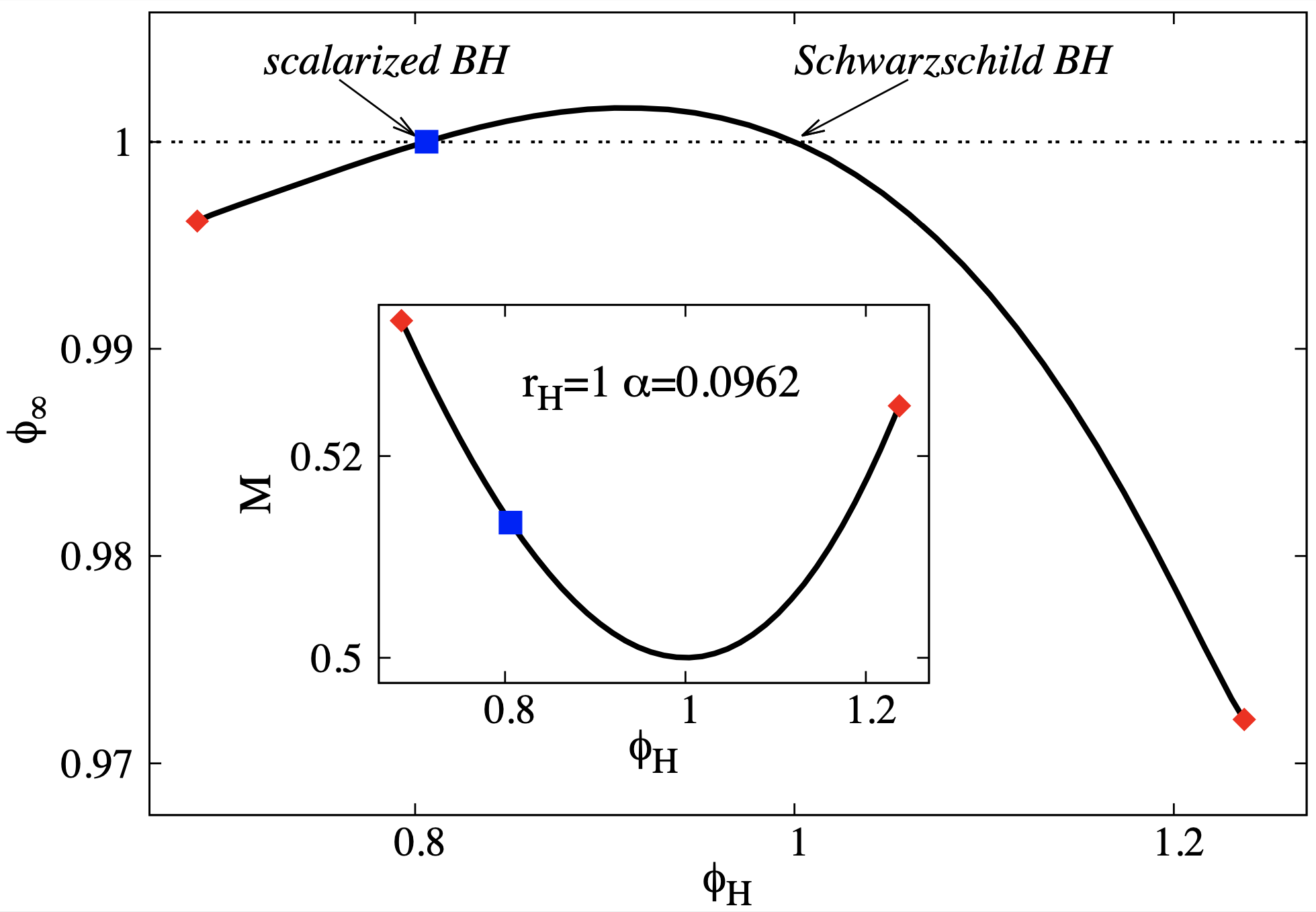
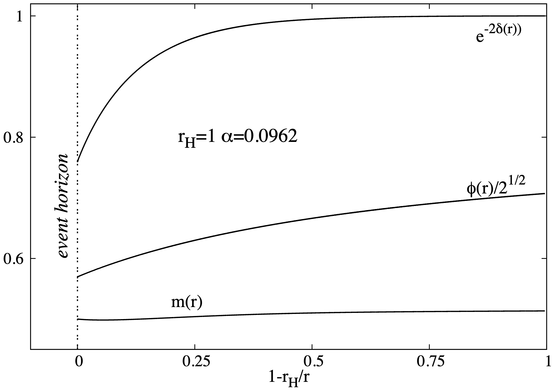
Figure 1: Left panel: The asymptotic value of the scalar field $\phi_{\infty}$ and the mass $M$ of the solutions are shown as a function of the value of the scalar field at the horizon $\phi_{H}$. The solutions have a fixed value of the horizon radius $r_{H}$ and of the coupling constant $\alpha$. Right panel: The profile of a typical scalarized solution (marked with a blue square in the left panel and Figure 2) is shown as a function of the compactified coordinate $1-r_{H}/r$.

We also display the expression of the first few terms for several quantities of interest

$$M=M^{(0)}\left(1+\frac{196}{5}\beta^{2}+\frac{8P_{1}(\phi_{0})}{3274425}\beta^{4}\right)+\dots,~{}~{}T_{H}=T_{H}^{(0)}\left(1-\frac{724}{15}\beta^{2}-\frac{8P_{2}(\phi_{0})}{3274425}\beta^{4}\right)+\dots,$$ (31)

$$S=S^{(0)}\left(1+(\frac{352}{3}-16\phi_{0})\beta^{2}+P_{3}(\phi_{0})\beta^{4}\right)+\dots,~{}~{}~{}Q_{s}=r_{H}\left(4\beta+\left(-\frac{101096}{945}-\frac{584\phi_{0}}{15}-4\phi_{0}^{2}\right)\beta^{3}\right)+\dots~{},$$

with

$$P_{1}(\phi_{0})=-418524536+693(530552-46305\phi_{0})\phi_{0},~{}~{}$$ (32)

$$P_{2}(\phi_{0})=407910422+693\phi_{0}(-1693312+113715\phi_{0}),~{}~{}$$

$$P_{3}(\phi_{0})=-\frac{143915024}{59535}+\frac{16}{225}\phi_{0}\left(31222+75(-44+\phi_{0})\phi_{0}\right)~{},$$

and

$$M^{(0)}=\frac{r_{H}}{2},~{}~{}S^{(0)}=\pi r_{H}^{2},~{}~{}T_{H}^{(0)}=\frac{1}{4\pi r_{H}}~{}.$$ (33)

One can verify that this solution provides a reasonable approximation for small $\beta$ and $\phi_{\infty}=\beta\phi_{0}$.

Of special interest, however, are the configurations with large values of $\phi_{\infty}$, which are found numerically, and may form a disconnected branch from that described by the perturbative solution above. In their construction, one starts from the expansion (18) and integrate towards $r\to\infty$ the system of three EGBs equations by using a standard ordinary differential equation solver. In practice, we integrate up to $r_{\rm max}\simeq 3\times 10^{3}r_{H}$, such that the asymptotic limit (21) is reached with enough accuracy. Given $(r_{H},~{}\phi_{\infty};~{}\alpha)$, solutions with the right asymptotics may exist for discrete set of the shooting parameters $(\phi_{H},~{}\delta_{H})$, indexed by the node number of the scalar field. Here we shall report the results for most relevant case of fundamental, nodeless solutions.

Several results in this case are displayed in Figure 1 (left panel), where we show the asymptotic value of the scalar field $\phi_{\infty}$ and mass $M$ of the solutions as a function of the scalar field value at the horizon, $\phi_{H}$. One can see that the solutions exist for a finite range of $\phi_{H}$ (located around the ground state $\phi\equiv 1$), ending in critical configurations where the condition (20) fails to be satisfied.

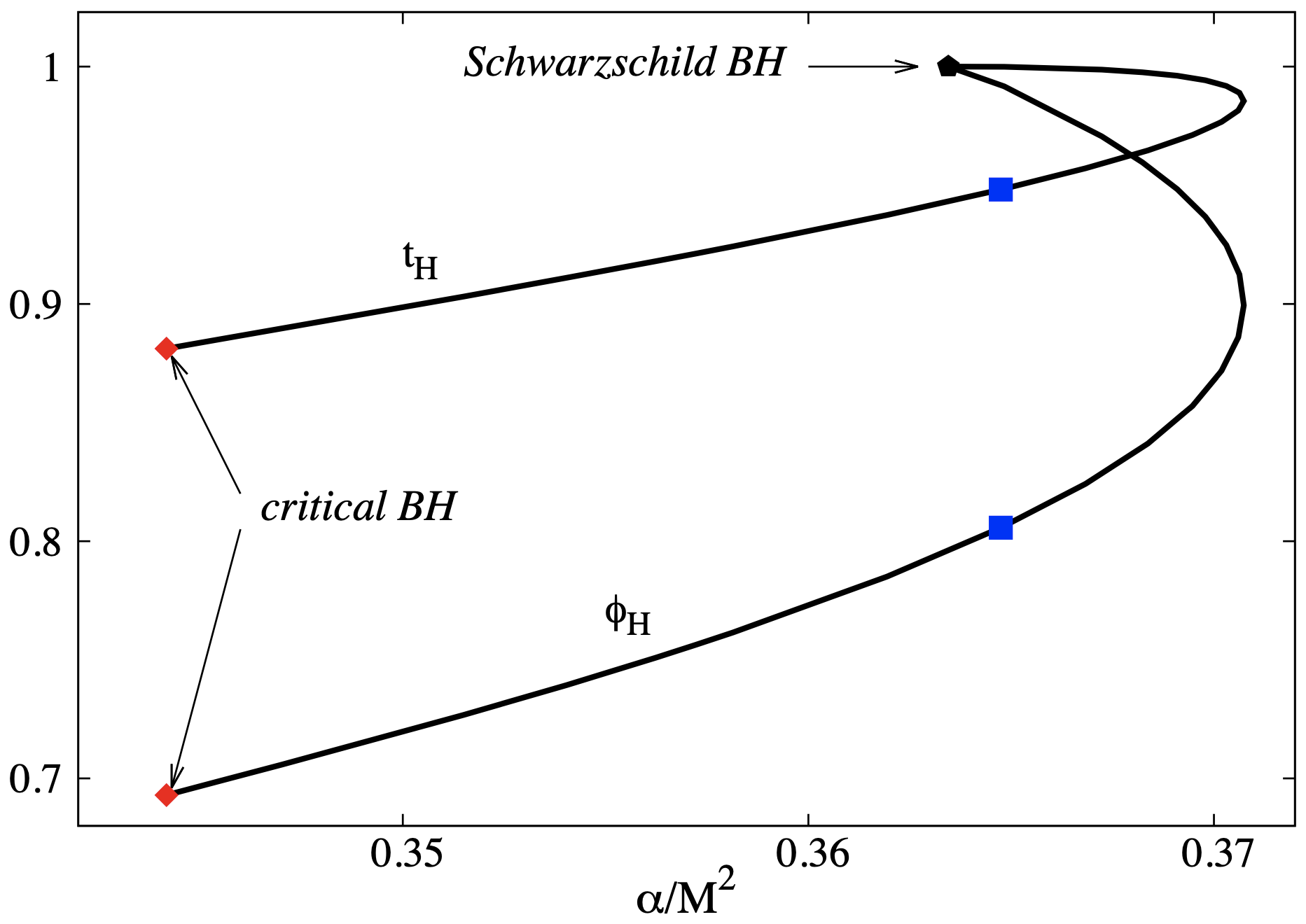
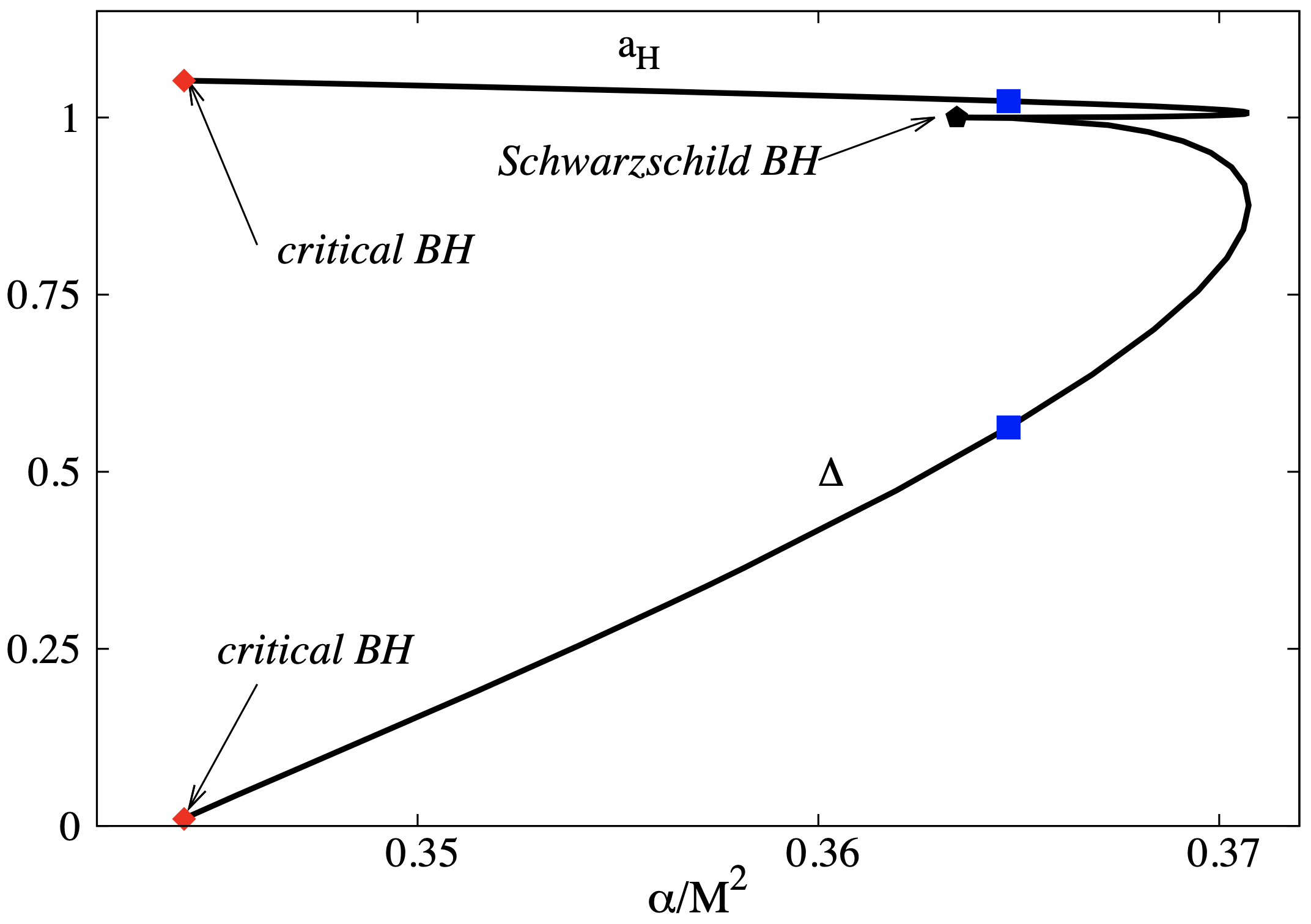
Figure 2: Several quantities of interest are shown as a function of the ratio $\alpha/M^{2}$ for the set of scalarized BHs.

3.1.2 Scalarized BHs

As one can see in Figure 1 (left panel), a particular configuration there has $\phi_{\infty}=1$, while $\phi_{H}\neq 1$. This configuration is of special interest, corresponding to a scalarized BH, its profile being displayed in Figure 1 (right panel).

That solution, however, has no special features; similar configurations are found for a range of the parameters $\alpha,r_{H}$. Also, as with the generic case, only nodeless solutions were studied so far, corresponding to the fundamental states; however, solutions with nodes exist as well, corresponding to excited EGBs configurations.

The basic properties of the scalarized BHs are rather similar to those found in [4] for a quadratic coupling function They can be summarized as follows (see Figure 2). First, these spherically symmetric BHs bifurcate from a special Schwarzschild solution supporting the scalar cloud ($i.e.$ an infinitesimally small scalar field), with $\alpha/M^{2}\simeq 0.3635$. Second, keeping constant the parameter $\alpha$ (or, equally, the event horizon radius $r_{H}$), the solutions can be obtained continuously in the parameter space, forming a line, which starts from the smooth GR Schwarzschild limit ($\phi\equiv 1$), and ends at a limiting solution. Once the limiting configuration is reached, the solutions cease to exist in the parameter space. The existence of the ‘critical’ configuration can be understood from the condition (20), with the determinant $\Delta$ vanishing at that point. Finally, as with the solutions in Ref. [4], for a given ADM mass, the entropy of the solutions is maximized by the Schwarzschild vacuum BH (although the relative difference is rather small, of order $10^{-3}$).

3.2 The scalar-vector model: perturbative solutions

The full model (15) contains also a vector field $A$, which has been consistently set to zero in the above study. The investigation of self-gravitating configurations with $A\neq 0$ is a complicated task, which we do not attempt to address here. Instead, we report the results for a preliminary investigation of scalar-vector solutions in the ‘probe limit’, $i.e.$ is for a fixed Schwarzschild BH background, as given by $\delta=0$, $N(r)=1-r_{H}/r$ in the metric Ansatz (17). This case is technically much simpler, while the corresponding solutions are likely to capture some of the basic properties of the full model.

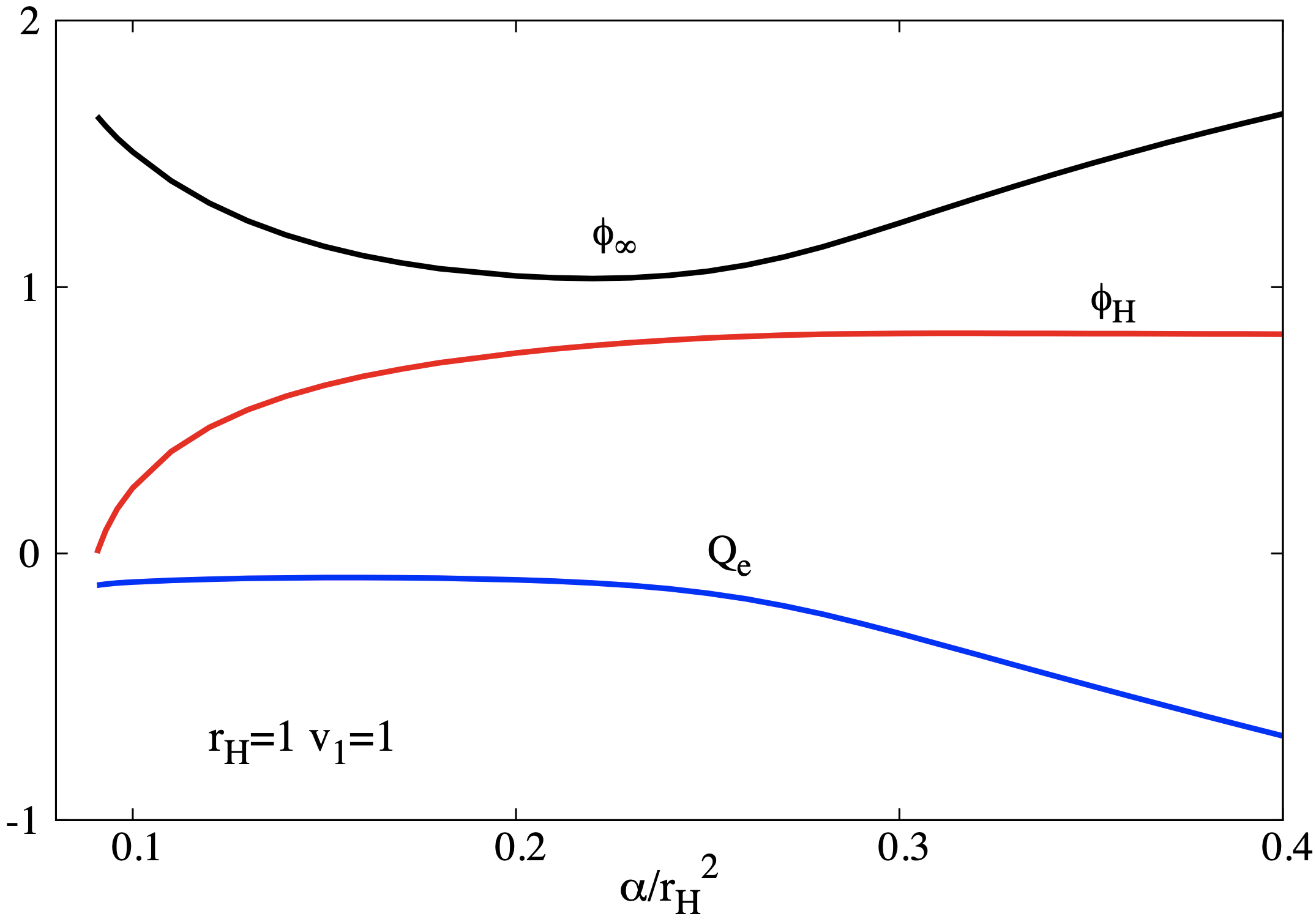
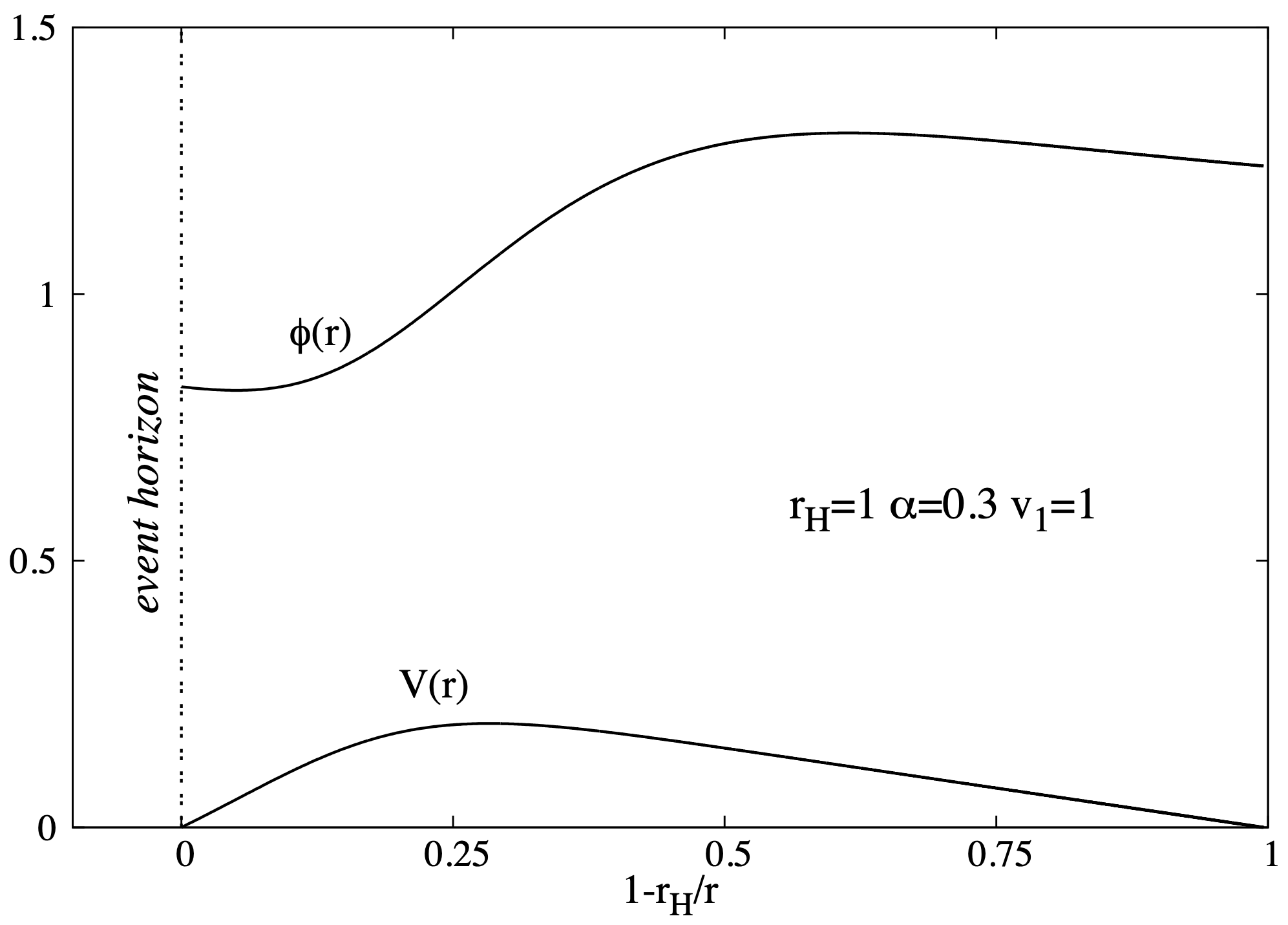
Figure 3: Left panel: The asymptotic value of the scalar field $\phi_{\infty}$, the value of the scalar field at the horizon $\phi_{H}$ and the charge of the vector field $Q_{e}$ are shown as a function of the ration $\alpha/r_{H}^{2}$ for solutions of the scalar-vector model in the probe limit. Right panel: The profile of a typical solution of the scalar-vector model in a fixed Schwarzschild BH background is shown as a function of the compactified coordinate $1-r_{H}/r$. For all solutions the vector field vanishes both at the horizon and at infinity.

Restricting again to the spherically symmetric case, we consider an ansatz with

$$\phi\equiv\phi(r),~{}~{}A=V(r)dt,$$ (34)

which can be shown to be consistent. Then, when ignoring the backreaction, the problem reduces to solving the following coupled equations

$$\phi^{\prime\prime}+\frac{2r-r_{H}}{r(r-r_{H})}\phi^{\prime}+\frac{16\alpha r_{H}^{2}}{r^{5}(r-r_{H})}\left(3(\phi^{2}-1)-\frac{r(3r-2r_{H})V^{2}}{(r-r_{H})^{2}}+\frac{2r^{2}VV^{\prime}}{(r-r_{H})}\right)=0,$$ (35)

$$V^{\prime\prime}+\frac{2V^{\prime}}{r}+\frac{32\alpha r_{H}^{2}\phi^{\prime}V}{r^{4}(r-r_{H})}=0,$$

The approximate form of the solutions close to the horizon reads

$$\phi(r)=\phi_{H}-\frac{16\alpha(r_{H}^{2}v_{1}^{2}+3(\phi_{H}^{2}-1))}{r_{H}^{3}}(r-r_{H})+O(r-r_{H})^{2},$$ (36)

$$V(r)=v_{1}(r-r_{H})-\frac{v_{1}}{r_{H}}\big{(}1-\frac{256\alpha^{2}}{r_{H}^{4}}(r_{H}^{2}v_{1}^{2}+3(\phi_{H}^{2}-1))\big{)}(r-r_{H})^{2}+O(r-r_{H})^{3},$$

where $\phi_{H}$ and $v_{1}$ are arbitrary constants. For large-$r$, the first terms in a $1/r$ expansion of the solution reads

$$\phi(r)=\phi_{\infty}+\frac{Q_{s}}{r}+O(1/r^{2}),~{}~{}V(r)=V_{\infty}+\frac{Q_{e}}{r}+O(1/r^{5}),$$ (37)

with $\phi_{\infty}$, $V_{\infty}$, $Q_{e}$ and $Q_{s}$ free parameters.

Eqs. (35) are solved numerically, by using the same approach as in the EGBs case. The numerical results indicate the existence, for any $\alpha$, of a continuum of solutions in terms of the constants $\phi_{H}$, $v_{1}$ which enter the near horizon expansion (36). The asymptotic values of the scalar and vector fields depend of the input parameters $\phi_{H}$, $v_{1}$, $r_{H}$ and $\alpha$ (note that, as expected from the structure of the equations, the vector field vanishes identically, when taking $v_{1}=0$).

Of special interest here are the configurations which approach asymptotically the vector ground state, $i.e.$ with $V_{\infty}=0$. In Figure 3 (left panel) we display some quantities of interest for a set of such solutions; there the values of $r_{H}$ and $v_{1}$ are fixed, while the parameter $\alpha$ is varied (note that we restrict again to the case of nodeless configurations). One can notice that, for a given $\alpha$, the solution with $V(\infty)=0$ is found for a single value of $\phi_{H}$ while $\phi_{\infty}\neq 1$. The profile of a typical solution is shown in Figure 3 (right panel).

The presence of probe-limit solutions with $V_{\infty}=0$ provides a hint for the existence of vectorized configurations in the full backreacting model. That is, the generic solutions above with $\phi_{\infty}\neq 1$ may possess generalizations with a nonzero vector field in the bulk, and still approach asymptotically the vector ground state. We hope to return to the study of these configurations elsewhere.

4 Further remarks

The main purpose of this work was to point out that families of EGBs models with coupling functions that permit spontaneous scalarization can be motivated by a geometric/topological construction [41, 42]. This indicates a more natural embedding for GB spontaneous scalarization models; typically the necessary coupling is simply postulated ad hoc. Moreover, as a case study, we present a preliminary investigation of the scalarized BH solutions in a particular EGBs model emerging from this sort of construction.

The models discussed herein offer both novel features and challenges. As for the novel features, the corresponding coupling function is a sum of a linear and a cubic term, with the scalar field possessing two disconnected ground states. A consequence of this fact is that the BH scalarization becomes possible for any sign of the coupling constant $\alpha$ in front of the GB term (but around a different vacuum for each sign). As for the challenges, the cubic term (or, in general, the highest odd power term) raises the issue of the stability of the model. Moroever, the construction is not complete: it provides the GB term and the non-minimal couplings, but the resulting HCSG term has been added ad hoc to the standard Einstein-scalar field action.

The basic properties of the scalarized BHs constructed herein were found to be rather similar to those in the original work [4], where a quadratic coupling function has been employed. In particular, the scalarized BHs are entropically disfavoured over the Schwarzschild vacuum configuration. Generic solutions (with a scalar field which does not approach asymptotically the ground state) were also studied, and a perturbative solution was reported.

A preliminary investigation of the solutions of the general model in [41] with an extra-vector field has been also considered. Only the probe limit regime of the solutions ($i.e.$ for a fixed Schwarzschild background) has been considered in this case, the results hinting towards the possible existence of ’vectorized’ BHs within the full model.

Acknowledgements
The work of E.R. is supported by the Center for Research and Development in Mathematics and Applications (CIDMA) through the Portuguese Foundation for Science and Technology (FCT - Fundacao para a Ciência e a Tecnologia), references UIDB/04106/2020 and UIDP/04106/2020, and by national funds (OE), through FCT, I.P., in the scope of the framework contract foreseen in the numbers 4, 5 and 6 of the article 23,of the Decree-Law 57/2016, of August 29, changed by Law 57/2017, of July 19. We acknowledge support from the projects PTDC/FIS-OUT/28407/2017, CERN/FIS-PAR/0027/2019 and PTDC/FIS-AST/3041/2020. This work has further been supported by the European Union’s Horizon 2020 research and innovation (RISE) programme H2020-MSCA-RISE-2017 Grant No. FunFiCO-777740. The authors would like to acknowledge networking support by the COST Action CA16104.

References

- [1] C. A. R. Herdeiro and E. Radu, Int. J. Mod. Phys. D 24 (2015) no.09, 1542014 [arXiv:1504.08209 [gr-qc]].
- [2] D. Astefanesei, C. Herdeiro, J. Oliveira and E. Radu, JHEP 09 (2020), 186 [arXiv:2007.04153 [gr-qc]].
- [3] J. L. Blázquez-Salcedo, C. A. R. Herdeiro, J. Kunz, A. M. Pombo and E. Radu, Phys. Lett. B 806 (2020), 135493 [arXiv:2002.00963 [gr-qc]].
- [4] H. O. Silva, J. Sakstein, L. Gualtieri, T. P. Sotiriou and E. Berti, Phys. Rev. Lett. 120 (2018) no.13, 131104 [arXiv:1711.02080 [gr-qc]].
- [5] D. D. Doneva and S. S. Yazadjiev, Phys. Rev. Lett. 120 (2018) no.13, 131103 [arXiv:1711.01187 [gr-qc]].
- [6] G. Antoniou, A. Bakopoulos and P. Kanti, Phys. Rev. Lett. 120 (2018) no.13, 131102 [arXiv:1711.03390 [hep-th]].
- [7] G. Antoniou, A. Bakopoulos and P. Kanti, Phys. Rev. D 97 (2018) no.8, 084037 [arXiv:1711.07431 [hep-th]].
- [8] M. Minamitsuji and T. Ikeda, Phys. Rev. D 99 (2019) no.4, 044017 [arXiv:1812.03551 [gr-qc]].
- [9] Y. Brihaye and L. Ducobu, Phys. Lett. B 795 (2019), 135-143 [arXiv:1812.07438 [gr-qc]].
- [10] C. F. B. Macedo, J. Sakstein, E. Berti, L. Gualtieri, H. O. Silva and T. P. Sotiriou, Phys. Rev. D 99 (2019) no.10, 104041 [arXiv:1903.06784 [gr-qc]].
- [11] D. D. Doneva, K. V. Staykov and S. S. Yazadjiev, Phys. Rev. D 99 (2019) no.10, 104045 [arXiv:1903.08119 [gr-qc]].
- [12] N. Andreou, N. Franchini, G. Ventagli and T. P. Sotiriou, Phys. Rev. D 99 (2019) no.12, 124022 [erratum: Phys. Rev. D 101 (2020) no.10, 109903] [arXiv:1904.06365 [gr-qc]].
- [13] M. Minamitsuji and T. Ikeda, Phys. Rev. D 99 (2019) no.10, 104069 [arXiv:1904.06572 [gr-qc]].
- [14] J. L. Blázquez-Salcedo, S. Kahlen and J. Kunz, Symmetry 12 (2020) no.12, 2057 [arXiv:2011.01326 [gr-qc]].
- [15] H. Guo, X. M. Kuang, E. Papantonopoulos and B. Wang, [arXiv:2012.11844 [gr-qc]].
- [16] A. Bakopoulos, P. Kanti and N. Pappas, Phys. Rev. D 101 (2020) no.8, 084059 [arXiv:2003.02473 [hep-th]].
- [17] Y. Peng, Phys. Lett. B 807 (2020), 135569 [arXiv:2004.12566 [gr-qc]].
- [18] H. S. Liu, H. Lu, Z. Y. Tang and B. Wang, [arXiv:2004.14395 [gr-qc]].
- [19] V. Cardoso, A. Foschi and M. Zilhao, Phys. Rev. Lett. 124 (2020) no.22, 221104 [arXiv:2005.12284 [gr-qc]].
- [20] G. Ventagli, A. Lehébel and T. P. Sotiriou, Phys. Rev. D 102 (2020) no.2, 024050 [arXiv:2006.01153 [gr-qc]].
- [21] H. Guo, S. Kiorpelidi, X. M. Kuang, E. Papantonopoulos, B. Wang and J. P. Wu, Phys. Rev. D 102 (2020) no.8, 084029 [arXiv:2006.10659 [hep-th]].
- [22] D. D. Doneva, K. V. Staykov, S. S. Yazadjiev and R. Z. Zheleva, Phys. Rev. D 102 (2020) no.6, 064042 [arXiv:2006.11515 [gr-qc]].
- [23] M. Heydari-Fard and H. R. Sepangi, [arXiv:2009.13748 [gr-qc]].
- [24] A. Bakopoulos, [arXiv:2010.13189 [gr-qc]].
- [25] J. L. Blázquez-Salcedo, D. D. Doneva, J. Kunz and S. S. Yazadjiev, Phys. Rev. D 98 (2018) no.8, 084011 [arXiv:1805.05755 [gr-qc]].
- [26] H. O. Silva, C. F. B. Macedo, T. P. Sotiriou, L. Gualtieri, J. Sakstein and E. Berti, Phys. Rev. D 99 (2019) no.6, 064011 [arXiv:1812.05590 [gr-qc]].
- [27] J. L. Blázquez-Salcedo, D. D. Doneva, S. Kahlen, J. Kunz, P. Nedkova and S. S. Yazadjiev, Phys. Rev. D 101 (2020) no.10, 104006 [arXiv:2003.02862 [gr-qc]].
- [28] J. L. Blázquez-Salcedo, D. D. Doneva, S. Kahlen, J. Kunz, P. Nedkova and S. S. Yazadjiev, Phys. Rev. D 102 (2020) no.2, 024086 [arXiv:2006.06006 [gr-qc]].
- [29] S. Hod, Phys. Rev. D 100 (2019) no.6, 064039 [arXiv:1912.07630 [gr-qc]].
- [30] S. Hod, Eur. Phys. J. C 79 (2019) no.11, 966 [arXiv:2101.02219 [gr-qc]].
- [31] R. A. Konoplya and A. Zhidenko, Phys. Rev. D 100 (2019) no.4, 044015 [arXiv:1907.05551 [gr-qc]].
- [32] S. Hod, Phys. Rev. D 102 (2020) no.8, 084060 [arXiv:2006.09399 [gr-qc]].
- [33] P. V. P. Cunha, C. A. R. Herdeiro and E. Radu, Phys. Rev. Lett. 123 (2019) no.1, 011101 [arXiv:1904.09997 [gr-qc]].
- [34] L. G. Collodel, B. Kleihaus, J. Kunz and E. Berti, Class. Quant. Grav. 37 (2020) no.7, 075018 [arXiv:1912.05382 [gr-qc]].
- [35] D. D. Doneva and S. S. Yazadjiev, [arXiv:2101.03514 [gr-qc]].
- [36] A. Dima, E. Barausse, N. Franchini and T. P. Sotiriou, Phys. Rev. Lett. 125 (2020) no.23, 231101 [arXiv:2006.03095 [gr-qc]].
- [37] C. A. R. Herdeiro, E. Radu, H. O. Silva, T. P. Sotiriou and N. Yunes, Phys. Rev. Lett. 126 (2021) no.1, 011103 [arXiv:2009.03904 [gr-qc]].
- [38] E. Berti, L. G. Collodel, B. Kleihaus and J. Kunz, Phys. Rev. Lett. 126 (2021) no.1, 011104 [arXiv:2009.03905 [gr-qc]].
- [39] D. D. Doneva, L. G. Collodel, C. J. Krüger and S. S. Yazadjiev, Phys. Rev. D 102 (2020) no.10, 104027 [arXiv:2008.07391 [gr-qc]].
- [40] A. Buonanno, M. Gasperini and C. Ungarelli, Mod. Phys. Lett. A 12, 1883-1889 (1997) [arXiv:hep-th/9707053 [hep-th]].
- [41] D. H. Tchrakian, Phys. Atom. Nucl. 81 (2018) no.6, 930 [arXiv:1712.05190 [gr-qc]].
- [42] E. Radu and D. H. Tchrakian, Phys. Part. Nucl. Lett. 17 (2020) no.5, 753-759.
- [43] R. Utiyama, Phys. Rev. 101 (1956), 1597-1607
- [44] T. W. B. Kibble, J. Math. Phys. 2 (1961), 212-221
- [45] E. Witten, Nucl. Phys. B 311 (1988) 46.
- [46] A. H. Chamseddine, Phys. Lett. B 233 (1989) 291.
- [47] A. H. Chamseddine, Nucl. Phys. B 346 (1990) 213.
- [48] S. Deser, R. Jackiw and S. Templeton, Annals Phys. 140 (1982) 372 [Annals Phys. 185 (1988) 406] [Annals Phys. 281 (2000) 409].
- [49] T. Tchrakian, J. Phys. A 44 (2011) 343001 [arXiv:1009.3790 [hep-th]].
- [50] E. Radu and T. Tchrakian, arXiv:1101.5068 [hep-th].
- [51] D. H. Tchrakian, J. Phys. A 48 (2015) no.37, 375401 [arXiv:1505.05344 [hep-th]].
- [52] D. H. Tchrakian, Int. J. Mod. Phys. A 35 (2020) no.05, 2050022 [arXiv:1910.00315 [gr-qc]].
- [53] J. F. M. Delgado, C. A. R. Herdeiro and E. Radu, JHEP 04 (2020), 180 [arXiv:2002.05012 [gr-qc]].
- [54] T. P. Sotiriou and S. Y. Zhou, Phys. Rev. Lett. 112 (2014) 251102 [arXiv:1312.3622 [gr-qc]].
- [55] T. P. Sotiriou and S. Y. Zhou, Phys. Rev. D 90 (2014) 124063 [arXiv:1408.1698 [gr-qc]].
- [56] G. W. Horndeski, Int. J. Theor. Phys. 10 (1974) 363.
- [57] R. M. Wald, Phys. Rev. D 48 (1993) 3427 [arXiv:gr-qc/9307038].
- [58] S. Barton, B. Hartmann, B. Kleihaus and J. Kunz, [arXiv:2103.01651 [gr-qc]].