Hypercorrelation Squeeze for Few-Shot Segmentation

Abstract

Few-shot semantic segmentation aims at learning to segment a target object from a query image using only a few annotated support images of the target class. This challenging task requires to understand diverse levels of visual cues and analyze fine-grained correspondence relations between the query and the support images. To address the problem, we propose Hypercorrelation Squeeze Networks (HSNet) that leverages multi-level feature correlation and efficient 4D convolutions. It extracts diverse features from different levels of intermediate convolutional layers and constructs a collection of 4D correlation tensors, i.e., hypercorrelations. Using efficient center-pivot 4D convolutions in a pyramidal architecture, the method gradually squeezes high-level semantic and low-level geometric cues of the hypercorrelation into precise segmentation masks in coarse-to-fine manner. The significant performance improvements on standard few-shot segmentation benchmarks of PASCAL-5ⁱ, COCO-20ⁱ, and FSS-1000 verify the efficacy of the proposed method.

1 Introduction

The advent of deep convolutional neural networks [17, 20, 64] has promoted dramatic advances in many computer vision tasks including object tracking [28, 29, 45], visual correspondence [22, 44, 48], and semantic segmentation [7, 47, 62] to name a few. Despite the effectiveness of deep networks, their demand for a heavy amount of annotated examples from large-scale datasets [9, 11, 35] still remains a fundamental limitation since data labeling requires substantial human efforts, especially for dense prediction tasks, e.g., semantic segmentation. To cope with the challenge, there have been various attempts in semi- and weakly-supervised segmentation approaches [6, 26, 39, 66, 72, 77, 88] which in turn effectively alleviated the data-hunger issue. However, given only a few annotated training examples, the problem of poor generalization ability of the deep networks is yet the primary concern that many few-shot segmentation methods [10, 12, 13, 19, 33, 36, 37, 46, 54, 61, 63, 69, 70, 74, 75, 80, 83, 86, 87, 89] struggle to address.

Figure 1: Our model performs visual reasoning in coarse-to-fine manner by gradually squeezing high-dimensional hypercorrelation to the target segmentation mask with efficient 4D convolutions.

In contrast, human visual system easily achieves generalizing appearances of new objects given extremely limited supervision. The crux of such intelligence lies at the ability in finding reliable correspondences across different instances of the same class. Recent work on semantic correspondence shows that leveraging dense intermediate features [38, 42, 44] and processing correlation tensors with high-dimensional convolutions [30, 58, 71] are significantly effective in establishing accurate correspondences. However, while recent few-shot segmentation research began active exploration in the direction of correlation learning, most of them [36, 37, 46, 65, 73, 75, 80] neither exploit diverse levels of feature representations from early to late layers of a CNN nor construct pair-wise feature correlations to capture fine-grained correlation patterns. There have been some attempts [74, 86] in utilizing dense correlations with multi-level features, but they are yet limited in the sense that they simply employ the dense correlations for graph attention, using only a small fraction of intermediate conv layers.

In this work we combine the two of the most influential techniques in recent research of visual correspondence, multi-level features and 4D convolutions, and deign a novel framework, dubbed Hypercorrelation Squeeze Networks (HSNet), for the task of few-shot semantic segmentation. As illustrated in Fig. 1, our network exploits diverse geometric/semantic feature representations from many different intermediate CNN layers to construct a collection of 4D correlation tensors, i.e., hypercorrelations, which represent a rich set of correspondences in multiple visual aspects. Following the work of FPN [34], we adapt pyramidal design to capture both high-level semantic and low-level geometric cues for precise mask prediction in coarse-to-fine manner using deeply stacked 4D conv layers. To reduce computational burden caused by such heavy use of high-dimensional convs, we devise an efficient 4D kernel via reasonable weight-sparsification which enables real-time inference while being more effective and light-weight than the existing ones. The improvements on standard few-shot segmentation benchmarks of PASCAL-5ⁱ [61], COCO-20ⁱ [35], and FSS-1000 [33] verify the efficacy of the proposed method.

2 Related Work

Semantic segmentation. The goal of semantic segmentation is to classify each pixel of an image into one of the predefined object categories. Prevalent segmentation approaches [5, 7, 47, 49, 52, 62, 76] typically employ encoder-decoder structure in their architecture; the encoder aggregates features along deep convolutional pathways and provides high-dimensional feature map in low-resolution and the corresponding decoder takes the output to predict segmentation mask by reversing this process [49]. Although the methods clearly show the effectiveness of the encoder-decoder architecture in the task of semantic segmentation, offering useful insights to our study, they still suffer apparent disadvantages of data-driven nature of neural networks: lack of generalizibility under insufficient training data.

Few-shot learning. To resolve the generalization problem, many recent approaches to image classification made various attempts in training deep networks with a few annotated examples [1, 18, 25, 31, 50, 53, 59, 65, 67, 73, 79, 84, 85]. Vinyals et al. [73] propose matching networks for one-shot learning; the method utilizes a special kind of mini-batches called episodes to match training and testing environments, facilitating better generalization on novel classes. Snell et al. [65] introduce prototypical networks which compute distances between representative embeddings, i.e., prototypes, for few-shot classification. With the growing interests in few-shot learning in classification domain, the problem of few-shot segmentation has attracted a great deal of attention as well. Shaban et al. [61] propose one-shot semantic segmentation networks which (meta-) learns to generate parameters of FCN [62]. Inspired by the prototypical networks [65], utilizing prototype representations to guide mask prediction in a query image became a popular paradigm in few-shot segmentation literature [10, 36, 37, 46, 63, 75, 80, 87, 89]. Witnessing the limitation of prototypical approaches, e.g., loss of spatial structure due to masked average pooling [89], work of [74, 86] build pair-wise feature correlations, e.g., graph attention, to retain the spatial structure of the images for fine-grained mask prediction. Note that both prototypical and graph-based methods fundamentally focus on learning to find reliable correspondences between support and query images for accurate mask prediction. In this work, we advance this idea and focus on learning to analyze correspondences using adequately designed learnable layers, e.g., 4D convolutions [58], for effective semantic segmentation.

Learning visual correspondences. The task of visual correspondence aims to find reliable correspondences under challenging degree of variations [3, 14, 15, 43, 60]. Many methods [21, 22, 30, 38, 42, 44, 56, 58, 81] typically built upon convolutional features pretrained on classification task [9], showing they serve as good transferable representations. Recent approaches to semantic correspondence [21, 38, 42, 44] show that efficiently exploiting different levels of convolutional features distributed over all intermediate layers clearly benefits matching accuracy. In wide-baseline matching literature, a trending choice is to employ 4D convolutions [30, 41, 57, 58, 71] on dense feature matches to identify spatially consistent matches by analyzing local patterns in 4D space. The use of multi-level features and relational pattern analysis using 4D convs are the two widely adopted techniques in the field of visual correspondence.

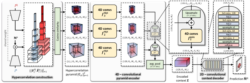
Figure 2: Overall architecture of the proposed network which consists of three main parts: hypercorrelation construction, 4D-convolutional pyramid encoder, and 2D-convolutional context decoder. We refer the readers to Sec. 4 for details of the architecture.

In this paper we adapt the two most influential methodologies in visual correspondence to tackle few-shot segmentation: multi-level features and 4D convolutions. Inspired by the previous matching methods [42, 44, 27], which use multi-level features to build effective “appearance features”, we construct high-dimensional “relational features” using intermediate CNN features and process them with a series of 4D convolutions. However, their quadratic complexity still remains a major bottleneck in designing cost-effective deep networks, constraining many previous matching methods [30, 57, 58, 71] to use only a few 4D conv layers. To resolve the issue, we develop a light-weight 4D convolutional kernel by collecting only a small subset of vital parameters for effective pattern recognition, which eventually leads to an efficient decomposition into a pair of 2D conv kernels with a linear complexity. Our contributions can be summarized as follows:

• We present the Hypercorrelation Squeeze Networks that analyze dense feature matches of diverse visual aspects using deeply stacked 4D conv layers.

• We propose center-pivot 4D conv kernel which is more effective than the existing one in terms both accuracy and speed, achieving real-time inference.

• The proposed method sets a new state of the art on three standard few-shot segmentation benchmarks: PASCAL-5ⁱ [61], COCO-20ⁱ [35], and FSS-1000 [33].

3 Problem Setup

The goal of few-shot semantic segmentation is to perform segmentation given only a few annotated examples. To avoid the risk of overfitting due to insufficient training data, we adopt widely used meta-learning approach called episodic training [73]. Let us denote respective training and test sets as $\mathcal{D}_{\text{train}}$ and $\mathcal{D}_{\text{test}}$ which are disjoint with respect to object classes. Both sets consist of multiple episodes each of which is composed of a support set $\mathcal{S}=({I}^{\mathrm{s}},\mathbf{M}^{\mathrm{s}})$ and a query set $\mathcal{Q}=({I}^{\mathrm{q}},\mathbf{M}^{\mathrm{q}})$ where ${I}^{*}$ and $\mathbf{M}^{*}$ are an image and its corresponding mask label respectively. During training, our model iteratively samples an episode from $\mathcal{D}_{\text{train}}$ to learn a mapping from $({I}^{\mathrm{s}},\mathbf{M}^{\mathrm{s}},{I}^{\mathrm{q}})$ to query mask $\mathbf{M}^{\mathrm{q}}$. Once the model is trained, it uses the learned mapping for evaluation without further optimization, i.e., the model takes randomly sampled $({I}^{\mathrm{s}},\mathbf{M}^{\mathrm{s}},{I}^{\mathrm{q}})$ from $\mathcal{D}_{\text{test}}$ to predict query mask.

4 Proposed Approach

In this section, we present a novel few-shot segmentation architecture, Hypercorrelation Squeeze Networks (HSNet), which capture relevant patterns in multi-level feature correlations between a pair of input images to predict fine-grained segmentation mask in a query image. As illustrated in Fig. 2, we adopt an encoder-decoder structure in our architecture; the encoder gradually squeezes dimension of the input hypercorrelations by aggregating their local information to a global context, and the decoder processes the encoded context to predict a query mask. In Sec. 4.1-4.3, we demonstrate each pipeline in one-shot setting, i.e., the model predicts the query mask given ${I}^{\mathrm{q}}$ and $\mathcal{S}=({I}^{\mathrm{s}},\mathbf{M}^{\mathrm{s}})$. In Sec. 4.4, to mitigate large resource demands of 4D convs, we present a light-weight 4D kernel which greatly improves model efficiency in terms of both memory and time. In Sec. 4.5, we demonstrate how the model can be easily extended to $K$-shot setting, i.e., $\mathcal{S}=\{({I}^{\mathrm{s}}_{k},\mathbf{M}^{\mathrm{s}}_{k})\}_{k=1}^{K}$, without loss of generality.

4.1 Hypercorrelation construction

Inspired by recent semantic matching approaches [38, 42, 44], our model exploits a rich set of features from the intermediate layers of a convolutional neural network to capture multi-level semantic and geometric patterns of similarities between the support and query images. Given a pair of query and support images, ${I}^{\mathrm{q}},{I}^{\mathrm{s}}\in\mathbb{R}^{3\times H\times W}$, the backbone network produces a sequence of $L$ pairs of intermediate feature maps $\{(\mathbf{F}^{\mathrm{q}}_{l},\mathbf{F}^{\mathrm{s}}_{l})\}_{l=1}^{L}$. We mask each support feature map $\mathbf{F}^{\mathrm{s}}_{l}\in\mathbb{R}^{C_{l}\times H_{l}\times W_{l}}$ using the support mask $\mathbf{M}^{\mathrm{s}}\in\{0,1\}^{H\times W}$ to discard irrelevant activations for reliable mask prediction:

$$\hat{\mathbf{F}}^{\mathrm{s}}_{l}=\mathbf{F}^{\mathrm{s}}_{l}\odot\zeta_{l}(\mathbf{M}^{\mathrm{s}}),$$ (1)

where $\odot$ is Hadamard product and $\zeta_{l}(\cdot)$ is a function that bilinearly interpolates input tensor to the spatial size of the feature map $\mathbf{F}^{\mathrm{s}}_{l}$ at layer $l$ followed by expansion along channel dimension such that $\zeta_{l}:\mathbb{R}^{H\times W}\xrightarrow{}\mathbb{R}^{C_{l}\times H_{l}\times W_{l}}$. For the subsequent hypercorrleation construction, a pair of query and masked support features at each layer forms a 4D correlation tensor $\mathbf{\hat{C}}_{l}\in\mathbb{R}^{H_{l}\times W_{l}\times H_{l}\times W_{l}}$ using cosine similarity:

$$\mathbf{\hat{C}}_{l}(\mathbf{x}^{\mathrm{q}},\mathbf{x}^{\mathrm{s}})=\text{ReLU}\Bigg{(}\frac{\mathbf{F}^{\mathrm{q}}_{l}(\mathbf{x}^{\mathrm{q}})\cdot\hat{\mathbf{F}}^{\mathrm{s}}_{l}(\mathbf{x}^{\mathrm{s}})}{\lVert\mathbf{F}^{\mathrm{q}}_{l}(\mathbf{x}^{\mathrm{q}})\rVert\lVert\hat{\mathbf{F}}^{\mathrm{s}}_{l}(\mathbf{x}^{\mathrm{s}})\rVert}\Bigg{)},$$ (2)

where $\mathbf{x}^{\mathrm{q}}$ and $\mathbf{x}^{\mathrm{s}}$ denote 2-dimensional spatial positions of feature maps $\mathbf{F}^{\mathrm{q}}_{l}$ and $\hat{\mathbf{F}}^{\mathrm{s}}_{l}$ respectively, and ReLU suppresses noisy correlation scores. From the resultant set of 4D correlations $\{\mathbf{\hat{C}}_{l}\}_{l=1}^{L}$, we collect 4D tensors if they have the same spatial sizes and denote the subset as $\{\mathbf{\hat{C}}_{l}\}_{l\in\mathcal{L}_{p}}$ where $\mathcal{L}_{p}$ is a subset of CNN layer indices $\{1,...,L\}$ at some pyramidal layer $p$. Finally, all the 4D tensors in $\{\mathbf{\hat{C}}_{l}\}_{l\in\mathcal{L}_{p}}$ are concatenated along channel dimension to form a hypercorrelation $\mathbf{C}_{p}\in\mathbb{R}^{|\mathcal{L}_{p}|\times H_{p}\times W_{p}\times H_{p}\times W_{p}}$ where $(H_{p},W_{p},H_{p},W_{p})$, with abuse of notation, represents the spatial resolution of the hypercorrelation at pyramidal layer $p$. Given $P$ pyramidal layers, we denote hypercorrelation pyramid as $\mathcal{C}=\{\mathbf{C}_{p}\}_{p=1}^{P}$, representing a rich collection of feature correlations from multiple visual aspects.

4.2 4D-convolutional pyramid encoder

Our encoder network takes the hypercorrelation pyramid $\mathcal{C}=\{\mathbf{C}_{p}\}_{p=1}^{P}$ to effectively squeeze it into a condensed feature map $\mathbf{Z}\in\mathbb{R}^{128\times H_{1}\times W_{1}}$. We achieve this correlation learning using two types of building blocks: a squeezing block $f_{p}^{\text{sqz}}$ and a mixing block $f_{p}^{\text{mix}}$. Each block consists of three sequences of multi-channel 4D convolution, group normalization [78], and ReLU activation as illustrated in Fig. 3. In the squeezing block $f_{p}^{\text{sqz}}$, large strides periodically squeeze the last two (support) spatial dimensions of $\mathbf{C}_{p}$ down to $(H_{\epsilon},W_{\epsilon})$ while the first two spatial (query) dimensions remain the same as $(H_{p},W_{p})$, i.e., $f^{\text{sqz}}_{p}:\mathbb{R}^{|\mathcal{L}_{p}|\times H_{p}\times W_{p}\times H_{p}\times W_{p}}\xrightarrow{}\mathbb{R}^{128\times H_{p}\times W_{p}\times H_{\epsilon}\times W_{\epsilon}}$ where $H_{p}>H_{\epsilon}$ and $W_{p}>W_{\epsilon}$. Similar to FPN [34] structure, two outputs from adjacent pyramidal layers, $p$ and $p+1$, are merged by element-wise addition after upsampling the (query) spatial dimensions of the upper layer output by a factor of 2. The mixing block $f^{\text{mix}}_{p}:\mathbb{R}^{128\times H_{p}\times W_{p}\times H_{\epsilon}\times W_{\epsilon}}\xrightarrow{}\mathbb{R}^{128\times H_{p}\times W_{p}\times H_{\epsilon}\times W_{\epsilon}}$ then processes this mixture with 4D convolutions to propagate relevant information to lower layers in a top-down fashion. After the iterative propagation, the output tensor of the lowest mixing block $f_{1}^{\text{mix}}$ is further compressed by average-pooling its last two (support) spatial dimensions, which in turn provides a 2-dimensional feature map $\mathbf{Z}\in\mathbb{R}^{128\times H_{1}\times W_{1}}$ that signifies a condensed representation of the hypercorrelation $\mathcal{C}$.

4.3 2D-convolutional context decoder

The decoder network consists of a series of 2D convolutions, ReLU, and upsampling layers followed by softmax function as illustrated in Fig. 2. The network takes the context representation $\mathbf{Z}$ and predicts two-channel map $\mathbf{\hat{M}}^{\mathrm{q}}\in[0,1]^{2\times H\times W}$ where two channel values indicate probabilities of foreground and background. During training, the network parameters are optimized using the mean of cross-entropy loss between the prediction $\mathbf{\hat{M}}^{\mathrm{q}}$ and the ground-truth $\mathbf{M}^{\mathrm{q}}$ over all pixel locations. During testing, we take the maximum channel value at each pixel to obtain final query mask prediction $\mathbf{\bar{M}}^{\mathrm{q}}\in\{0,1\}^{H\times W}$ for evaluation.

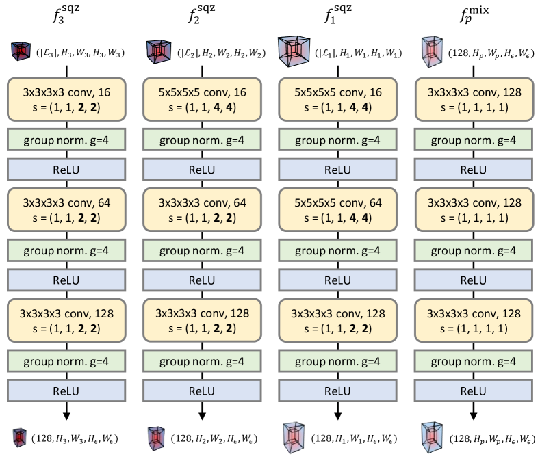
Figure 3: Building blocks in Hypercorrelation Squeeze Networks. $s$ and $g$ denotes strides of 4D conv and the number of groups in group normalization [78] respectively. Note $p\in\{1,2\}$ for $f_{p}^{\text{mix}}$.

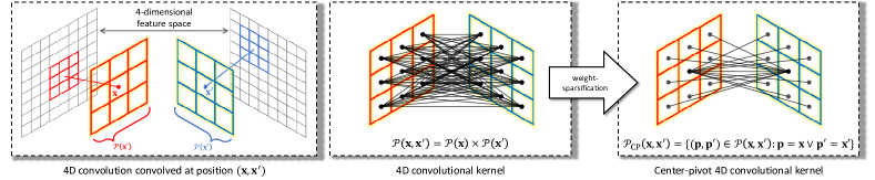
Figure 4: 4D convolution (left) and weights of 4D kernel [58, 81] (middle) and center-pivot 4D kernel (right). Each black wire that connects two different pixel locations represents a single weight of the 4D kernel. The kernel size used in this example is $(3,3,3,3)$, i.e., $\hat{k}=3$.

4.4 Center-pivot 4D convolution

Apparently, our network with such a large number of 4D convolutions demands a substantial amount of resources due to the curse of dimensionality, which constrained many visual correspondence methods [22, 30, 32, 58, 71] to use only a few 4D conv layers. To address the concern, we revisit the 4D convolution operation and delve into its limitations. Then we demonstrate how a unique weight-sparsification scheme effectively resolves the issues.

4D convolution and its limitation. Typical 4D convolution parameterized by a kernel ${k}\in\mathbb{R}^{\hat{k}\times\hat{k}\times\hat{k}\times\hat{k}}$ on a correlation tensor $c\in\mathbb{R}^{H\times W\times H\times W}$ at position $(\mathbf{x},\mathbf{x}^{\prime})\in\mathbb{R}^{4}$ is formulated as

$$({c}*{k})(\mathbf{x},\mathbf{x}^{\prime}) =\sum_{(\mathbf{p},\mathbf{p}^{\prime})\in\mathcal{P}(\mathbf{x},\mathbf{x}^{\prime})}{c}(\mathbf{p},\mathbf{p}^{\prime}){k}(\mathbf{p}-\mathbf{x},\mathbf{p}^{\prime}-\mathbf{x}^{\prime}),$$ (3)

where $\mathcal{P}(\mathbf{x},\mathbf{x}^{\prime})$ denotes a set of neighbourhood regions within the local 4D window centered on position $(\mathbf{x},\mathbf{x}^{\prime})$, i.e., $\mathcal{P}(\mathbf{x},\mathbf{x}^{\prime})=\mathcal{P}(\mathbf{x})\times\mathcal{P}(\mathbf{x}^{\prime})$ as visualized in Fig. 4. Although the use of 4D convolutions on a correlation tensor has shown its efficacy with good empirical performance in correspondence-related domains [22, 30, 32, 58, 71], its quadratic complexity with respect to the size of input features still remains a primary bottleneck. Another limiting factor is over-parameterization of the high-dimensional kernel: Consider a single activation in an $n$D tensor convolved by $n$D conv kernel. The number of times that the kernel processes this activation is exponentially proportional to $n$. This implies some unreliable input activations with large magnitudes may entail some noise in capturing reliable patterns as a result of their excessive exposure to the high-dimensional kernel. The work of [81] resolves the former problem (quadratic complexity) using spatially separable 4D kernels to approximate the 4D conv with two separate 2D kernels along with additional batch normalization layers [23] that settle the latter problem (numerical instability). In this work we introduce a novel weight-sparsification scheme to address both issues at the same time.

Center-pivot 4D convolution. Our goal is to design a light-weight 4D kernel that is efficient in terms of both memory and time while effectively approximating the existing ones [58, 81]. We achieve this via a reasonable weight-sparsification; from a set of neighborhood positions within a local 4D window of interest, our kernel aims to disregard a large number of activations located at fairly insignificant positions in the 4D window, thereby focusing on a small subset of relevant activations only. Specifically, we consider the activations at positions that pivots either one of 2-dimensional centers, e.g., $\mathbf{x}$ or $\mathbf{x}^{\prime}$, as the foremost influential ones as illustrated in Fig. 4. Given 4D position $(\mathbf{x},\mathbf{x}^{\prime})$, we collect its neighbors if and only if they are adjacent to either $\mathbf{x}$ or $\mathbf{x}^{\prime}$ in its corresponding 2D subspace and define two respective sets as $\mathcal{P}_{c}(\mathbf{x},\mathbf{x}^{\prime})=\{(\mathbf{p},\mathbf{p}^{\prime})\in\mathcal{P}(\mathbf{x},\mathbf{x}^{\prime}):\mathbf{p}=\mathbf{x}\}$ and $\mathcal{P}_{c^{\prime}}(\mathbf{x},\mathbf{x}^{\prime})=\{(\mathbf{p},\mathbf{p}^{\prime})\in\mathcal{P}(\mathbf{x},\mathbf{x}^{\prime}):\mathbf{p}^{\prime}=\mathbf{x}^{\prime}\}$. The set of center-pivot neighbours is defined as $\mathcal{P}_{\text{CP}}(\mathbf{x},\mathbf{x}^{\prime})=\mathcal{P}_{c}(\mathbf{x},\mathbf{x}^{\prime})\cup\mathcal{P}_{c^{\prime}}(\mathbf{x},\mathbf{x}^{\prime})$. Based on these two subsets of neighbors, center-pivot 4D convolution can be formulated as a union of two separate 4D convolutions:

$$(c*k_{\text{CP}})(\mathbf{x},\mathbf{x}^{\prime}) =(c*k_{c})(\mathbf{x},\mathbf{x}^{\prime})+(c*k_{c^{\prime}})(\mathbf{x},\mathbf{x}^{\prime})$$ (4)

where $k_{c}$ and $k_{c^{\prime}}$ are 4D kernels convolved on $\mathcal{P}_{c}(\mathbf{x},\mathbf{x}^{\prime})$ and $\mathcal{P}_{c^{\prime}}(\mathbf{x},\mathbf{x}^{\prime})$ respectively. Note that $(c*k_{c})(\mathbf{x},\mathbf{x}^{\prime})$ is equivalent to convolutions with a 2D kernel $k_{c}^{\mathrm{2D}}=k(\mathbf{0},:)\in\mathbb{R}^{\hat{k}\times\hat{k}}$ performed on 2D slice of 4D tensor $c(\mathbf{x},\ :)$. Similarly, with $k_{c^{\prime}}^{\mathrm{2D}}=k(:,\mathbf{0})\in\mathbb{R}^{\hat{k}\times\hat{k}}$, we reformulate Eqn. 4 as follows

$$(c*k_{\text{CP}})(\mathbf{x},\mathbf{x}^{\prime})=\sum_{\mathbf{p}^{\prime}\in\mathcal{P}(\mathbf{x}^{\prime})} {c}(\mathbf{x},\mathbf{p}^{\prime}){k}_{c}^{\textrm{2D}}(\mathbf{p}^{\prime}-\mathbf{x}^{\prime})$$ (5)

$$+\sum_{\mathbf{p}\in\mathcal{P}(\mathbf{x})} {c}(\mathbf{p},\mathbf{x}^{\prime}){k}_{c^{\prime}}^{\textrm{2D}}(\mathbf{p}-\mathbf{x}),$$

which performs two different convolutions on separate 2D subspaces, having a linear complexity. In Sec. 5.2, we experimentally demonstrate the superiority of the center-pivot 4D kernels over the existing ones [58, 81] in terms of accuracy, memory, and time. We refer the readers to the Appendix A for a complete derivation of Eqn. 5.

4.5 Extension to $K$-shot setting

Our network can be easily extended to $K$-shot setting: Given $K$ support image-mask pairs $\mathcal{S}=\{({I}^{\mathrm{s}}_{k},\mathbf{M}^{\mathrm{s}}_{k})\}^{K}_{k=1}$and a query image ${I}^{\mathrm{q}}$, model performs $K$ forward passes to provide a set of $K$ mask predictions $\{\mathbf{\bar{M}}_{k}^{\mathrm{q}}\}_{k=1}^{K}$. We perform voting at every pixel location by summing all the $K$ predictions and divide each output score by the maximum voting score. We assign foreground labels to pixels if their values are larger than some threshold $\tau$ whereas the others are classified as background. We set $\tau=0.5$ in our experiments.

Backbone network	Methods	1-shot						5-shot						# learnable
		$5^{0}$	$5^{1}$	$5^{2}$	$5^{3}$	mean	FB-IoU	$5^{0}$	$5^{1}$	$5^{2}$	$5^{3}$	mean	FB-IoU	params
VGG16 [64]	OSLSM [61]	33.6	55.3	40.9	33.5	40.8	61.3	35.9	58.1	42.7	39.1	43.9	61.5	276.7M
	co-FCN [54]	36.7	50.6	44.9	32.4	41.1	60.1	37.5	50.0	44.1	33.9	41.4	60.2	34.2M
	AMP-2 [63]	41.9	50.2	46.7	34.7	43.4	61.9	40.3	55.3	49.9	40.1	46.4	62.1	15.8M
	PANet [75]	42.3	58.0	51.1	41.2	48.1	66.5	51.8	64.6	59.8	46.5	55.7	70.7	14.7M
	PFENet [70]	56.9	68.2	54.4	52.4	58.0	72.0	59.0	69.1	54.8	52.9	59.0	72.3	10.4M
	HSNet (ours)	59.6	65.7	59.6	54.0	59.7	73.4	64.9	69.0	64.1	58.6	64.1	76.6	2.6M
ResNet50 [17]	PANet [75]	44.0	57.5	50.8	44.0	49.1	-	55.3	67.2	61.3	53.2	59.3	-	23.5M
	PGNet [86]	56.0	66.9	50.6	50.4	56.0	69.9	57.7	68.7	52.9	54.6	58.5	70.5	17.2M
	PPNet [37]	48.6	60.6	55.7	46.5	52.8	69.2	58.9	68.3	66.8	58.0	63.0	75.8	31.5M
	PFENet [70]	61.7	69.5	55.4	56.3	60.8	73.3	63.1	70.7	55.8	57.9	61.9	73.9	10.8M
	RePRI [4]	59.8	68.3	62.1	48.5	59.7	-	64.6	71.4	71.1	59.3	66.6	-	-
	HSNet (ours)	64.3	70.7	60.3	60.5	64.0	76.7	70.3	73.2	67.4	67.1	69.5	80.6	2.6M
ResNet101 [17]	FWB [46]	51.3	64.5	56.7	52.2	56.2	-	54.8	67.4	62.2	55.3	59.9	-	43.0M
	PPNet [37]	52.7	62.8	57.4	47.7	55.2	70.9	60.3	70.0	69.4	60.7	65.1	77.5	50.5M
	DAN [74]	54.7	68.6	57.8	51.6	58.2	71.9	57.9	69.0	60.1	54.9	60.5	72.3	-
	PFENet [70]	60.5	69.4	54.4	55.9	60.1	72.9	62.8	70.4	54.9	57.6	61.4	73.5	10.8M
	RePRI [4]	59.6	68.6	62.2	47.2	59.4	-	66.2	71.4	67.0	57.7	65.6	-	-
	HSNet (ours)	67.3	72.3	62.0	63.1	66.2	77.6	71.8	74.4	67.0	68.3	70.4	80.6	2.6M
	HSNet† (ours)	66.2	69.5	53.9	56.2	61.5	72.5	68.9	71.9	56.3	57.9	63.7	73.8	2.6M

Table 1: Performance on PASCAL-5ⁱ [61] in mIoU and FB-IoU. Some results are from [4, 37, 70, 74, 80]. Superscript $\dagger$ denotes our model without support feature masking (Eqn. 1). Numbers in bold indicate the best performance and underlined ones are the second best.

Backbone network	Methods	1-shot						5-shot
		$20^{0}$	$20^{1}$	$20^{2}$	$20^{3}$	mean	FB-IoU	$20^{0}$	$20^{1}$	$20^{2}$	$20^{3}$	mean	FB-IoU
ResNet50 [17]	PPNet [37]	28.1	30.8	29.5	27.7	29.0	-	39.0	40.8	37.1	37.3	38.5	-
	PMM [80]	29.3	34.8	27.1	27.3	29.6	-	33.0	40.6	30.3	33.3	34.3	-
	RPMM [80]	29.5	36.8	28.9	27.0	30.6	-	33.8	42.0	33.0	33.3	35.5	-
	PFENet [70]	36.5	38.6	34.5	33.8	35.8	-	36.5	43.3	37.8	38.4	39.0	-
	RePRI [4]	32.0	38.7	32.7	33.1	34.1	-	39.3	45.4	39.7	41.8	41.6	-
	HSNet (ours)	36.3	43.1	38.7	38.7	39.2	68.2	43.3	51.3	48.2	45.0	46.9	70.7
ResNet101 [17]	FWB [46]	17.0	18.0	21.0	28.9	21.2	-	19.1	21.5	23.9	30.1	23.7	-
	DAN [74]	-	-	-	-	24.4	62.3	-	-	-	-	29.6	63.9
	PFENet [70]	36.8	41.8	38.7	36.7	38.5	63.0	40.4	46.8	43.2	40.5	42.7	65.8
	HSNet (ours)	37.2	44.1	42.4	41.3	41.2	69.1	45.9	53.0	51.8	47.1	49.5	72.4

Table 2: Performance on COCO-20ⁱ [46] in mIoU and FB-IoU. The results of other methods are from [4, 37, 70, 74, 80].

Backbone network	Methods	mIoU
		1-shot	5-shot
VGG16 [64]	OSLSM [61]	70.3	73.0
	GNet [55]	71.9	74.3
	FSS [33]	73.5	80.1
	DoG-LSTM [2]	80.8	83.4
	HSNet (ours)	82.3	85.8
ResNet50 [17]	HSNet (ours)	85.5	87.8
ResNet101 [17]	DAN [74]	85.2	88.1
	HSNet (ours)	86.5	88.5

Table 3: Mean IoU comparison on FSS-1000 [33]. Some results are from [2, 74].

5 Experiment

In this section we evaluate the proposed method, compare it with recent state of the arts, and provide in-depth analyses of the results with ablation study.

Implementation details. For the backbone network, we employ VGG [64] and ResNet [17] families pre-trained on ImageNet [9], e.g., VGG16, ResNet50, and ResNet101. For VGG16 backbone, we extract features after every conv layer in the last two building blocks: from conv4_x to conv5_x, and after the last maxpooling layer. For ResNet backbones, we extract features at the end of each bottleneck before ReLU activation: from conv3_x to conv5_x. This feature extracting scheme results in 3 pyramidal layers ($P=3$) for each backbone. We set spatial sizes of both support and query images to $400\times 400$, i.e., $H,W=400$, thus having $H_{1},W_{1}=50$, $H_{2},W_{2}=25$, and $H_{3},W_{3}=13$. The network is implemented in PyTorch [51] and optimized using Adam [24] with learning rate of 1e-3. We freeze the pre-trained backbone networks to prevent them from learning class-specific representations of the training data.

Datasets. We evaluate the proposed network on three standard few-shot segmentation datasets: PASCAL-5ⁱ [61], COCO-20ⁱ [35], and FSS-1000 [33]. PASCAL-5ⁱ is created from PASCAL VOC 2012 [11] with extra mask annotations [16], consisting of 20 object classes that are evenly divided into 4 folds: $\{5^{i}:i\in\{0,1,2,3\}\}$. COCO-20ⁱ consists of mask-annotated images from 80 object classes divided into 4 folds: $\{20^{i}:i\in\{0,1,2,3\}\}$. Following common training/evaluation scheme [37, 46, 70, 74, 80], we conduct cross-validation over all the folds; for each fold $i$, samples from the other remaining folds are used for training and 1,000 episodes from the target fold $i$ are randomly sampled for evaluation. For every fold, we use the same model with the same hyperparameter setup following the standard cross-validation protocol. FSS-1000 contains mask-annotated images from 1,000 classes divided into training, validation and test splits having 520, 240, and 240 classes respectively.

Evaluation metrics. We adopt mean intersection over union (mIoU) and foreground-background IoU (FB-IoU) as our evaluation metrics. The mIoU metric averages over IoU values of all classes in a fold: $\text{mIoU}=\frac{1}{C}\sum_{c=1}^{C}\text{IoU}_{c}$ where $C$ is the number of classes in the target fold and $\text{IoU}_{c}$ is the intersection over union of class $c$. FB-IoU ignores object classes and computes average of foreground and background IoUs: $\text{FB-IoU}=\frac{1}{2}(\text{IoU}_{\mathrm{F}}+\text{IoU}_{\mathrm{B}})$ where $\text{IoU}_{\mathrm{F}}$ and $\text{IoU}_{\mathrm{B}}$ are respectively foreground and background IoU values in the target fold. As mIoU better reflects model generalization capability and prediction quality than FB-IoU does, we mainly focus on mIoU in our experiments.

5.1 Results and analysis

We evaluate the proposed model on PASCAL-5ⁱ, COCO-20ⁱ, and FSS-1000 and compare the results with recent methods [4, 37, 46, 54, 61, 63, 70, 74, 75, 86]. Table 1 summarizes 1-shot and 5-shot results on PASCAL-5ⁱ; all of our models with three different backbones clearly set new state of the arts with the smallest the number of learnable parameters. With ResNet101 backbone, our 1-shot and 5-shot results respectively achieve 6.1%p and 4.8%p of mIoU improvements over [70] and [4], verifying its superiority in few-shot segmentation task. As shown in Tab. 3, our model outperforms recent methods with a sizable margin on COCO-20ⁱ as well, achieving 2.7%p (1-shot) and 6.8%p (5-shot) of mIoU improvements over [70] with ResNet101 backbone. Also on the last benchmark, FSS-1000, our method sets a new state of the art, outperforming [2, 74] as shown in Tab. 3.

We conduct additional experiments without support feature masking (Eqn. 1). Note that this setup is similar to co-segmentation problem [8, 68, 82] with stronger demands for generalizibility since the model is evaluated on novel classes. As seen in the bottom row of Tab. 1, our model without support masking still performs remarkably well, achieving 1.4%p mIoU improvement over the previous best method [70] in 1-shot setting whereas it rivals [4, 70] in 5-shot setting. This interesting result reveals that our model is also capable of identifying ‘common’ instances across different input images as well as predicting fine-grained segmentation masks.

Robustness to domain shift. To demonstrate the robustness of our method to domain shift, we evaluate COCO-trained HSNet on each fold of PASCAL-5ⁱ following the recent work of [4]. We use the same training/test folds as in [4] where object classes in training and testing do not overlap. As seen in Tab. 4, our model, which is trained without any data augmentation methods with 18 times smaller number of trainable parameters compared to [4] (2.6M vs. 46.7M), performs robustly in presence of large domain gaps between COCO-20ⁱ and PASCAL-5ⁱ, surpassing [4] by 1.0%p in 5-shot setting, and further improves with a larger backbone, e.g., ResNet101. The results clearly show the robustness of our method to domain shift, and may further increase when trained with data augmentations used in [4, 70].

Method	COCO$\rightarrow$PASCAL		# params	data augmentation
	1-shot	5-shot	to train	used during training
PFENet${}_{\text{res50}}$ [70]	61.1	63.4	10.8M	flip, rotate, crop
RePRI${}_{\text{res50}}$ [4]	63.2	67.7	46.7M	flip
HSNet${}_{\text{res50}}$(ours)	61.6	68.7	2.6M	none
HSNet${}_{\text{res101}}$(ours)	64.1	70.3	2.6M	none

Table 4: Domain shift results. Subscripts denote backbone.

5.2 Ablation study

We conduct extensive ablation study to investigate the impacts of major components in our model: hypercorrelations, pyramidal architecture, and center-pivot 4D kernels. We also study how freezing backbone networks prevents overfitting and helps generalization on novel classes. All ablation study experiments are performed with ResNet101 backbone on PASCAL-5ⁱ [61] dataset.

Ablation study on hypercorrelations. To study the effect of intermediate correlations $\{\mathbf{\hat{C}}_{l}\}_{l\in\mathcal{L}_{p}}$ in hypercorrelation $\mathbf{C}_{p}\in\mathbb{R}^{|\mathcal{L}_{p}|\times H_{p}\times W_{p}\times H_{p}\times W_{p}}$, we form single-channel hypercorrelations using only a single intermediate correlation. Specifically, we form two different single-channel hypercorrelations using the smallest (shallow) and largest (deep) layer indices in $\mathcal{L}_{p}$ and denote the hypercorrelations as $\mathbf{C}_{p}^{\text{shallow}},\mathbf{C}_{p}^{\text{deep}}\in\mathbb{R}^{1\times H_{p}\times W_{p}\times H_{p}\times W_{p}}$, and compare the results with ours ($\mathbf{C}_{p}$) in Fig. 5. The large performance gaps between $\mathbf{C}_{p}$ and the single-channel hypercorrelations confirm that capturing diverse correlation patterns from dense intermediate CNN layers is crucial in effective pattern analyses. Performance degradation from $\mathbf{C}_{p}^{\text{deep}}$ to $\mathbf{C}_{p}^{\text{shallow}}$ indicates that reliable feature representations typically appear at deeper layers of a CNN.

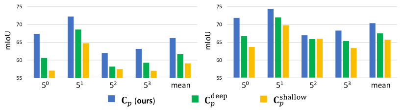
Figure 5: Ablation study on hypercorrelations on PASCAL-5ⁱ [61] dataset in 1-shot (left) and 5-shot (right) mIoU results.

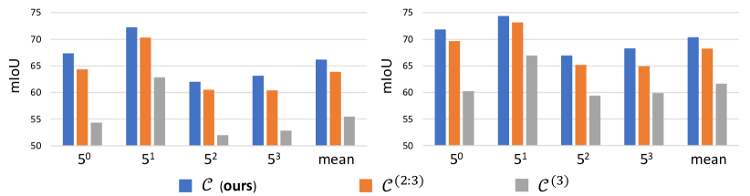
Figure 6: Ablation study on pyramid layers on PASCAL-5ⁱ [61] dataset in 1-shot (left) and 5-shot (right) mIoU results.

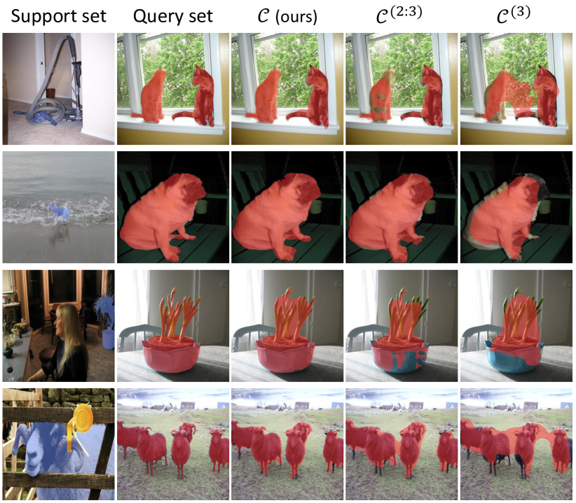
Figure 7: Ablation study on hypercorrelation pyramid layers.

Kernel type	1-shot					5-shot					# learnable params	time	memory footprint	FLOPs
	50	51	52	53	mean	50	51	52	53	mean		(ms)	(GB)	(G)
Original 4D kernel [58]	64.5	71.4	62.3	61.7	64.9	70.8	74.8	67.4	67.5	70.1	11.3M	512.17	4.12	702.35
Separable 4D kernel [81]	66.1	72.0	63.2	62.6	65.9	71.2	74.1	67.2	68.1	70.2	4.4M	28.48	1.50	28.40
Center-pivot 4D kernel (ours)	67.3	72.3	62.0	63.1	66.2	71.8	74.4	67.0	68.3	70.4	2.6M	25.51	1.39	20.56

Table 5: Comparison between three different 4D conv kernels in model size, per-episode inference time, memory consumption and FLOPs. For fair comparison, the inference times of all the models are measured on a machine with an Intel i7-7820X and an NVIDIA Titan-XP.

Ablation study on pyramid layers. To see the impact of hypercorrelation $\mathbf{C}_{p}$ at each layer $p$, we perform experiments in absence of each pyramidal layer. We train and evaluate our model using two different hypercorrelation pyramids, $\mathcal{C}^{(2:3)}=\{\mathbf{C}_{2},\mathbf{C}_{3}\}$ and $\mathcal{C}^{(3)}=\{\mathbf{C}_{3}\}$, and compare the results with ours $\mathcal{C}=\{\mathbf{C}_{p}\}_{p=1}^{3}$. Figure 6 summarizes the results; given hypercorrelation pyramid without geometric information ($\mathcal{C}^{(2:3)}$), our model fails to refine object boundaries in the final mask prediction as visualized in Fig. 7. Given a single hypercorrelation that only encodes semantic relations ($\mathcal{C}^{(3)}$), the model predictions are severely damaged, providing only rough localization of the target objects. These results indicate that capturing patterns of both semantic and geometric cues is essential for fine-grained localization.

Comparison between three different 4D kernels. We conduct ablation study on 4D kernel by replacing the proposed center-pivot 4D kernel with the original [58] and spatially separable [81] 4D kernels and compare their model size, per-episode inference time (1-shot), memory consumption, and floating point operations per second (FLOPs) with ours. Table 5 summarizes the results. The proposed kernel records the fastest inference time with the smallest memory/FLOPs requirements while being comparably effective than the other two. The results clearly support our claim that a large part of parameters in a high-dimensional kernel can safely be discarded without harming the quality of predictions; only a few relevant parameters are sufficient and even better for the purpose. While both the separable [81] and our center-pivot 4D convolutions operate on two separate 2D convolutions, auxiliary transformation layers with multiple batch normalizations that make the separable 4D conv numerically stable in its sequential design result in twice larger number of parameters (4.4M vs. 2.6M) and slower inference time (28.48ms vs. 25.51ms) than ours.

The number of 4D layers in building blocks. We also perform experiments with varying number of 4D conv layers in the two building blocks: $f_{p}^{\text{sqz}}$ and $f_{p}^{\text{mix}}$. Figure 8 plots 1-shot and 5-shot mIoU results on PASCAL-5ⁱ with the model sizes. In the experiments, appending additional 4D layers (with a group norm and a ReLU activation) in the building blocks provides clear performance improvements up to three layers but the accuracy eventually saturates after all. Hence we use a stack of three 4D layers for both.

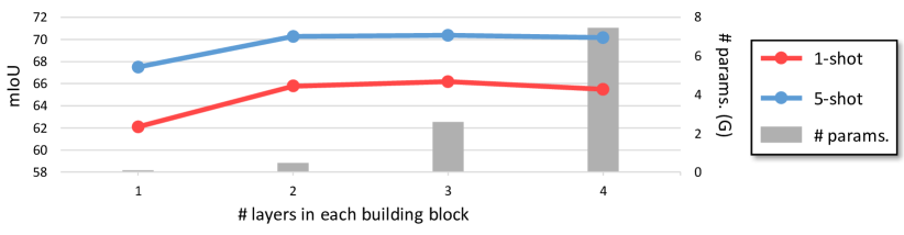
Figure 8: The effect of depths in building blocks: $f_{p}^{\text{sqz}}$ and $f_{p}^{\text{mix}}$.

Finetuning backbone networks. To investigate the significance of learning ‘feature correlations’ over learning ‘feature representation’ in few-shot regime, we finetune our backbone network and compare learning processes of the finetuned model and ours (frozen backbone). Figure 9 plots the training/validation curves of the finetuned model and ours on every fold of PASCAL-5ⁱ. The finetuned model rapidly overfits to the training data, losing generic, comprehensive visual representations learned from large-scale dataset [9]. Meanwhile, our model with frozen backbone provides better generalizibility with large trade-offs between training and validation accuracies. The results reveal that learning new appearances under limited supervision requires understanding their ‘relations’ to diverse visual patterns acquired from a vast amount of past experiences, e.g., ImageNet classification. This is quite analogous to human vision perspective in the sense that we generalize novel concepts (what we see) by analyzing their relations to the past observations (what we know) [40].

For additional experimental details, results and analyses, we refer the readers to the Appendix.

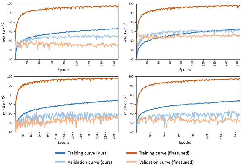
Figure 9: Learning curves (x-axis: epoch, y-axis: mIoU) on PASCAL-5ⁱ. We carefully tuned the learning rate of the backbone and set it to 100 times smaller than the layers in HSNet (1e-5).

6 Conclusion

We have presented a novel framework that analyzes complex feature correlations in a fully-convolutional manner using light-weight 4D convolutions. The significant performance improvements on three standard benchmarks demonstrate that learning patterns of feature relations from multiple visual aspects is effective in fine-grained segmentation under limited supervision. We also demonstrated a unique way of discarding insignificant weights leads to an efficient decomposition of a 4D kernel into a pair of 2D kernels, thus allowing extensive use of 4D conv layers at a significantly small cost. We believe our investigation will further facilitate the use of 4D convolutions in other domains that require learning to analyze high-dimensional correlations.

Acknowledgements. This work was supported by Samsung Advanced Institute of Technology (SAIT), the NRF grant (NRF-2017R1E1A1A01077999), and the IITP grant (No.2019-0-01906, AI Graduate School Program - POSTECH) funded by Ministry of Science and ICT, Korea.

Appendix A Complete derivation of the center-pivot 4D convolution

In this section, we extend Sec. 4.4 to provide a complete derivation of the center-pivot 4D convolution. Note that a typical 4D convolution parameterized by a kernel ${k}\in\mathbb{R}^{\hat{k}\times\hat{k}\times\hat{k}\times\hat{k}}$ on a correlation tensor $c\in\mathbb{R}^{H\times W\times H\times W}$ at position $(\mathbf{x},\mathbf{x}^{\prime})\in\mathbb{R}^{4}$ is formulated as

$$({c}*{k})(\mathbf{x},\mathbf{x}^{\prime}) =\sum_{(\mathbf{p},\mathbf{p}^{\prime})\in\mathcal{P}(\mathbf{x},\mathbf{x}^{\prime})}{c}(\mathbf{p},\mathbf{p}^{\prime}){k}(\mathbf{p}-\mathbf{x},\mathbf{p}^{\prime}-\mathbf{x}^{\prime}),$$ (6)

where $\mathcal{P}(\mathbf{x},\mathbf{x}^{\prime})$ denotes a set of neighbourhood regions within the local 4D window centered on position $(\mathbf{x},\mathbf{x}^{\prime})$, i.e., $\mathcal{P}(\mathbf{x},\mathbf{x}^{\prime})=\mathcal{P}(\mathbf{x})\times\mathcal{P}(\mathbf{x}^{\prime})$ as visualized in Fig. 4. Now we design a light-weight, efficient 4D convolution via a reasonable weight-sparsification; from a set of neighborhood positions within a local 4D window of interest, our kernel aims to disregard a large number of activations located at fairly insignificant positions in the 4D window, thereby focusing only on a small subset of relevant activations for capturing complex patterns in the correlation tensor. Specifically, we consider activations at positions that pivots either one of 2-dimensional centers, e.g., $\mathbf{x}$ or $\mathbf{x}^{\prime}$, as the foremost influential ones. Given 4D position $(\mathbf{x},\mathbf{x}^{\prime})$, we collect its neighbors if and only if they are adjacent to either $\mathbf{x}$ or $\mathbf{x}^{\prime}$ in its corresponding 2D subspace and define two respective sets as

$$\mathcal{P}_{c}(\mathbf{x},\mathbf{x}^{\prime})=\{(\mathbf{p},\mathbf{p}^{\prime})\in\mathcal{P}(\mathbf{x},\mathbf{x}^{\prime}):\mathbf{p}=\mathbf{x}\},$$ (7)

and

$$\mathcal{P}_{c^{\prime}}(\mathbf{x},\mathbf{x}^{\prime})=\{(\mathbf{p},\mathbf{p}^{\prime})\in\mathcal{P}(\mathbf{x},\mathbf{x}^{\prime}):\mathbf{p}^{\prime}=\mathbf{x}^{\prime}\}.$$ (8)

The set of center-pivot neighbours $\mathcal{P}_{\text{CP}}(\mathbf{x},\mathbf{x}^{\prime})$ is defined as a union of the two subsets:

$$\mathcal{P}_{\text{CP}}(\mathbf{x},\mathbf{x}^{\prime})=\mathcal{P}_{c}(\mathbf{x},\mathbf{x}^{\prime})\cup\mathcal{P}_{c^{\prime}}(\mathbf{x},\mathbf{x}^{\prime}).$$ (9)

Based on this small subset of neighbors, center-pivot 4D (CP 4D) convolution can be formulated as a union of two separate 4D convolutions:

$$(c*k_{\text{CP}})(\mathbf{x},\mathbf{x}^{\prime}) =(c*k_{c})(\mathbf{x},\mathbf{x}^{\prime})+(c*k_{c^{\prime}})(\mathbf{x},\mathbf{x}^{\prime}),$$ (10)

where $k_{c}$ and $k_{c^{\prime}}$ are 4D kernels with their respective neighbours $\mathcal{P}_{c}(\mathbf{x},\mathbf{x}^{\prime})$ and $\mathcal{P}_{c^{\prime}}(\mathbf{x},\mathbf{x}^{\prime})$. Now consider below

$$(c*k_{c})(\mathbf{x},\mathbf{x}^{\prime}) =\sum_{(\mathbf{p},\mathbf{p}^{\prime})\in\mathcal{P}_{c}(\mathbf{x},\mathbf{x}^{\prime})}{c}(\mathbf{p},\mathbf{p}^{\prime}){k}(\mathbf{p}-\mathbf{x},\mathbf{p}^{\prime}-\mathbf{x}^{\prime})$$

$$=\sum_{\mathbf{p}^{\prime}\in\mathcal{P}(\mathbf{x}^{\prime})}{c}(\mathbf{x},\mathbf{p}^{\prime}){k}(\mathbf{x}-\mathbf{x},\mathbf{p}^{\prime}-\mathbf{x}^{\prime})$$

$$=\sum_{\mathbf{p}^{\prime}\in\mathcal{P}(\mathbf{x}^{\prime})}{c}(\mathbf{x},\mathbf{p}^{\prime}){k}(\mathbf{0},\mathbf{p}^{\prime}-\mathbf{x}^{\prime})$$

$$=\sum_{\mathbf{p}^{\prime}\in\mathcal{P}(\mathbf{x}^{\prime})}{c}(\mathbf{x},\mathbf{p}^{\prime}){k}_{c}^{\textrm{2D}}(\mathbf{p}^{\prime}-\mathbf{x}^{\prime}),$$ (11)

which is equivalent to convolution with kernel $k_{c}^{\mathrm{2D}}=k(\mathbf{0},:)\in\mathbb{R}^{\hat{k}\times\hat{k}}$ performed on 2D slice of the 4D tensor $c(\mathbf{x},\ :)$. Similarly,

$$(c*k_{c^{\prime}})(\mathbf{x},\mathbf{x}^{\prime}) =\sum_{(\mathbf{p},\mathbf{p}^{\prime})\in\mathcal{P}_{c^{\prime}}(\mathbf{x},\mathbf{x}^{\prime})}{c}(\mathbf{p},\mathbf{p}^{\prime}){k}(\mathbf{p}-\mathbf{x},\mathbf{p}^{\prime}-\mathbf{x}^{\prime})$$

$$=\sum_{\mathbf{p}\in\mathcal{P}(\mathbf{x})}{c}(\mathbf{p},\mathbf{x}^{\prime}){k}(\mathbf{p}-\mathbf{x},\mathbf{x}^{\prime}-\mathbf{x}^{\prime})$$

$$=\sum_{\mathbf{p}\in\mathcal{P}(\mathbf{x})}{c}(\mathbf{p},\mathbf{x}^{\prime}){k}(\mathbf{p}-\mathbf{x},\mathbf{0})$$

$$=\sum_{\mathbf{p}\in\mathcal{P}(\mathbf{x})}{c}(\mathbf{p},\mathbf{x}^{\prime}){k}_{c^{\prime}}^{\textrm{2D}}(\mathbf{p}-\mathbf{x}),$$ (12)

where $k_{c^{\prime}}^{\mathrm{2D}}=k(:,\mathbf{0})\in\mathbb{R}^{\hat{k}\times\hat{k}}$. Based on above derivations, we rewrite Eqn. 10 as follows

$$(c*k_{\text{CP}})(\mathbf{x},\mathbf{x}^{\prime})=\sum_{\mathbf{p}^{\prime}\in\mathcal{P}(\mathbf{x}^{\prime})} {c}(\mathbf{x},\mathbf{p}^{\prime}){k}_{c}^{\textrm{2D}}(\mathbf{p}^{\prime}-\mathbf{x}^{\prime})$$

$$+\sum_{\mathbf{p}\in\mathcal{P}(\mathbf{x})} {c}(\mathbf{p},\mathbf{x}^{\prime}){k}_{c^{\prime}}^{\textrm{2D}}(\mathbf{p}-\mathbf{x}),$$ (13)

which performs two different convolutions on separate 2D subspaces, having a linear complexity.

Appendix B Implementation details

For the backbone networks, we employ VGG [64] and ResNet [17] families pre-trained on ImageNet [9], e.g., VGG16, ResNet50, and ResNet101. For the VGG16 backbone, we extract features after every conv layer in the last two building blocks: from conv4_x to conv5_x, and after the last maxpooling layer. For the ResNet backbones, we extract features at the end of each bottleneck before ReLU activation: from conv3_x to conv5_x. This feature extracting scheme results in 3 pyramidal layers ($P=3$) for every backbone. We set spatial sizes of both support and query images to $400\times 400$, i.e., $H,W=400$, thus having $H_{1},W_{1}=50$, $H_{2},W_{2}=25$, and $H_{3},W_{3}=13$ for both ResNet50 and ResNet101 bakcbones and $H_{1},W_{1}=50$, $H_{2},W_{2}=25$, and $H_{3},W_{3}=12$ for the VGG16 backbone. The network is implemented in PyTorch [51] and optimized using Adam [24] with learning rate of 1e-3. We train our model with batch size of 20, 40, and 20 for PASCAL-5ⁱ, COCO-20ⁱ, and FSS-1000 respectively. We freeze the pre-trained backbone networks to prevent them from learning class-specific representations of the training data. The intermediate tensor dimensions, the number of parameters of each layers and other additional details of the network are demonstrated in Tab. A5, A6, and A7 for respective backbones of VGG16, ResNet50, and ResNet101.

Backbone network	Methods	1-shot						5-shot						# learnable
		$5^{0}$	$5^{1}$	$5^{2}$	$5^{3}$	mIoU	FB-IoU	$5^{0}$	$5^{1}$	$5^{2}$	$5^{3}$	mIoU	FB-IoU	params
VGG16 [64]	SG-One [89]	40.2	58.4	48.4	38.4	46.3	63.1	41.9	58.6	48.6	39.4	47.1	65.9	19.0M
	CRNet [36]	-	-	-	-	55.2	66.4	-	-	-	-	58.5	71.0	-
	HSNet (ours)	53.6	61.7	55.0	50.3	55.2	70.5	58.3	64.7	58.9	54.6	59.1	73.5	2.6M
ResNet50 [17]	CANet [87]	52.5	65.9	51.3	51.9	55.4	66.2	55.5	67.8	51.9	53.2	57.1	69.6	19.0M
	RPMM [80]	55.2	66.9	52.6	50.7	56.3	-	56.3	67.3	54.5	51.0	57.3	-	19.7M
	CRNet [36]	-	-	-	-	55.7	66.8	-	-	-	-	58.8	71.5	-
	HSNet (ours)	57.4	66.8	55.8	56.5	59.1	73.8	62.6	69.2	62.5	62.4	64.2	77.4	2.6M
ResNet101 [17]	HSNet (ours)	60.1	67.8	57.3	59.0	61.1	74.4	63.9	69.9	62.0	63.6	64.8	77.1	2.6M

Table A1: Evaluation results on PASCAL-5ⁱ [61] benchmark in mIoU and FB-IoU evaluation metrics without the use of ignore_label. The results of other methods are from [36, 37, 70, 74, 80].

Appendix C Additional results and analyses

Additional $K$-shot results. Following the work of [4, 70, 80], we conduct $K$-shot experiments with $K\in\{1,5,10\}$. Table A2 compares our results with the recent methods [4, 70, 80] on PASCAL-5ⁱ and COCO-20ⁱ. The significant performance improvements on both datasets clearly indicate the effectiveness of our approach. Achieving 2.5%p and 4.6%p mIoU improvements over the previous best method [4] on respective PASCAL-5ⁱ and COCO-20ⁱ, our model again sets a new state of the art in 10-shot setting as well, showing notable improvements with larger $K$.

Numerical comparisons of ablation study. We tabularize Figures 5 and 6, e.g., ablation study on hypercorrelations and pyramidal layers, in Tables A3 and A4 respectively. Achieving 4.5%p mIoU improvements over $\mathbf{C}_{p}^{\text{deep}}$, our method clearly benefits from diverse feature correlations from multi-level CNN layers ($\mathbf{C}_{p}$) as seen in Tab. A3. A large performance gap between $\mathcal{C}^{(2:3)}$ and $\mathcal{C}^{(3)}$ in Tab. A4 (63.9 vs. 55.5) reveals that the intermediary second pyramidal layer ($p=2$) is especially effective in robust mask prediction compared to the first pyramidal layer ($p=1$).

Method	PASCAL-5i			COCO-20i
	1-shot	5-shot	10-shot	1-shot	5-shot	10-shot
RPMM [80]	56.3	57.3	57.6	30.6	35.5	33.1
PFENet [70]	60.8	61.9	62.1	35.8	39.0	39.7
RePRI [4]	59.7	66.6	68.1	34.1	41.6	44.1
HSNet (ours)	64.0	69.5	70.6	39.2	46.9	48.7

Table A2: Results on $K$-shot with ResNet50 backbone network where $K\in\{1,5,10\}$. The results of other methods are from [4].

Methods	1-shot					5-shot
	$5^{0}$	$5^{1}$	$5^{2}$	$5^{3}$	mean	$5^{0}$	$5^{1}$	$5^{2}$	$5^{3}$	mean
$\mathbf{C}_{p}^{\text{shallow}}$	57.1	64.7	57.5	57.0	59.1	63.7	69.8	66.0	63.4	65.7
$\mathbf{C}_{p}^{\text{deep}}$	60.6	68.6	58.2	59.2	61.7	66.7	72.0	65.9	65.4	67.5
$\mathbf{C}_{p}$ (ours)	67.3	72.3	62.0	63.1	66.2	71.8	74.4	67.0	68.3	70.4

Table A3: Numerical results of Figure 5. All experiments are performed with ResNet101 backbone [17].

Methods	1-shot					5-shot
	$5^{0}$	$5^{1}$	$5^{2}$	$5^{3}$	mean	$5^{0}$	$5^{1}$	$5^{2}$	$5^{3}$	mean
$\mathcal{C}^{(3)}$	54.3	62.8	52.0	52.8	55.5	60.2	67.0	59.4	59.9	61.6
$\mathcal{C}^{(2:3)}$	64.3	70.3	60.5	60.4	63.9	69.7	73.2	65.2	64.9	68.2
$\mathcal{C}$ (ours)	67.3	72.3	62.0	63.1	66.2	71.8	74.4	67.0	68.3	70.4

Table A4: Numerical results of Figure 6. All experiments are performed with ResNet101 backbone [17].

Evaluation results without using ignore_label on PASCAL-5ⁱ. The benchmarks of PASCAL-5ⁱ [61], COCO-20ⁱ [35], and FSS-1000 [33] consist of segmentation mask annotations in which each pixel is labeled with either background or one of the predefined object categories. As pixel-wise segmentation near object boundaries is ambiguous to perform even for human annotators, PASCAL-5ⁱ uses a special kind of label called ignore_label which marks pixel regions ignored during training and evaluation to mitigate the ambiguity.

Most recent few-shot segmentation work [4, 37, 46, 54, 61, 63, 70, 74, 75, 86] adopt this evaluation criteria but we found that some methods [36, 80, 87, 89] do not utilize ignore_label in their evaluations. Therefore, the methods are unfairly evaluated as fine-grained mask prediction near object boundaries is one of the most challenging part in segmentation problem. For fair comparisons, we intentionally exclude the methods of [36, 80, 87, 89] from Tab. 1 and compare the results of our model evaluated without the use of ignore_label with those methods [36, 80, 87, 89]. The results are summarized in Tab. A1. Even without using ignore_label, the proposed method sets a new state of the art with ResNet50 backbone, outperforming the previous best methods of [80] and [36] by (1-shot) 2.8%p and (5-shot) 5.4%p respectively. With VGG16 backbone, our method performs comparably effective to the previous best method [36] while having the smallest learnable parameters.

Appendix D Qualitative results

Results without support feature masking. As demonstrated in Sec. 5.1, we conduct experiments without support feature masking (Eqn. 1), similarly to co-segmentation problem with stronger demands for generalizibility. Figure A1 visualizes some example results on PASCAL-5ⁱ dataset. Even without the use of support masks (in both training and testing), our model effectively segments target instances in query images. The results indicate that learning patterns of feature correlations from multiple visual aspects is effective in fine-grained segmentation as well as identifying ‘common’ instances in the support and query images.

Additional qualitative results. We present additional qualitative results on PASCAL-5ⁱ [61], COCO-20ⁱ [46], and FSS-1000 [33] benchmark datasets. All the qualitative results are best viewed in electronic forms. Example results in presence of large scale-differences, truncations, and occlusions are shown in Fig. A2, A3, and A4. Figure A5 visualizes model predictions under large illumination-changes in support and query images. Figure A6 visualizes some sample predictions given exceptionally small objects in either support or query images. As seen in Fig. A7, we found that our model sometimes predicts more reliable segmentation masks than ground-truth ones. Some qualitative results in presence of large intra-class variations and noisy clutters in background are shown in Fig. A8 and A9. Given only a single support image-annotation pair, our model effectively segments multiple instances in a query image as visualized in Fig. A10. Figure A11 shows representative failure cases; our model fails to localize target objects in presence of severe occlusions, intra-class variances and extremely tiny support (or query) objects. As seen in Fig. A12, the model predictions become much reliable given multiple support image-mask pairs, i.e., $K>1$.

The code and data to reproduce all experiments in this paper is available at our project page: http://cvlab.postech.ac.kr/research/HSNet/.

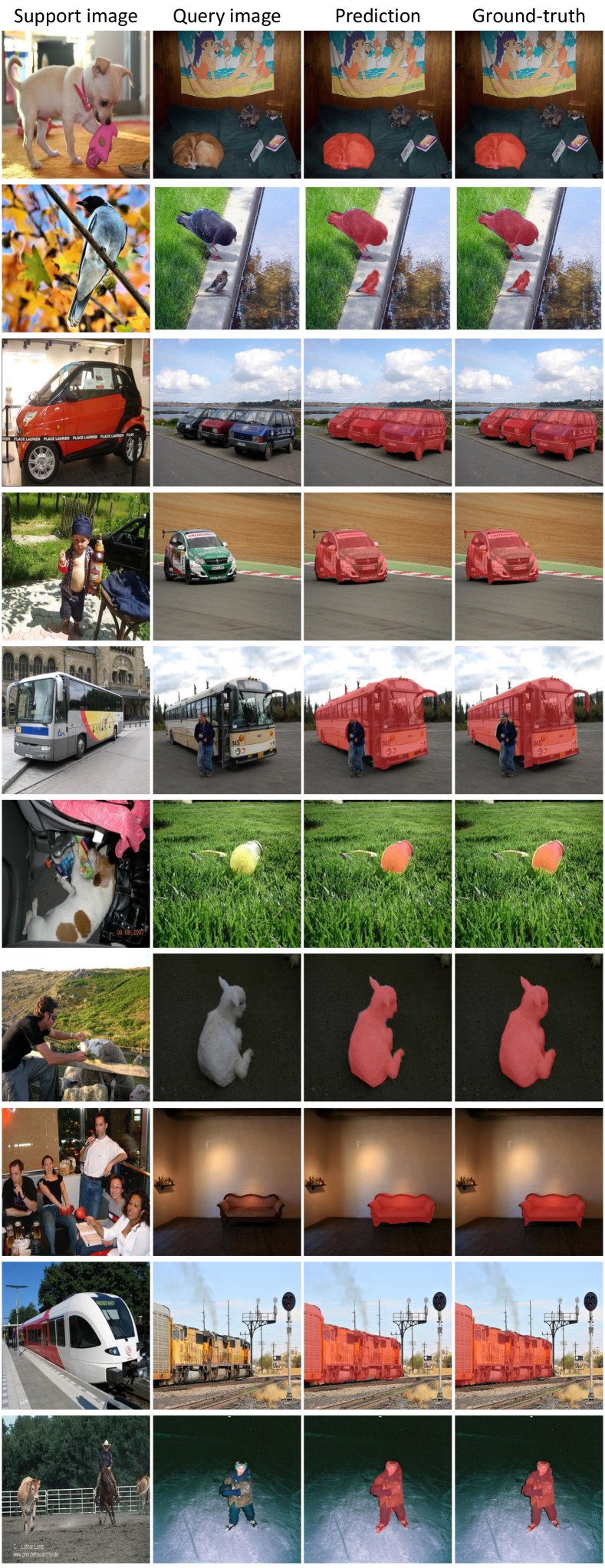
Figure A1: Example results without support feature masking (Eqn. 1) on PASCAL-5ⁱ dataset.

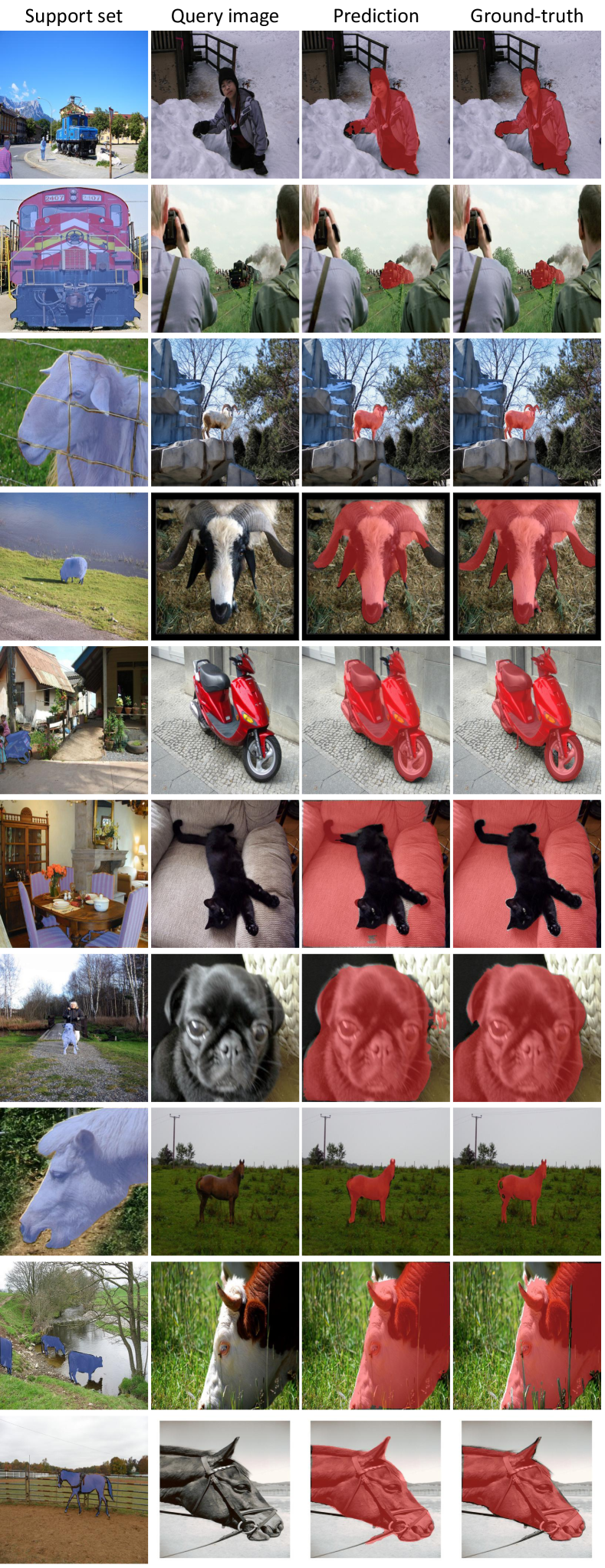
Figure A2: Qualitative (1-shot) results on PASCAL-5ⁱ [61] dataset under large differences in object scales.

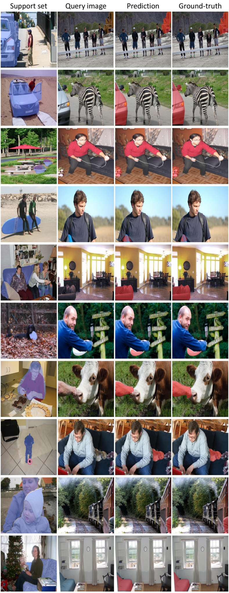
Figure A3: Qualitative (1-shot) results on PASCAL-5ⁱ [61] and COCO-20ⁱ [35] datasets under large truncations and occlusions.

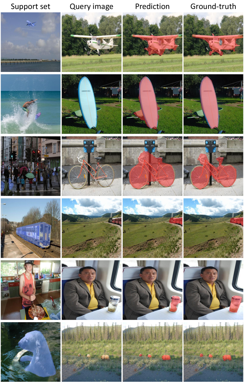
Figure A4: Qualitative (1-shot) results on COCO-20ⁱ [35] dataset under large differences in object scales.

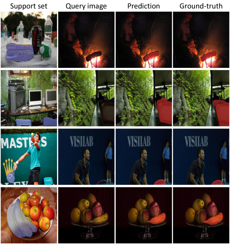
Figure A5: Qualitative (1-shot) results on COCO-20ⁱ [35] dataset under large illumination-changes in support and query images.

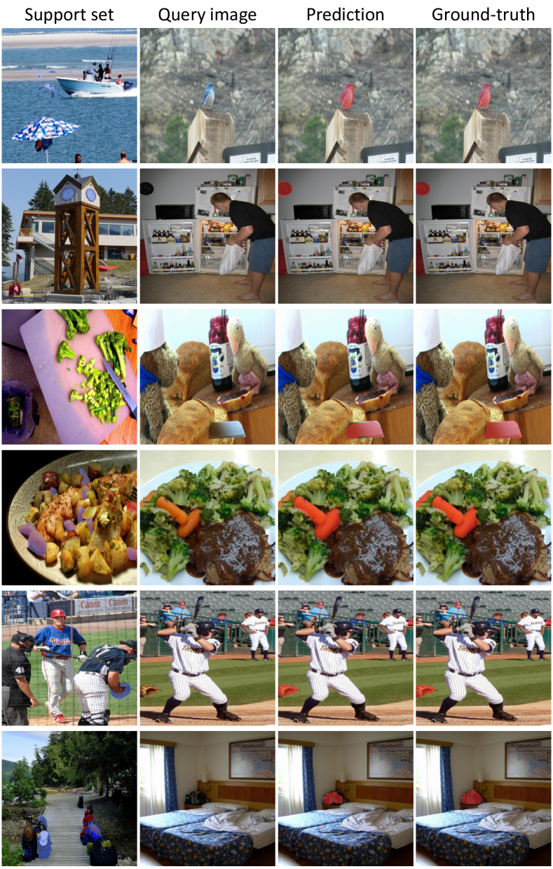
Figure A6: Qualitative (1-shot) results on COCO-20ⁱ [35] dataset with exceptionally small objects.

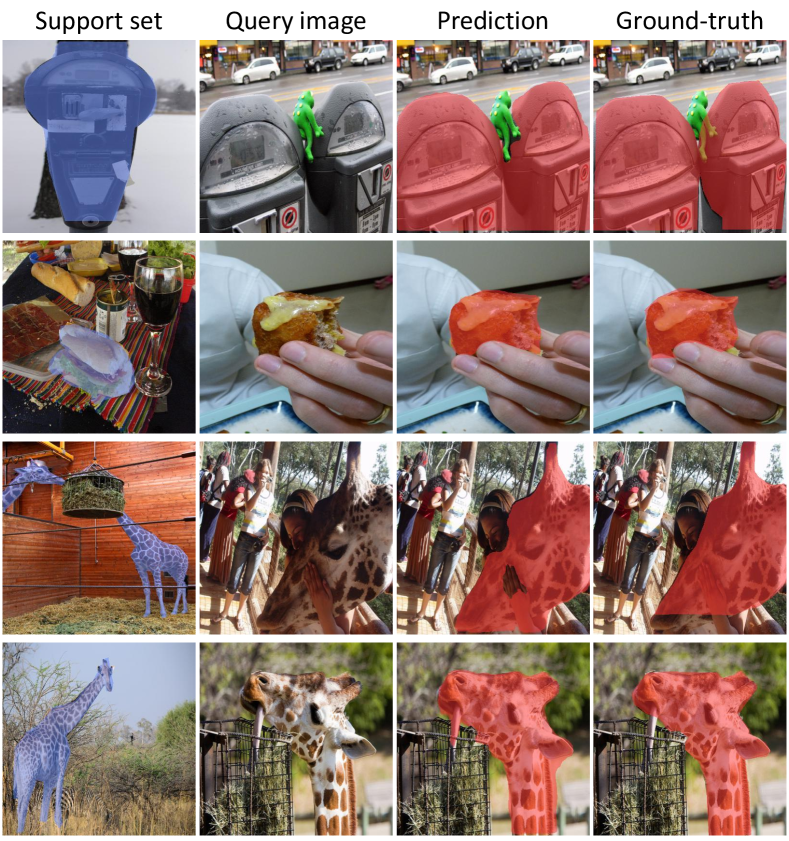
Figure A7: Our network occasionally predicts more accurate segmentation masks than human-annotated ground-truths.

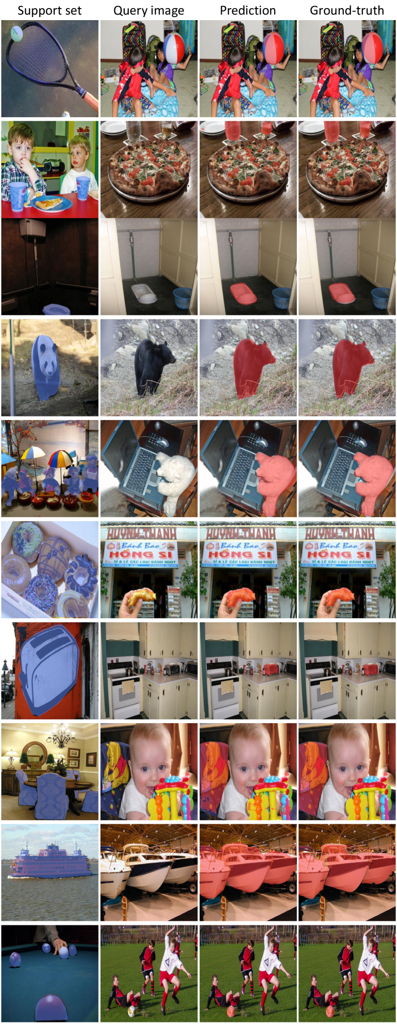
Figure A8: Qualitative (1-shot) results on PASCAL-5ⁱ [61] and COCO-20ⁱ [35] datasets under large intra-class variations.

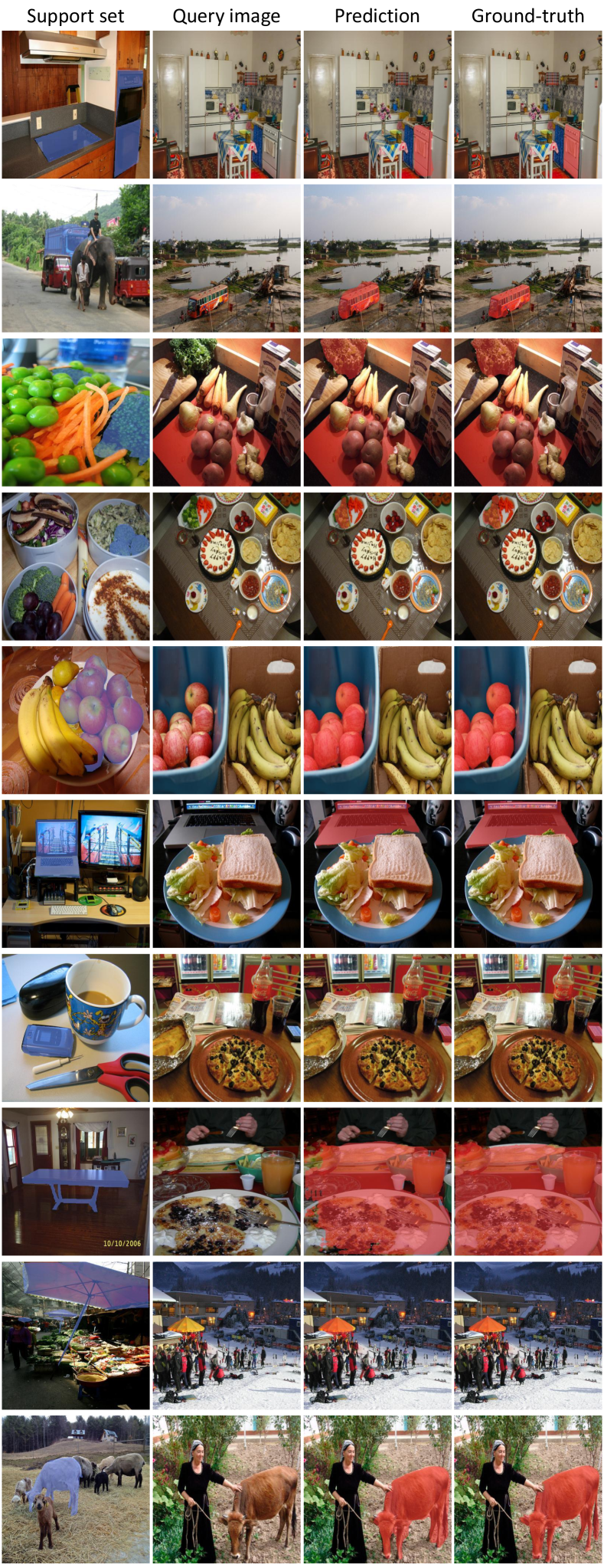
Figure A9: Qualitative (1-shot) results on PASCAL-5ⁱ [61] and COCO-20ⁱ [35] datasets in presence of noisy background clutters.

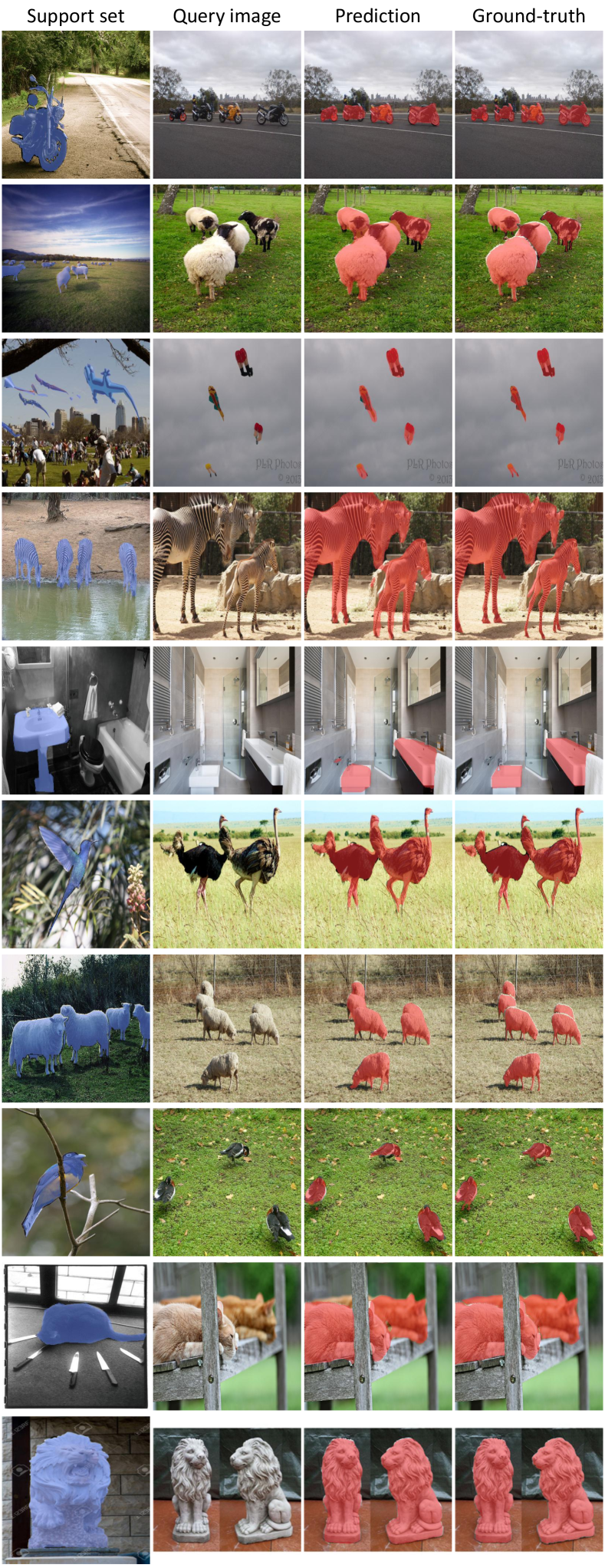
Figure A10: One-to-many and many-to-many (1-shot) results on PASCAL-5ⁱ [61], COCO-20ⁱ [35], and FSS-1000 [33] datasets.

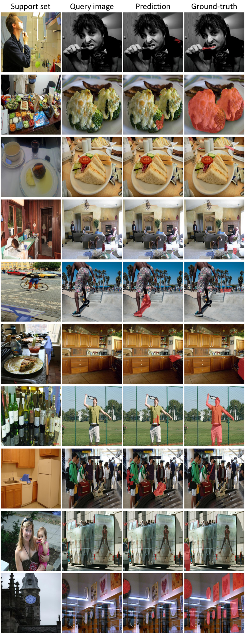
Figure A11: Representative failure cases in presence of severe occlusions, intra-class variances and extremely tiny objects.

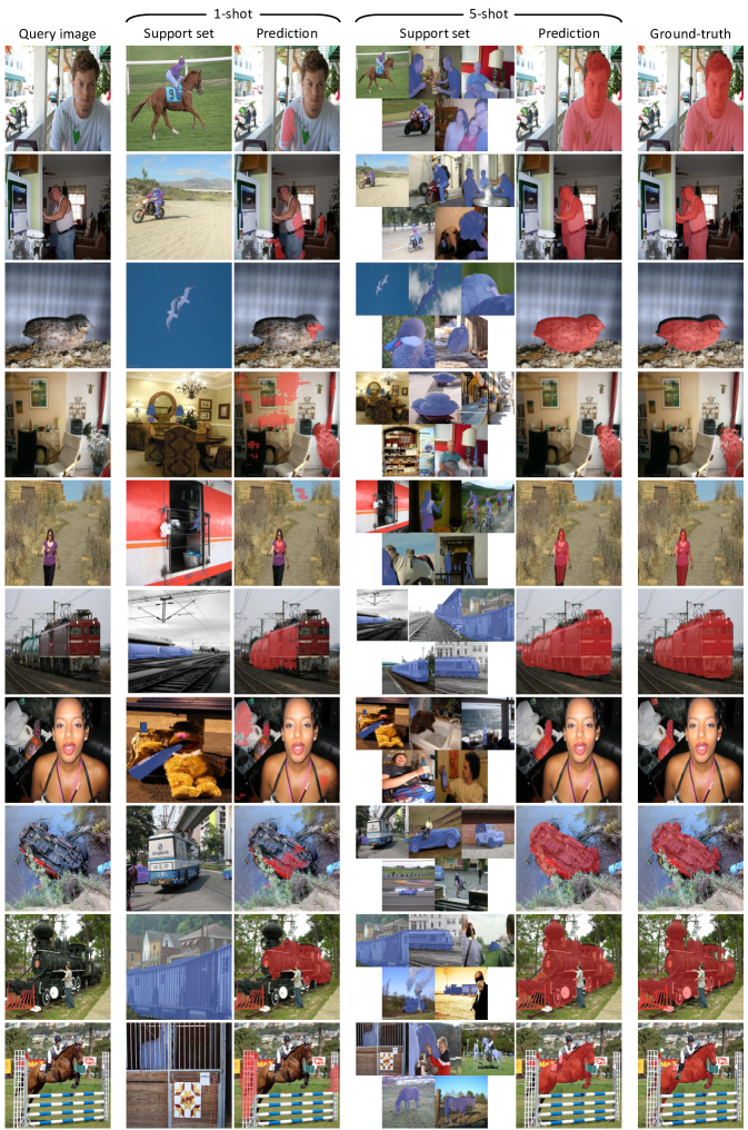
Figure A12: Comparison between 1-shot and 5-shot results on PASCAL-5ⁱ dataset [61]. Multiple support images and mask annotations clearly help our model generate accurate mask predictions on query images in many challenging cases.

Layer	Input		Output		Operation	# params.
VGG16 Backbone	$I^{\mathrm{q}}$	(3, 400, 400)	$\{\mathbf{F}_{l}^{\mathrm{q}}\}_{l=1}^{7}$	(512, 12, 12) $\times$ 1	Series of 2D Convs	14.7M (frozen)
				(512, 25, 25) $\times$ 3
				(512, 50, 50) $\times$ 3
	$I^{\mathrm{s}}$	(3, 400, 400)	$\{\mathbf{F}_{l}^{\mathrm{s}}\}_{l=1}^{7}$	(512, 12, 12) $\times$ 1
				(512, 25, 25) $\times$ 3
				(512, 50, 50) $\times$ 3
Masking Layer	$\{\mathbf{F}_{l}^{\mathrm{s}}\}_{l=1}^{7}$	(512, 12, 12) $\times$ 1	$\{\hat{\mathbf{F}}_{l}^{\mathrm{s}}\}_{l=1}^{7}$	(512, 12, 12) $\times$ 1 (512, 25, 25) $\times$ 3 (512, 50, 50) $\times$ 3	Bilinear Interpolation Hadamard Product	-
		(512, 25, 25) $\times$ 3
		(512, 50, 50) $\times$ 3
	$\mathbf{M}^{\mathrm{s}}$	(1, 400, 400)
Correlation Layer	$\{\mathbf{F}_{l}^{\mathrm{q}}\}_{l=1}^{7}$	(512, 12, 12) $\times$ 1	$\{\mathbf{C}_{p}\}_{p=1}^{3}$	(1, 12, 12, 12, 12) (3, 25, 25, 25, 25) (3, 50, 50, 50, 50)	Cosine Similarity	-
		(512, 25, 25) $\times$ 3
		(512, 50, 50) $\times$ 3
	$\{\hat{\mathbf{F}}_{l}^{\mathrm{s}}\}_{l=1}^{7}$	(512, 12, 12) $\times$ 1
		(512, 25, 25) $\times$ 3
		(512, 50, 50) $\times$ 3
Squeezing Block $f_{3}^{\text{sqz}}$	$\mathbf{C}_{3}$	(1, 12, 12, 12, 12)	$\mathbf{C}_{3}^{\text{sqz}}$	(128, 12, 12, 2, 2)	$\begin{pmatrix}\textsc{CP 4D conv}\\ \textsc{Group Norm}\\ \textsc{ReLU}\end{pmatrix}\times 3$	167K
Squeezing Block $f_{2}^{\text{sqz}}$	$\mathbf{C}_{2}$	(3, 25, 25, 25, 25)	$\mathbf{C}_{2}^{\text{sqz}}$	(128, 25, 25, 2, 2)	$\begin{pmatrix}\textsc{CP 4D conv}\\ \textsc{Group Norm}\\ \textsc{ReLU}\end{pmatrix}\times 3$	169K
Squeezing Block $f_{1}^{\text{sqz}}$	$\mathbf{C}_{1}$	(3, 50, 50, 50, 50)	$\mathbf{C}_{1}^{\text{sqz}}$	(128, 50, 50, 2, 2)	$\begin{pmatrix}\textsc{CP 4D conv}\\ \textsc{Group Norm}\\ \textsc{ReLU}\end{pmatrix}\times 3$	202K
Mixing Block $f_{2}^{\text{mix}}$			$\mathbf{C}_{2}^{\text{mix}}$	(128, 25, 25, 2, 2)	Bilinear Interpolation Element-wise Addition $\begin{pmatrix}\textsc{CP 4D conv}\\ \textsc{Group Norm}\\ \textsc{ReLU}\end{pmatrix}\times 3$	886K
	$\mathbf{C}_{3}^{\text{sqz}}$	(128, 12, 12, 2, 2)
	$\mathbf{C}_{2}^{\text{sqz}}$	(128, 25, 25, 2, 2)
Mixing Block $f_{1}^{\text{mix}}$			$\mathbf{C}_{1}^{\text{mix}}$	(128, 50, 50, 2, 2)	Bilinear Interpolation Element-wise Addition $\begin{pmatrix}\textsc{CP 4D conv}\\ \textsc{Group Norm}\\ \textsc{ReLU}\end{pmatrix}\times 3$	886K
	$\mathbf{C}_{2}^{\text{mix}}$	(128, 25, 25, 2, 2)
	$\mathbf{C}_{1}^{\text{sqz}}$	(128, 50, 50, 2, 2)
Pooling Layer	$\mathbf{C}_{1}^{\text{mix}}$	(128, 50, 50, 2, 2)	$\mathbf{Z}$	(128, 50, 50)	Average-pooling	-
Decoder Layer	$\mathbf{Z}$	(128, 50, 50)	$\mathbf{\hat{M}}^{\mathrm{q}}$	(2, 400, 400)	Series of 2D Convs with	259K
					Bilinear Interpolation

Table A5: Hypercorrelation Squeeze Networks (HSNet) with VGG16 [64] backbone network. The reported number of parameters in VGG16 backbone network (14.7M) excludes those in fully-connected layers (unused in our model). The total number of ‘learnable’ parameters amounts to 2.6M. The number of intermediate features extracted from backbone network amounts to 7, i.e., $L=7$. The CP 4D conv refers to the proposed center-pivot 4D convolution.

Layer	Input		Output		Operation	# params.
ResNet50 Backbone	$I^{\mathrm{q}}$	(3, 400, 400)	$\{\mathbf{F}_{l}^{\mathrm{q}}\}_{l=1}^{13}$	(2048, 13, 13) $\times$ 3	Series of 2D Convs	23.6M (frozen)
				(1024, 25, 25) $\times$ 6
				(512, 50, 50) $\times$ 4
	$I^{\mathrm{s}}$	(3, 400, 400)	$\{\mathbf{F}_{l}^{\mathrm{s}}\}_{l=1}^{13}$	(2048, 13, 13) $\times$ 3
				(1024, 25, 25) $\times$ 6
				(512, 50, 50) $\times$ 4
Masking Layer	$\{\mathbf{F}_{l}^{\mathrm{s}}\}_{l=1}^{13}$	(2048, 13, 13) $\times$ 3	$\{\hat{\mathbf{F}}_{l}^{\mathrm{s}}\}_{l=1}^{13}$	(2048, 13, 13) $\times$ 3 (1024, 25, 25) $\times$ 6 (512, 50, 50) $\times$ 4	Bilinear Interpolation Hadamard Product	-
		(1024, 25, 25) $\times$ 6
		(512, 50, 50) $\times$ 4
	$\mathbf{M}^{\mathrm{s}}$	(1, 400, 400)
Correlation Layer	$\{\mathbf{F}_{l}^{\mathrm{q}}\}_{l=1}^{13}$	(2048, 13, 13) $\times$ 3	$\{\mathbf{C}_{p}\}_{p=1}^{3}$	(3, 13, 13, 13, 13) (6, 25, 25, 25, 25) (4, 50, 50, 50, 50)	Cosine Similarity	-
		(1024, 25, 25) $\times$ 6
		(512, 50, 50) $\times$ 4
	$\{\hat{\mathbf{F}}_{l}^{\mathrm{s}}\}_{l=1}^{13}$	(2048, 13, 13) $\times$ 3
		(1024, 25, 25) $\times$ 6
		(512, 50, 50) $\times$ 4
Squeezing Block $f_{3}^{\text{sqz}}$	$\mathbf{C}_{3}$	(3, 13, 13, 13, 13)	$\mathbf{C}_{3}^{\text{sqz}}$	(128, 13, 13, 2, 2)	$\begin{pmatrix}\textsc{CP 4D conv}\\ \textsc{Group Norm}\\ \textsc{ReLU}\end{pmatrix}\times 3$	168K
Squeezing Block $f_{2}^{\text{sqz}}$	$\mathbf{C}_{2}$	(6, 25, 25, 25, 25)	$\mathbf{C}_{2}^{\text{sqz}}$	(128, 25, 25, 2, 2)	$\begin{pmatrix}\textsc{CP 4D conv}\\ \textsc{Group Norm}\\ \textsc{ReLU}\end{pmatrix}\times 3$	172K
Squeezing Block $f_{1}^{\text{sqz}}$	$\mathbf{C}_{1}$	(4, 50, 50, 50, 50)	$\mathbf{C}_{1}^{\text{sqz}}$	(128, 50, 50, 2, 2)	$\begin{pmatrix}\textsc{CP 4D conv}\\ \textsc{Group Norm}\\ \textsc{ReLU}\end{pmatrix}\times 3$	203K
Mixing Block $f_{2}^{\text{mix}}$			$\mathbf{C}_{2}^{\text{mix}}$	(128, 25, 25, 2, 2)	Bilinear Interpolation Element-wise Addition $\begin{pmatrix}\textsc{CP 4D conv}\\ \textsc{Group Norm}\\ \textsc{ReLU}\end{pmatrix}\times 3$	886K
	$\mathbf{C}_{3}^{\text{sqz}}$	(128, 13, 13, 2, 2)
	$\mathbf{C}_{2}^{\text{sqz}}$	(128, 25, 25, 2, 2)
Mixing Block $f_{1}^{\text{mix}}$			$\mathbf{C}_{1}^{\text{mix}}$	(128, 50, 50, 2, 2)	Bilinear Interpolation Element-wise Addition $\begin{pmatrix}\textsc{CP 4D conv}\\ \textsc{Group Norm}\\ \textsc{ReLU}\end{pmatrix}\times 3$	886K
	$\mathbf{C}_{2}^{\text{mix}}$	(128, 25, 25, 2, 2)
	$\mathbf{C}_{1}^{\text{sqz}}$	(128, 50, 50, 2, 2)
Pooling Layer	$\mathbf{C}_{1}^{\text{mix}}$	(128, 50, 50, 2, 2)	$\mathbf{Z}$	(128, 50, 50)	Average-pooling	-
Decoder Layer	$\mathbf{Z}$	(128, 50, 50)	$\mathbf{\hat{M}}^{\mathrm{q}}$	(2, 400, 400)	Series of 2D Convs with	259K
					Bilinear Interpolation

Table A6: Hypercorrelation Squeeze Networks (HSNet) with ResNet50 [17] backbone network. The reported number of parameters in ResNet50 backbone network (23.6M) excludes those in fully-connected layers (unused in our model). The total number of ‘learnable’ parameters amounts to 2.6M. The number of intermediate features extracted from backbone network amounts to 13, i.e., $L=13$.

Layer	Input		Output		Operation	# params.
ResNet101 Backbone	$I^{\mathrm{q}}$	(3, 400, 400)	$\{\mathbf{F}_{l}^{\mathrm{q}}\}_{l=1}^{30}$	(2048, 13, 13) $\times$ 3	Series of 2D Convs	42.6M (frozen)
				(1024, 25, 25) $\times$ 23
				(512, 50, 50) $\times$ 4
	$I^{\mathrm{s}}$	(3, 400, 400)	$\{\mathbf{F}_{l}^{\mathrm{s}}\}_{l=1}^{30}$	(2048, 13, 13) $\times$ 3
				(1024, 25, 25) $\times$ 23
				(512, 50, 50) $\times$ 4
Masking Layer	$\{\mathbf{F}_{l}^{\mathrm{s}}\}_{l=1}^{30}$	(2048, 13, 13) $\times$ 3	$\{\hat{\mathbf{F}}_{l}^{\mathrm{s}}\}_{l=1}^{30}$	(2048, 13, 13) $\times$ 3 (1024, 25, 25) $\times$ 23 (512, 50, 50) $\times$ 4	Bilinear Interpolation Hadamard Product	-
		(1024, 25, 25) $\times$ 23
		(512, 50, 50) $\times$ 4
	$\mathbf{M}^{\mathrm{s}}$	(1, 400, 400)
Correlation Layer	$\{\mathbf{F}_{l}^{\mathrm{q}}\}_{l=1}^{30}$	(2048, 13, 13) $\times$ 3	$\{\mathbf{C}_{p}\}_{p=1}^{3}$	(3, 13, 13, 13, 13) (23, 25, 25, 25, 25) (4, 50, 50, 50, 50)	Cosine Similarity	-
		(1024, 25, 25) $\times$ 23
		(512, 50, 50) $\times$ 4
	$\{\hat{\mathbf{F}}_{l}^{\mathrm{s}}\}_{l=1}^{30}$	(2048, 13, 13) $\times$ 3
		(1024, 25, 25) $\times$ 23
		(512, 50, 50) $\times$ 4
Squeezing Block $f_{3}^{\text{sqz}}$	$\mathbf{C}_{3}$	(3, 13, 13, 13, 13)	$\mathbf{C}_{3}^{\text{sqz}}$	(128, 13, 13, 2, 2)	$\begin{pmatrix}\textsc{CP 4D conv}\\ \textsc{Group Norm}\\ \textsc{ReLU}\end{pmatrix}\times 3$	168K
Squeezing Block $f_{2}^{\text{sqz}}$	$\mathbf{C}_{2}$	(23, 25, 25, 25, 25)	$\mathbf{C}_{2}^{\text{sqz}}$	(128, 25, 25, 2, 2)	$\begin{pmatrix}\textsc{CP 4D conv}\\ \textsc{Group Norm}\\ \textsc{ReLU}\end{pmatrix}\times 3$	185K
Squeezing Block $f_{1}^{\text{sqz}}$	$\mathbf{C}_{1}$	(4, 50, 50, 50, 50)	$\mathbf{C}_{1}^{\text{sqz}}$	(128, 50, 50, 2, 2)	$\begin{pmatrix}\textsc{CP 4D conv}\\ \textsc{Group Norm}\\ \textsc{ReLU}\end{pmatrix}\times 3$	203K
Mixing Block $f_{2}^{\text{mix}}$			$\mathbf{C}_{2}^{\text{mix}}$	(128, 25, 25, 2, 2)	Bilinear Interpolation Element-wise Addition $\begin{pmatrix}\textsc{CP 4D conv}\\ \textsc{Group Norm}\\ \textsc{ReLU}\end{pmatrix}\times 3$	886K
	$\mathbf{C}_{3}^{\text{sqz}}$	(128, 13, 13, 2, 2)
	$\mathbf{C}_{2}^{\text{sqz}}$	(128, 25, 25, 2, 2)
Mixing Block $f_{1}^{\text{mix}}$			$\mathbf{C}_{1}^{\text{mix}}$	(128, 50, 50, 2, 2)	Bilinear Interpolation Element-wise Addition $\begin{pmatrix}\textsc{CP 4D conv}\\ \textsc{Group Norm}\\ \textsc{ReLU}\end{pmatrix}\times 3$	886K
	$\mathbf{C}_{2}^{\text{mix}}$	(128, 25, 25, 2, 2)
	$\mathbf{C}_{1}^{\text{sqz}}$	(128, 50, 50, 2, 2)
Pooling Layer	$\mathbf{C}_{1}^{\text{mix}}$	(128, 50, 50, 2, 2)	$\mathbf{Z}$	(128, 50, 50)	Average-pooling	-
Decoder Layer	$\mathbf{Z}$	(128, 50, 50)	$\mathbf{\hat{M}}^{\mathrm{q}}$	(2, 400, 400)	Series of 2D Convs with	259K
					Bilinear Interpolation

Table A7: Hypercorrelation Squeeze Networks (HSNet) with ResNet101 [17] backbone network. The reported number of parameters in ResNet101 backbone network (42.6M) excludes those in fully-connected layers (unused in our model). The total number of ‘learnable’ parameters amounts to 2.6M. The number of intermediate features extracted from backbone network amounts to 30, i.e., $L=30$.

References

- [1] Kelsey Allen, Evan Shelhamer, Hanul Shin, and Joshua Tenenbaum. Infinite mixture prototypes for few-shot learning. In Proc. International Conference on Machine Learning (ICML), 2019.
- [2] Reza Azad, Abdur R Fayjie, Claude Kauffman, Ismail Ben Ayed, Marco Pedersoli1, and Jose Dolz1. On the texture bias for few-shot cnn segmentation. In Proc. Winter Conference on Applications of Computer Vision (WACV), 2021.
- [3] Vassileios Balntas, Karel Lenc, Andrea Vedaldi, and Krystian Mikolajczyk. Hpatches: A benchmark and evaluation of handcrafted and learned local descriptors. In Proc. IEEE Conference on Computer Vision and Pattern Recognition (CVPR), pages 5173–5182, 2017.
- [4] Malik Boudiaf, Hoel Kervadec, Ziko Imtiaz Masud, Pablo Piantanida, Ismail Ben Ayed, and Jose Dolz. Few-shot segmentation without meta-learning: A good transductive inference is all you need? In Proc. IEEE Conference on Computer Vision and Pattern Recognition (CVPR), 2021.
- [5] Fabio Cermelli, Massimiliano Mancini, Samuel Rota Bulo, Elisa Ricci, and Barbara Caputo. Modeling the background for incremental learning in semantic segmentation. In Proc. IEEE Conference on Computer Vision and Pattern Recognition (CVPR), 2020.
- [6] Yu-Ting Chang, Qiaosong Wang, Wei-Chih Hung, Robinson Piramuthu, Yi-Hsuan Tsai, and Ming-Hsuan Yang. Weakly-supervised semantic segmentation via sub-category exploration. In Proc. IEEE Conference on Computer Vision and Pattern Recognition (CVPR), 2020.
- [7] Liang-Chieh Chen, Yukun Zhu, George Papandreou, Florian Schroff, and Hartwig Adam. Encoder-decoder with atrous separable convolution for semantic image segmentation. In Proc. European Conference on Computer Vision (ECCV), 2018.
- [8] Yun-Chun Chen, Yen-Yu Lin, Ming-Hsuan Yang, and Jia-Bin Huang. Show, match and segment: Joint weakly supervised learning of semantic matching and object co-segmentation. IEEE Transactions on Pattern Analysis and Machine Intelligence (TPAMI), 2020.
- [9] Jia Deng, Wei Dong, Richard Socher, Li-Jia Li, Kai Li, and Li Fei-Fei. Imagenet: A large-scale hierarchical image database. In Proc. IEEE Conference on Computer Vision and Pattern Recognition (CVPR), pages 248–255, 2009.
- [10] Nanqing Dong and Eric P. Xing. Few-shot semantic segmentation with prototype learning. In Proc. British Machine Vision Conference (BMVC), 2018.
- [11] Mark Everingham, S. M. Ali Eslami, Luc Van Gool, Christopher K. I. Williams, John Winn, and Andrew Zisserman. The pascal visual object classes challenge: A retrospective. International Journal of Computer Vision (IJCV), 111(1):98–136, Jan 2015.
- [12] Zhibo Fan, Jin-Gang Yu, Zhihao Liang, Jiarong Ou, Changxin Gao, Gui-Song Xia, and Yuanqing Li. Fgn: Fully guided network for few-shot instance segmentation. In Proc. IEEE Conference on Computer Vision and Pattern Recognition (CVPR), 2020.
- [13] Siddhartha Gairola, Mayur Hemani, Ayush Chopra, , and Balaji Krishnamurthy. Simpropnet: Improved similarity propagation for few-shot image segmentation. In Proc. International Joint Conference on Artificial Intelligence (IJCAI), 2020.
- [14] Bumsub Ham, Minsu Cho, Cordelia Schmid, and Jean Ponce. Proposal flow. In Proc. IEEE Conference on Computer Vision and Pattern Recognition (CVPR), 2016.
- [15] Bumsub Ham, Minsu Cho, Cordelia Schmid, and Jean Ponce. Proposal flow: Semantic correspondences from object proposals. IEEE Transactions on Pattern Analysis and Machine Intelligence (TPAMI), 2018.
- [16] Bharath Hariharan, Pablo Arbeláez, Ross Girshick, and Jitendra Malik. Simultaneous detection and segmentation. In Proc. European Conference on Computer Vision (ECCV), 2014.
- [17] Kaiming He, Xiangyu Zhang, Shaoqing Ren, and Jian Sun. Deep residual learning for image recognition. In Proc. IEEE Conference on Computer Vision and Pattern Recognition (CVPR), pages 770–778, 2016.
- [18] Ruibing Hou, Hong Chang, MA Bingpeng, Shiguang Shan, and Xilin Chen. Cross attention network for few-shot classification. In Advances in Neural Information Processing Systems (NeurIPS), 2019.
- [19] Tao Hu, Pengwan Yang, Chiliang Zhang, Gang Yu, Yadong Mu, and Cees G. M. Snoek. Attention-based multi-context guiding for few-shot semantic segmentation. In Proc. AAAI Conference on Artificial Intelligence (AAAI), 2019.
- [20] Gao Huang*, Zhuang Liu*, Laurens van der Maaten, and Kilian Weinberger. Densely connected convolutional networks. In Proc. IEEE Conference on Computer Vision and Pattern Recognition (CVPR), 2017.
- [21] Hao Huang, Jianchun Chen, Xiang Li, Lingjing Wang, and Yi Fang. Robust image matching by dynamic feature selection. In Proc. British Machine Vision Conference (BMVC), 2020.
- [22] Shuaiyi Huang, Qiuyue Wang, Songyang Zhang, Shipeng Yan, and Xuming He. Dynamic context correspondence network for semantic alignment. In Proc. IEEE International Conference on Computer Vision (ICCV), 2019.
- [23] Sergey Ioffe and Christian Szegedy. Batch normalization: Accelerating deep network training by reducing internal covariate shift. arXiv preprint arXiv:1502.03167.
- [24] Diederik P. Kingma and Jimmy Ba. Adam: A method for stochastic optimization. In International Conference on Learning Representations (ICLR), 2015.
- [25] Gregory Koch, Richard Zemel, and Ruslan Salakhutdinov. Siamese neural networks for one-shot image recognition. In Proc. International Conference on Machine Learning (ICML), 2015.
- [26] Jing Yu Koh, Duc Thanh Nguyen, Quang-Trung Truong, Sai-Kit Yeung, and Alexander Binder. Sideinfnet: A deep neural network for semi-automatic semantic segmentation with side information. In Proc. European Conference on Computer Vision (ECCV), 2020.
- [27] Junghyup Lee, Dohyung Kim, Jean Ponce, and Bumsub Ham. Sfnet: Learning object-aware semantic correspondence. In Proc. IEEE Conference on Computer Vision and Pattern Recognition (CVPR), 2019.
- [28] Bo Li, Wei Wu, Qiang Wang, Fangyi Zhang, Junliang Xing, and Junjie Yan. Fast online object tracking and segmentation: A unifying approach. In Proc. IEEE Conference on Computer Vision and Pattern Recognition (CVPR), 2019.
- [29] Bo Li, Wei Wu, Qiang Wang, Fangyi Zhang, Junliang Xing, and Junjie Yan. Siamrpn++: Evolution of siamese visual tracking with very deep networks. In Proc. IEEE Conference on Computer Vision and Pattern Recognition (CVPR), 2019.
- [30] Shuda Li, Kai Han, Theo W. Costain, Henry Howard-Jenkins, and Victor Prisacariu. Correspondence networks with adaptive neighbourhood consensus. In Proc. IEEE Conference on Computer Vision and Pattern Recognition (CVPR), 2020.
- [31] Wenbin Li, Lei Wang, Jinglin Xu, Jing Huo, Yang Gao, and Jiebo Luo. Revisiting local descriptor based image-to-class measure for few-shot learning. In Proc. IEEE Conference on Computer Vision and Pattern Recognition (CVPR), 2019.
- [32] Xinghui Li, Kai Han, Shuda Li, and Victor Prisacariu. Dual-resolution correspondence networks. In Advances in Neural Information Processing Systems (NeurIPS), 2020.
- [33] Xiang Li, Tianhan Wei, Yau Pun Chen, Yu-Wing Tai, and Chi-Keung Tang. Fss-1000: A 1000-class dataset for few-shot segmentation. In Proc. IEEE Conference on Computer Vision and Pattern Recognition (CVPR), 2020.
- [34] Tsung-Yi Lin, Piotr Dollár, Ross Girshick, Kaiming He, Bharath Hariharan, and Serge Belongie. Feature pyramid networks for object detection. In Proc. IEEE Conference on Computer Vision and Pattern Recognition (CVPR), pages 2117–2125, 2017.
- [35] Tsung-Yi Lin, Michael Maire, Serge Belongie, Lubomir Bourdev, Ross Girshick, James Hays, Pietro Perona, Deva Ramanan, C. Lawrence Zitnick, and Piotr Dollár. Microsoft coco: Common objects in context. arXiv preprint arXiv:1504.00325, 2015.
- [36] Weide Liu, Chi Zhang, Guosheng Lin, and Fayao Liu. Crnet: Cross-reference networks for few-shot segmentation. In Proc. IEEE Conference on Computer Vision and Pattern Recognition (CVPR), 2020.
- [37] Yongfei Liu, Xiangyi Zhang, Songyang Zhang, and Xuming He. Part-aware prototype network for few-shot semantic segmentation. In Proc. European Conference on Computer Vision (ECCV), 2020.
- [38] Yanbin Liu, Linchao Zhu, Makoto Yamada, and Yi Yang. Semantic correspondence as an optimal transport problem. In Proc. IEEE Conference on Computer Vision and Pattern Recognition (CVPR), 2020.
- [39] Wenfeng Luo and Meng Yang. Semi-supervised semantic segmentation via strong-weak dual-branch network. In Proc. European Conference on Computer Vision (ECCV), 2020.
- [40] Ellen M. Markman. Categorization and naming in children: Problems of induction. MIT Press, 1989.
- [41] Juhong Min and Minsu Cho. Convolutional hough matching networks. In Proceedings of the IEEE/CVF Conference on Computer Vision and Pattern Recognition (CVPR), pages 2940–2950, June 2021.
- [42] Juhong Min, Jongmin Lee, Jean Ponce, and Minsu Cho. Hyperpixel flow: Semantic correspondence with multi-layer neural features. In Proc. IEEE International Conference on Computer Vision (ICCV), 2019.
- [43] Juhong Min, Jongmin Lee, Jean Ponce, and Minsu Cho. SPair-71k: A large-scale benchmark for semantic correspondence. arXiv prepreint arXiv:1908.10543, 2019.
- [44] Juhong Min, Jongmin Lee, Jean Ponce, and Minsu Cho. Learning to compose hypercolumns for visual correspondence. In Proc. European Conference on Computer Vision (ECCV), 2020.
- [45] Hyeonseob Nam and Bohyung Han. Learning multi-domain convolutional neural networks for visual tracking. In Proc. IEEE Conference on Computer Vision and Pattern Recognition (CVPR), 2016.
- [46] Khoi Nguyen and Sinisa Todorovic. Feature weighting and boosting for few-shot segmentation. In Proc. IEEE International Conference on Computer Vision (ICCV), 2019.
- [47] Hyeonwoo Noh, Seunghoon Hong, and Bohyung Han. Learning deconvolution network for semantic segmentation. In Proc. IEEE International Conference on Computer Vision (ICCV), 2015.
- [48] David Novotny, Diane Larlus, and Andrea Vedaldi. Anchornet: A weakly supervised network to learn geometry-sensitive features for semantic matching. In Proc. IEEE Conference on Computer Vision and Pattern Recognition (CVPR), 2017.
- [49] Thomas Brox Olaf Ronneberger, Philipp Fischer. U-net: Convolutional networks for biomedical image segmentation. Proc. Medical Image Computing and Computer-Assisted Intervention (MICCAI), 2015.
- [50] Boris Oreshkin, Pau Rodríguez López, and Alexandre Lacoste. Tadam: Task dependent adaptive metric for improved few-shot learning. In Advances in Neural Information Processing Systems (NeurIPS), 2018.
- [51] Adam Paszke, Sam Gross, Francisco Massa, Adam Lerer, James Bradbury, Gregory Chanan, Trevor Killeen, Zeming Lin, Natalia Gimelshein, Luca Antiga, Alban Desmaison, Andreas Kopf, Edward Yang, Zachary DeVito, Martin Raison, Alykhan Tejani, Sasank Chilamkurthy, Benoit Steiner, Lu Fang, Junjie Bai, and Soumith Chintala. Pytorch: An imperative style, high-performance deep learning library. In Advances in Neural Information Processing Systems (NeurIPS). 2019.
- [52] Chao Peng, Xiangyu Zhang, Gang Yu, Guiming Luo, and Jian Sun. Large kernel matters – improve semantic segmentation by global convolutional network. In Proc. IEEE Conference on Computer Vision and Pattern Recognition (CVPR), 2017.
- [53] Limeng Qiao, Yemin Shi, Jia Li, Yaowei Wang, Tiejun Huang, and Yonghong Tian. Transductive episodic-wise adaptive metric for few-shot learning. In Proc. IEEE International Conference on Computer Vision (ICCV), 2019.
- [54] Kate Rakelly, Evan Shelhamer, Trevor Darrell, Alexei Efros, and Sergey Levine. Conditional networks for few-shot semantic segmentation. In International Conference on Learning Representations Workshops (ICLRW), 2018.
- [55] Kate Rakelly, Evan Shelhamer, Trevor Darrell, Alexei Efros, and Sergey Levine. Few-shot segmentation propagation with guided networks. arXiv preprint arXiv:1806.07373, 2018.
- [56] Ignacio Rocco, Relja Arandjelovic, and Josef Sivic. Convolutional neural network architecture for geometric matching. In Proc. IEEE Conference on Computer Vision and Pattern Recognition (CVPR), 2017.
- [57] Ignacio Rocco, Relja Arandjelović, and Josef Sivic. Efficient neighbourhood consensus networks via submanifold sparse convolutions. In Proc. European Conference on Computer Vision (ECCV), 2020.
- [58] Ignacio Rocco, Mircea Cimpoi, Relja Arandjelović, Akihiko Torii, Tomas Pajdla, and Josef Sivic. Neighbourhood consensus networks. In Advances in Neural Information Processing Systems (NeurIPS), 2018.
- [59] Victor Garcia Satorras and Joan Bruna Estrach. Few-shot learning with graph neural networks. In International Conference on Learning Representations (ICLR), 2018.
- [60] Torsten Sattler, Will Maddern, Carl Toft, Akihiko Torii, Lars Hammarstrand, Erik Stenborg, Daniel Safari, Masatoshi Okutomi, Marc Pollefeys, Josef Sivic, Fredrik Kahl, and Tomas Pajdla. Benchmarking 6dof outdoor visual localization in changing conditions. In Proc. IEEE Conference on Computer Vision and Pattern Recognition (CVPR), 2018.
- [61] Amirreza Shaban, Shray Bansal, Zhen Liu, Irfan Essa, and Byron Boots. One-shot learning for semantic segmentation. In Proc. British Machine Vision Conference (BMVC), 2017.
- [62] Evan Shelhamer, Jonathan Long, and Trevor Darrell. Fully convolutional networks for semantic segmentation. IEEE Transactions on Pattern Analysis and Machine Intelligence (TPAMI), 2017.
- [63] Mennatullah Siam, Boris N. Oreshkin, and Martin Jagersand. Amp: Adaptive masked proxies for few-shot segmentation. In Proc. IEEE International Conference on Computer Vision (ICCV), 2019.
- [64] Karen Simonyan and Andrew Zisserman. Very deep convolutional networks for large-scale image recognition. In International Conference on Learning Representations (ICLR), 2015.
- [65] Jake Snell, Kevin Swersky, and Richard Zemel. Prototypical networks for few-shot learning. In Advances in Neural Information Processing Systems (NeurIPS), 2017.
- [66] Guolei Sun, Wenguan Wang, Jifeng Dai, and Luc Van Gool. Mining cross-image semantics for weakly supervised semantic segmentation. In Proc. European Conference on Computer Vision (ECCV), 2020.
- [67] Flood Sung, Yongxin Yang, Li Zhang, Tao Xiang, Philip HS Torr, and Timothy M Hospedales. Learning to compare: Relation network for few-shot learning. In Proc. IEEE Conference on Computer Vision and Pattern Recognition (CVPR), 2018.
- [68] Tatsunori Taniai, Sudipta N Sinha, and Yoichi Sato. Joint recovery of dense correspondence and cosegmentation in two images. In Proc. IEEE Conference on Computer Vision and Pattern Recognition (CVPR), 2016.
- [69] Pinzhuo Tian, Zhangkai Wu, Lei Qi, Lei Wang, Yinghuan Shi, and Yang Gao. Differentiable meta-learning model for few-shot semantic segmentation. In Proc. AAAI Conference on Artificial Intelligence (AAAI), 2020.
- [70] Zhuotao Tian, Hengshuang Zhao, Michelle Shu, Zhicheng Yang, Ruiyu Li, and Jiaya Jia. Prior guided feature enrichment network for few-shot segmentation. In IEEE Transactions on Pattern Analysis and Machine Intelligence (TPAMI), 2020.
- [71] Prune Truong, Martin Danelljan, and Radu Timofte. GLU-Net: Global-local universal network for dense flow and correspondences. In Proc. IEEE Conference on Computer Vision and Pattern Recognition (CVPR), 2020.
- [72] Olga Veksler. Regularized loss for weakly supervised single class semantic segmentation. In Proc. European Conference on Computer Vision (ECCV), 2020.
- [73] Oriol Vinyals, Charles Blundell, Timothy Lillicrap, koray kavukcuoglu, and Daan Wierstra. Matching networks for one shot learning. In Advances in Neural Information Processing Systems (NeurIPS), 2016.
- [74] Haochen Wang, Xudong Zhang, Yutao Hu, Yandan Yang, Xianbin Cao, and Xiantong Zhen. Few-shot semantic segmentation with democratic attention networks. In Proc. European Conference on Computer Vision (ECCV), 2020.
- [75] Kaixin Wang, Jun Hao Liew, Yingtian Zou, Daquan Zhou, and Jiashi Feng. Panet: Few-shot image semantic segmentation with prototype alignment. In Proc. IEEE International Conference on Computer Vision (ICCV), 2019.
- [76] Li Wang, Dong Li, Yousong Zhu, Lu Tian, and Yi Shan. Dual super-resolution learning for semantic segmentation. In Proc. IEEE Conference on Computer Vision and Pattern Recognition (CVPR), 2020.
- [77] Yude Wang, Jie Zhang, Meina Kan, Shiguang Shan, and Xilin Chen. Self-supervised equivariant attention mechanism for weakly supervised semantic segmentation. In Proc. IEEE Conference on Computer Vision and Pattern Recognition (CVPR), 2020.
- [78] Yuxin Wu and Kaiming He. Group normalization. In Proc. European Conference on Computer Vision (ECCV), 2018.
- [79] Ziyang Wu, Yuwei Li, Lihua Guo, and Kui Jia. Parn: Position-aware relation networks for few-shot learning. In Proc. IEEE International Conference on Computer Vision (ICCV), 2019.
- [80] Boyu Yang, Chang Liu, Bohao Li, Jianbin Jiao, and Ye Qixiang. Prototype mixture models for few-shot semantic segmentation. In Proc. European Conference on Computer Vision (ECCV), 2020.
- [81] Gengshan Yang and Deva Ramanan. Volumetric correspondence networks for optical flow. In Advances in Neural Information Processing Systems (NeurIPS), 2019.
- [82] Hongsheng Yang, Wen-Yan Lin, and Jiangbo Lu. Daisy filter flow: A generalized discrete approach to dense correspondences. In Proc. IEEE Conference on Computer Vision and Pattern Recognition (CVPR), 2014.
- [83] Yuwei Yang, Fanman Meng, Hongliang Li, Qingbo Wu, Xiaolong Xu, and Shuai Chen. A new local transformation module for few-shot segmentation. In MultiMedia Modeling (MMM), 2020.
- [84] Han-Jia Ye, Hexiang Hu, De-Chuan Zhan, and Fei Sha. Few-shot learning via embedding adaptation with set-to-set functions. In Proc. IEEE Conference on Computer Vision and Pattern Recognition (CVPR), 2020.
- [85] Chi Zhang, Yujun Cai, Guosheng Lin, and Chunhua Shen. Deepemd: Few-shot image classification with differentiable earth mover’s distance and structured classifiers. In Proc. IEEE Conference on Computer Vision and Pattern Recognition (CVPR), 2020.
- [86] Chi Zhang, Guosheng Lin, Fayao Liu, Jiushuang Guo, Qingyao Wu, and Rui Yao. Pyramid graph networks with connection attentions for region-based one-shot semantic segmentation. In Proc. IEEE International Conference on Computer Vision (ICCV), 2019.
- [87] Chi Zhang, Guosheng Lin, Fayao Liu, Rui Yao, and Chunhua Shen. Canet: Class-agnostic segmentation networks with iterative refinement and attentive few-shot learning. In Proc. IEEE Conference on Computer Vision and Pattern Recognition (CVPR), 2019.
- [88] Tianyi Zhang, Guosheng Lin, Weide Liu, Jianfei Cai, and Alex Kot. Splitting vs. merging: Mining object regions with discrepancy and intersection loss for weakly supervised semantic segmentation. In Proc. European Conference on Computer Vision (ECCV), 2020.
- [89] Xiaolin Zhang, Yunchao Wei, Yi Yang, and Thomas S Huang. Sg-one: Similarity guidance network for one-shot semantic segmentation. IEEE Transactions on Cybernetics, 2020.