A Bayesian Machine Learning Algorithm for Predicting ENSO Using Short Observational Time Series

Abstract

A simple and efficient Bayesian machine learning (BML) training algorithm, which exploits only a 20-year short observational time series and an approximate prior model, is developed to predict the Niño 3 sea surface temperature (SST) index. The BML forecast significantly outperforms model-based ensemble predictions and standard machine learning forecasts. Even with a simple feedforward neural network, the BML forecast is skillful for 9.5 months. Remarkably, the BML forecast overcomes the spring predictability barrier to a large extent: the forecast starting from spring remains skillful for nearly 10 months. The BML algorithm can also effectively utilize multiscale features: the BML forecast of SST using SST, thermocline, and windburst improves on the BML forecast using just SST by at least $2$ months. Finally, the BML algorithm also reduces the forecast uncertainty of neural networks and is robust to input perturbations.

Key words: Bayesian machine learning; Short observations; Spring predictability barrier; Forecast uncertainty

Key Points

• A new Bayesian machine learning (BML) framework is developed to accommodate the shortage of observations when training neural networks.

• The new BML forecast significantly outperforms model-based ensemble predictions and standard machine learning forecasts.

• The new BML algorithm reduces forecast uncertainty and overcomes the spring predictability barrier to a large extent.

Plain Language Summary

One major challenge in applying machine learning algorithms for predicting the El Niño Southern Oscillation (ENSO) is the shortage of observational training data. In this article, a simple and efficient Bayesian machine learning (BML) training algorithm is developed, which exploits only a 20-year observational time series for training a neural network. In this new BML algorithm, a long simulation from an approximate parametric model is used as the prior information while the short observational data plays the role of the likelihood which corrects the intrinsic model error in the prior data during the training process. The BML algorithm is applied to predict the Niño 3 sea surface temperature (SST) index. Forecast from the BML algorithm outperforms standard machine learning forecasts and model-based ensemble predictions. The BML algorithm also allows a multiscale input consisting of both the SST and the wind bursts that greatly facilitate the forecast of the Niño 3 index. Remarkably, the BML forecast overcomes the spring predictability barrier to a large extent. Moreover, the BML algorithm reduces the forecast uncertainty and is robust to the input perturbations.

1 Introduction

As the most prominent interannual climate variability, the El Niño Southern Oscillation (ENSO) manifests as a basin-scale air-sea interaction phenomenon characterized by sea surface temperature (SST) anomalies in the equatorial central to eastern Pacific Clarke (2008), Zebiak and Cane (1987), Rasmusson and Carpenter (1982). It has a strong impact on climate, ecosystems, and economies around the world through global circulation Ropelewski and Halpert (1987), Ashok and Yamagata (2009). Classically, ENSO is regarded as a cyclic phenomenon Wyrtki (1975), Jin (1997), in which the positive and negative phases are known as El Niño and La Niña, respectively.

The traditional ensemble forecast using physics-based models has been widely used for predicting the ENSO Moore and Kleeman (1998), Tang et al. (2018), Kirtman and Min (2009). A hierarchy of models ranging from the general circulation models (GCMs) to many intermediate and low-order models are employed for forecasting the refined and large-scale ENSO features, respectively. However, model error, which leads to large predictive uncertainty, is ubiquitous in these parametric models and often results in ineffective forecasts. The model error often comes from the incomplete understanding of nature and/or the inadequate spatiotemporal resolutions in these models Palmer (2001), Kalnay (2003), Majda and Chen (2018). More recently, machine learning techniques have become prevalent in forecasting ENSO and many other climate phenomena Ding et al. (2018), Ham et al. (2019), LeCun et al. (2015), Wang et al. (2020). These machine learning approaches exploit sophisticated neural networks or other nonparametric methods to recover the complex dynamics in nature. Given sufficient training data, these approaches can achieve state-of-the-art numerical performance, beating traditional physics-based models.

However, one major challenge in applying machine learning algorithms for predicting ENSO is the shortage of observational training data. In fact, only three extreme El Niño events and a few moderate ones were observed during the satellite era (i.e., from 1980 to the present). To augment the training data set, commonly used strategies include concatenating the satellite observations with either the proxy-based reconstructed data Rayner et al. (2003), Barrett et al. (2018), Gergis and Fowler (2009), McGregor et al. (2010), Emile-Geay et al. (2013) or with time series generated from certain parametric models (such as a GCM) Ham et al. (2019). Yet, the augmented data from both sources often contain a range of uncertainties and inaccuracies when compared with the high-resolution satellite observations for characterizing the ENSO features. Therefore, developing a new machine learning training algorithm that systematically reduces the forecasting errors and uncertainties in the augmented training data set becomes essential for extending ENSO forecasting skills.

In this article, we develop a new Bayesian machine learning (BML) training algorithm that utilizes only short observational time series for an effective prediction of the ENSO. The focus here is on predicting the Niño 3 SST index, which is a commonly used ENSO index for characterizing the large-scale features of the eastern Pacific El Niño. A simple feedforward neural network Fine (2006) is adopted as the prediction model. In this BML algorithm, a long simulation from a parametric model is used as the prior information for training the neural network while the short observational data plays the role of the likelihood which corrects the intrinsic model error in the prior data Bernardo and Smith (2009), Box and Tiao (2011) during the training process. The neural network model trained using the BML framework outperforms the same neural network model trained with the standard procedure and model-based ensemble predictions. Note that the new BML algorithm is adaptable to any neural network architecture and any geophysical system with limited observations Watson et al. (2017), provided that a reasonable approximate parametric model is in hand.

The rest of the article is organized as follows. The observational data sets are described in Section 2. A simple three-dimensional parametric model that is utilized to generate the long time series as the prior information for training the neural network is introduced in Section 3. The new BML training algorithm is developed in Section 4. The forecast results are shown in Section 5. The article is concluded in Section 6.

2 The Observational Data Sets

In this study, we use reanalysis data from satellite observations. The SST data is from the Optimum Interpolation Sea Surface Temperature (OISST) reanalysis Reynolds et al. (2007) while the zonal winds are at 850hPa from the National Centers for Environmental Prediction/National Center for Atmospheric Research (NCEP/NCAR) reanalysis Kalnay et al. (1996). The thermocline depth is computed from the potential temperature as the depth of the 20^oC isotherm using the NCEP Global Ocean Data Assimilation System (GODAS) reanalysis data Behringer et al. (1998). The temporal resolution of all the data is daily and they cover the period from 1982/01/01 to 2020/02/29. The spatial resolutions are 0.25^o, 1^o, and 2.5^o, respectively, for the SST, the thermocline depth, and the zonal winds. All datasets are averaged meridionally within 5N-5S in the tropical Pacific (120E-80W), which is followed by removing the climatology mean and the seasonal cycle.

The following three indices are derived from the above data sets: the averaged SST in the Niño 3 region (150W-90W; which is essentially the eastern Pacific) $T_{E}$, the averaged thermocline depth in the western Pacific region (120E-160W) $H_{W}$, and the averaged wind bursts over the western Pacific region $\tau$.

The Niño 3 SST index $T_{E}$ characterizes the eastern Pacific El Niños and rules out most of the central Pacific events Di Lorenzo et al. (2010), Yeh et al. (2009). The main reason for choosing such a simple index as the prediction target is that the prior information of $T_{E}$ is naturally obtained from the recharge-discharge paradigm Jin (1997), which facilitates the understanding of the BML algorithm. The BML algorithm can be easily applied to predict the Niño 3.4 index and the spatiotemporal evolutions of the ENSO.

3 A Simple Non-Gaussian Parametric Model for the Prior Information

The BML algorithm trains the neural network model in a Bayesian framework, using a long time series generated from a (prior) parametric model. To this end, the parametric model and the associated time series are called the “prior parametric model” and the “prior data”, respectively. Note that this prior parametric model does not need to be perfect, as it is often the case in practice. Yet, it has to be reasonable in the following sense. While the prior model alone may not produce an effective predictive skill, it will provide a set of training data that reflects some qualitative features of the input variables and climatological statistics, which in turn, produces skillful forecasts when the neural-network model is trained using the proposed BML algorithm, as we shall see.

We utilize the following three-dimensional (3D) stochastic differential equations (SDE’s) as the prior model:

$$\frac{{\,\rm d}T_{E}}{{\,\rm d}t} =(-d_{T}T_{E}+\omega H_{W}+\alpha_{T}\tau)+\sigma_{T}\dot{W}_{T},$$ (1a)

$$\frac{{\,\rm d}H_{W}}{{\,\rm d}t} =(-d_{H}H_{W}-\omega T_{E}+\alpha_{H}\tau)+\sigma_{H}\dot{W}_{H},$$ (1b)

$$\frac{{\,\rm d}\tau}{{\,\rm d}t} =(-d_{\tau}\tau)+\sigma_{\tau}(T_{E})\dot{W}_{\tau},$$ (1c)

where, as was defined in Section 2, $T_{E}$, $H_{W}$ and $\tau$ represent the averaged SST in the eastern Pacific, the averaged thermocline depth in the western Pacific, and the averaged wind bursts in the western Pacific, respectively. The constants $d_{T}$, $d_{H}$ and $d_{\tau}$ are the damping coefficients while the constant $\omega$ characterizes the oscillation frequency. The constants $\alpha_{T}$ and $\alpha_{H}$ are the coefficients that couple the wind bursts to the interannual variables. The two noise coefficients $\sigma_{T}$ and $\sigma_{H}$ are constants while the remaining noise coefficient $\tau(T_{E})$ is a function of $T_{E}$. The terms $\dot{W}_{T}$, $\dot{W}_{H}$ and $\dot{W}_{\tau}$ are independent white noise. The parametric model in (1) can be regarded as the recharge-discharge model Jin (1997) augmented by a random wind burst model. Note that the increased SST anomaly enhances the convective activity, which results in more active wind bursts Tziperman and Yu (2007), Hendon et al. (2007), Puy et al. (2016). Therefore, it is essential to adopt a state-dependent (i.e., multiplicative) noise $\sigma_{\tau}$ in (1c), which assumes that the wind burst is positively correlated with the SST anomalies. Since $T_{E}$ is the only SST variable in (1), it is used as an approximation to the basin-averaged SST that influences the wind burst amplitudes. The SDE (1c) can generate both the westerly wind bursts (WWBs) and the easterly wind bursts (EWBs), corresponding to $\tau$ with positive and negative values, respectively. It is also this state-dependent noise that allows the coupled model (1) to generate non-Gaussian features of the observed ENSO. One time unit in the model stands for one month. The units of $T_{E}$ and $\tau$ are ^oC and m/s, respectively. On the other hand, one unit of $H_{W}$ in the model corresponds to $15$m, which allows $H_{W}$ and $T_{E}$ to have similar amplitudes in the model simulation. The parameter values are determined by minimizing the errors between the prior model’s and the observed time series’ probability density functions (PDFs) and the autocorrelation functions (ACFs). The estimated parameters, which we will refer to as the reference parameters in this paper, are given as follows,

$$\begin{gathered}d_{T}=d_{H}=1.5,\qquad d_{\tau}=4,\qquad\omega=-1.5,\qquad\alpha_{T}=1,\qquad\alpha_{H}=-0.4,\\ \sigma_{T}=\sigma_{H}=0.8,\qquad\mbox{and}\qquad\sigma_{\tau}(T_{E})=4.5\tanh(T_{E}+1)+4.\end{gathered}$$ (2)

As will be shown in Section 5.5, the BML forecasts are quite robust to perturbations of these parameters, which allow for a wide range of application of the BML algorithm in practice.

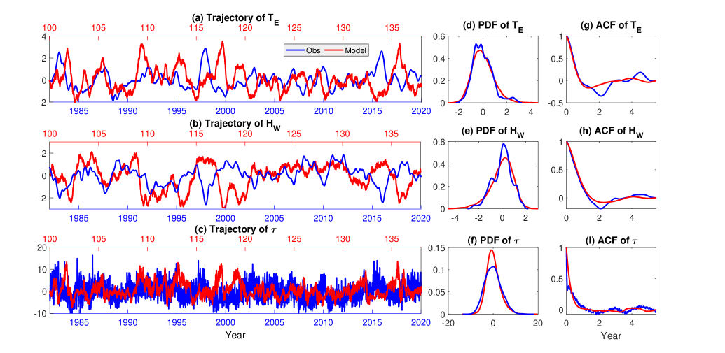
Figure 4: Comparison of the observations (blue) with the simulation from the three-dimensional model (1) with the reference parameters (2) (red). Panels (a)–(c): time series trajectories. Panels (d)–(f): PDFs. Panels (g)–(i): ACFs. Note that Panels (a)–(c) simply show one random realization of the model and thus there is no one-to-one correspondence between the blue and red trajectories (model v.s. observations). The x-axis on the top of each panel is for the model simulation while the one on the bottom is for the observations.

Figure 4 in the Supporting Information shows that the prior model (1) can reproduce the qualitative features of the Niño 3 SST index and the associated non-Gaussian statistics. Yet, as we shall see, the model alone cannot produce effective forecasts or more complex features. Consequently, neural networks trained using the prior data alone will not exhibit the most effective prediction skill (See Section 5.4). This further motivates the development of a BML framework that combines the observational time series with the model simulation to reduce the model error and improve the forecast skill of the Niño 3 index.

4 A Bayesian machine learning (BML) algorithm

We now discuss a Bayesian machine learning (BML) algorithm which takes into account both the prior data described in 3 with the observation data described in 2. Let $\mathbf{v}(t)$ be the prior data, which is a long time series from the prior parametric model (1), and $\mathbf{u}(t)$ be the short observational time series. Here $\mathbf{v}(t)$ and $\mathbf{u}(t)$ can both be one-dimensional, representing the time series of $T_{E}$, or they can be multi-dimensional time series containing any subset of the three variables $T_{E},H_{W}$, and $\tau$.

Denote by $\boldsymbol{\theta}$ the parameters in the neural network and $\boldsymbol{\theta}_{k}$ the estimated parameters after the $k$-th iteration in the stochastic gradient descent (SGD) method Bottou (2010). Next, denote by $\mathbf{x}^{D}_{i}$ and $\mathbf{y}^{D}_{i}$ for $i=1,\ldots,N_{D}$ the input and output data, constructed from the prior time series $\mathbf{v}(t)$, where each $\mathbf{x}^{D}_{i}$ is a delay embedded time series of $\mathbf{v}(t)$ with an appropriate delay embedding time and each $\mathbf{x}^{D}_{i}$ is a corresponding forecast value. Denote by $\mathbf{x}^{O}_{i}$ and $\mathbf{y}^{O}_{i}$ for $i=1,\ldots,N_{O}$ the input and output data constructed from $\mathbf{u}(t)$ in the same way that $\mathbf{x}^{D}_{i}$ and $\mathbf{y}^{D}_{i}$ are constructed from $\mathbf{v}(t)$. Since the observational time series is much shorter than the prior time series, we have $N_{O}\ll N_{D}$. Note that the input and output data will be further specified in Section 5.1.

Define two loss functions $L^{D}$ and $L^{O}$ in training the neural network (NN). The first loss function is exploited to provide a potential update to the parameters $\boldsymbol{\theta}$,

$$L^{D} =\sum_{i}\|\mathbf{y}^{D}_{i}-\mbox{NN}(\mathbf{x}^{D}_{i};\boldsymbol{\theta})\|^{2}$$ (3a)

$$\boldsymbol{\theta}_{k+1}^{D} =\boldsymbol{\theta}_{k}^{D}-\eta^{D}_{k}\left.\frac{\partial L^{D}}{\partial\boldsymbol{\theta}}\right|_{\boldsymbol{\theta}=\boldsymbol{\theta}_{k}^{D}},$$ (3b)

where $\|\cdot\|$ in Eq. (3a) is a given metric for computing the loss function, such as the mean-squared error. We should point out one can always define a computationally reasonable loss function with a metric that is adequate for quantifying the error of the point estimator. The loss function in (3a) corresponds to the standard empirical least-squares regression in supervised learning.

The equation (3b) is the SGD for updating the parameters in the neural network, where $\eta^{D}_{k}$ is the standard learning rate. Note that the observational information is not involved in (3); it only appears in the second loss function,

$$L^{O}=\sum_{i}\|\mathbf{y}^{O}_{i}-\mbox{NN}(\mathbf{x}^{O}_{i};\boldsymbol{\theta})\|^{2},$$ (4)

which is used to validate the proposed parameters formulated in (3b). The BML training algorithm contains two steps in each iteration cycle for updating $\boldsymbol{\theta}$. Denote by $\boldsymbol{\theta}_{k}^{*}$ the current parameter estimate.
Step 1: Proposal. Generate a proposal $\boldsymbol{\theta}^{D}_{k+1}$ as a potential update by utilizing (3b) with $\boldsymbol{\theta}^{D}_{k}=\boldsymbol{\theta}^{*}_{k}$. Note that only the prior information is used in this step.
Step 2: Validation. Evaluate the likelihood function (4) on the proposal $\boldsymbol{\theta}_{k+1}^{D}$ obtained from Step 1. Then the resulting value of the loss function $L^{O}(\boldsymbol{\theta}_{k+1}^{D})$ is compared with $L^{O}(\boldsymbol{\theta}_{k}^{*})$. If the relationship $L^{O}(\boldsymbol{\theta}_{k+1}^{D})\geq L^{O}(\boldsymbol{\theta}_{k}^{*})$, we reject the proposal and repeat Step 1 with $\boldsymbol{\theta}^{*}_{k+1}=\boldsymbol{\theta}^{*}_{k}$. Otherwise, accept the proposal and let $\boldsymbol{\theta}^{*}_{k+1}=\boldsymbol{\theta}^{D}_{k+1}$ and repeat Step 1. If the proposed parameters are rejected in the last $S$ consecutive cycles, which means the proposed parameters fail to improve the loss function (4) (i.e., the likelihood based on the observational data), then the training process will be terminated.

We call this training procedure the Bayesian Machine Learning (BML) algorithm since the two steps above are very similar to those of the Bayesian Markov chain Monte Carlo algorithm. We should point out that the resulting predictor is a point estimator (one neural-network model). Once the model is trained via BML, the prediction of the resulting NN model is no different than the standard ML testing procedure. It is worthwhile to point out that the proposed training algorithm is not similar to the well-known Bayesian Neural Networks (BNN) MacKay (1995), Lampinen and Vehtari (2001) which has widely been used, such as in language modelling and sentiment analysis Gal and Ghahramani (2016), Mukhoti and Gal (2018). The BNN aims to construct a posterior distribution of hyperparameters $\theta$, from which one can employ an ensemble of NN models with $\theta$ sampled from the estimated posterior distribution and subsequently uses the ensemble average as a point estimator or ensemble variance to quantify uncertainties of the point estimator. Technically, BNN requires a specification of the prior distribution of the hyperparameter $\theta$ and employs the optimization on the observed data (so it is not designed to overcome a shortage of observation data).

The BML algorithm is especially useful when only short observations and an approximate parametric model that contains model error are available. Note that the loss function in (4) is not directly used with the SGD to update $\boldsymbol{\theta}$ as would be the case when using the observation datasets to train a neural network. This is because the limited observational data results in large variance and, due to the bias-variance tradeoff Geman et al. (1992), larger expected error, thereby degrading forecast skill. On the other hand, although training with a sufficient amount of prior data results in lower variance and a robust training algorithm, the model error in the prior data may result in biased estimation of $\boldsymbol{\theta}$. The BLM algorithm attempts to de-bias this estimate by accepting/rejecting the proposed network parameters based on the value of the loss function on the observation data.

As a remark, the second step of the above algorithm, namely (4), can also be understood as a special validation procedure Mello and Ponti (2018), El Naqa et al. (2018) in the neural network training process. Since it utilizes only observational data, we call it the “data-driven validation”. As will be seen in Section 5.4, the proposed BLM algorithm outperforms standard neural network training and validation procedures in the case of ENSO forecasting.

5 Results

5.1 Setup

We employ a feedforward net with three hidden layers. The first two hidden layers have $32$ $\tanh$ units each and the final hidden layer has $128$ linear units. The output layer consists of $50$ linear units. The network uses SGD to minimize the root-mean-square error (RMSE) with batch sizes of $128$. In the following experiments, different input data are used, which may contain only a single variable $T_{E}$, two variables $(T_{E},H_{W})$ or three variables $(T_{E},H_{W},\tau)$. Each input, corresponding to an $\mathbf{x}^{D}_{i}$ in Section 4, takes into account a delay embedded time series. Here, the delay embedding time for $T_{E}$ and $H_{W}$ is the past $8$ weeks, and that for $\tau$ is the past $8$ days. Weekly data is used for $T_{E}$ and $H_{W}$ while daily data is used for $\tau$. The output contains only $T_{E}$. The $i$-th output $\mathbf{y}^{D}_{i}$ represents the forecast value of $T_{E}$ at the lead time of the $i$-th week, where $i=1,\ldots,50$. As we stated before, $\{\mathbf{x}^{O}_{i},\mathbf{y}^{O}_{i}\}$ will be constructed in the same way as $\{\mathbf{x}^{D}_{i},\mathbf{y}^{D}_{i}\}$, except that the former consists of only the observed data, $\mathbf{u}(t)$. The parameter $S$ in the BML is set to be $S=20$. This parameter was determined by a quick test on validation data but the authors found that the $S=15$ and $S=25$ yield similar results so the performance of the BML algorithm using the suggested network is not too sensitive to the choice of $S=20$.

In each experiment, the training data is generated by integrating the prior model (1) forward in time until there are approximately $30,000$ weekly samples of $T_{E}$ and $H_{W}$ for training (with daily windburst values chosen appropriately to match current time values of $T_{E}$ and $H_{W}$ during training). This is done by integrating forward on a daily scale and keeping every seventh observation. The efficacy of the learning algorithm is checked using a two-fold test by splitting the observation data into two time periods: first using the 1983-1999 data as training and the 2001-2020 data as testing and then vice-versa. The data in the year 2000 is excluded to prevent the overlap between the training and testing periods. The overall prediction skill is measured by evaluating the normalized RMSE (NRMSE) and pattern correlation (Corr) between the truth and the predicted time series in the entire period (1983–2020 except the year 2000). The Corr and NRMSE are defined as:

$$\begin{split}\mbox{Corr}&=\frac{\sum_{i=1}^{n}(u^{f}_{i}-\bar{u}^{f})(u^{o}_{i}-\bar{u}^{o})}{\sqrt{\sum_{i=1}^{n}(u^{f}_{i}-\bar{u}^{f})^{2}}\sqrt{\sum_{i=1}^{n}(u^{o}_{i}-\bar{u}^{o})^{2}}},\\ \mbox{NRMSE}&=1-\frac{\mbox{RMSE}}{\mbox{std}(u^{o})},\qquad\mbox{where~{}RMSE}=\sqrt{\frac{\sum_{i=1}^{n}(u^{f}_{i}-u^{o}_{i})^{2}}{n}},\end{split}$$ (5)

where $u^{f}_{i}$ and $u^{o}_{i}$ are the forecast and the truth, respectively, at time $t=t_{i}$. The time averages of the forecast and the true time series are denoted by $\bar{u}^{f}$ and $\bar{u}^{o}$ while std$(u)$ is the standard deviation of the truth. The NRMSE starts from NRMSE $=1$ and loses its skill once it reaches the value NRMSE $=0$, at which point the RMSE in the forecasted time series is equal to the standard deviation of the truth. The pattern correlation loses its skill when Corr$<0.5$.

5.2 Forecasts Using Different Inputs

Figure 1 shows the forecast skill of different inputs, using the BML algorithm, and compares them to the classical approach of training the network for a fixed number of epochs.

The skill scores in Panels (a)–(b) indicate that the persistence forecast (purple curves) is skillful only up to $5$ months. The traditional ensemble forecast (green curves) based on the 3D model (1) outperforms the persistence forecast and it remains effective for up to about $6$ months. Yet, this purely model-based ensemble forecast is far less skillful than the BML forecast. Even in the situation with only $T_{E}$ being the input (blue curves), the BML forecast remains skillful for up to nearly $7.5$ months. This indicates the advantage of the machine learning forecast over the traditional ensemble forecast based on parametric models.

Next, if all the three variables $(T_{E},H_{W},\tau)$ are used as the input, then the BML forecast skill can be further extended from $7.5$ to $9.5$ months (red curves). The WWBs are known to be important triggering effects of the El Niño Seiki and Takayabu (2007), Lian et al. (2014), Hu et al. (2014), Thual et al. (2016) and this is reflected in the BML forecast shown here. Specifically, Panels (c)–(d) of Figure 1 indicate that the forecast with the additional input of the wind bursts can capture the timing of the strong El Niño (1987-1988 and 1997-1998) more accurately. It is important to note that since the wind bursts lie in the intraseasonal time scale, only the wind burst data during the past $8$ days is used as the BML input, which is much shorter than the $8$-week input data of $T_{E}$ and $H_{W}$. Such a multiscale feature for the input is crucial in facilitating the effective BML forecast.

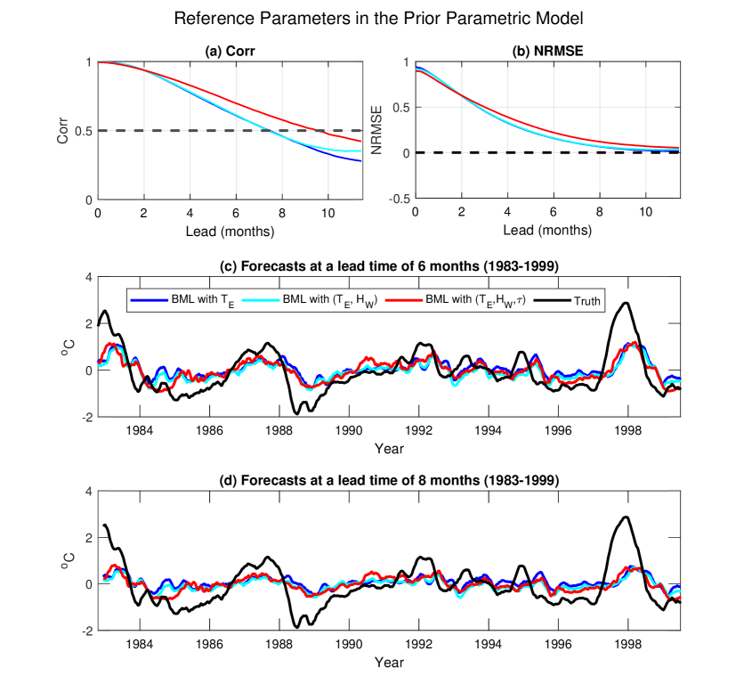
Figure 5: Similar to Figure 1 in the main text, except that the BML forecast using $(T_{E},H_{W})$ as the input (cyan) is included. To clarify the presentation, the persistence and 3D model ensemble forecast have been ignored here.

We also found that the BML forecast with $(T_{E},H_{W})$ as input has about the same skill as the forecast where $T_{E}$ is the only input (see Figure 5 in the Supporting Information). A plausible explanation for this result is as follows. According to the celebrated recharge-discharge theory Jin (1997), the variables $T_{E}$ and $H_{W}$ are the two components of a coupled system that forms an oscillator. Since the input of the BML contains the historic data up to the past $8$ weeks, the information in $H_{W}$ has been characterized by such historic data of $T_{E}$ according to the Takens’ delayed embedding theorem Takens (1981). Thus, including the additional variable $H_{W}$ as the input provides little improvement for the BML forecast. Note that the use of both the current and the past data as the BML input shares a similar mechanism as the delayed oscillator theory Suarez and Schopf (1988), Battisti and Hirst (1989), which involves only a single variable but contains the historical values in the differential equations.

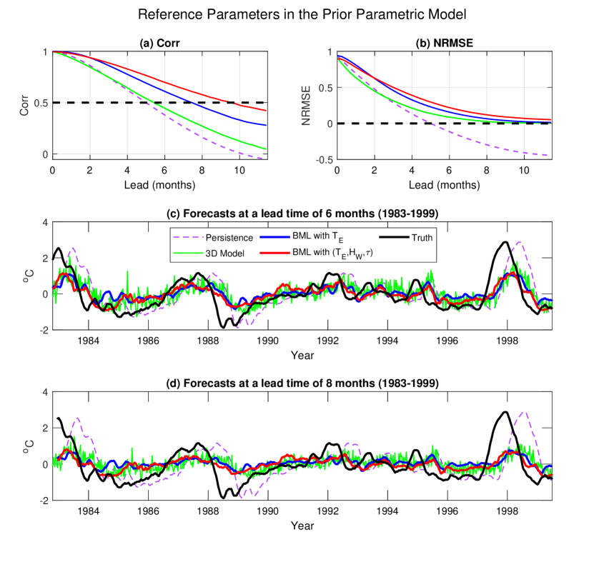
Figure 1: Comparison of the forecasts of different inputs. Panels (a)–(b): skill scores of the persistence forecast (purple), the ensemble forecast using the 3D parametric model (green), the BML forecast using only $T_{E}$ as the input (blue), and the BML forecast using $(T_{E},H_{W},\tau)$ as the input (red). Panels (c)–(d): Comparison of the truth (black) and different forecasts at lead times of $6$ and $8$ months, respectively, during the 1982-1999 period. The predicted time series during the 2001-2020 period is included Figure 6.

5.3 Reducing the Spring Predictability Barrier

Figure 2 shows the forecasts starting from different months. Both the persistence and the ensemble forecast using the 3D model suffer from the so-called spring predictability barrier Duan and Wei (2013), Barnston et al. (2012). In particular, the forecast is quite challenging when starting from February, March, or April, where the skillful forecast only lasts for up to $4$ months. The BML forecast with a single variable $T_{E}$ as the input slightly improves the forecast skill starting from February and March while the useful forecast starting from April is significantly extended to $9$ months. The more improved forecast results are provided by the BML with $(T_{E},H_{W},\tau)$ being the input. In this case, the skillful forecast lasts for nearly $10$ months starting from any time between February to August. In particular, the Corr remains above $0.75$ at a lead time of $4$ months when the starting time is boreal spring and the threshold of Corr $=0.5$ is nearly uniform for different starting months. Since the wind accounts for a large portion of the uncertainty in the ENSO forecast, the improved results here are consistent with the viewpoints in Yu et al. (2009), Mu et al. (2007) that exploited an advanced approach to study different initial uncertainties in affecting the ENSO forecast. Notably, the forecast skill starting from April is significantly improved using the BML. This finding supports the argument in Kirtman et al. (2001), Duan and Wei (2013) that indicates the forecast starting in this season is relatively easy and there is no notable spring predictability barrier phenomenon.

Figure 2: Seasonal prediction: pattern correlation as a function of starting month (y-axis) and lead time (x-axis). Panel (a): persistence. Panel (b): ensemble forecast using the 3D parametric model. Panel (c): the Bayesian machine learning forecast using only $T_{E}$ as the input. Panel (d): Bayesian machine learning forecast using $(T_{E},H_{W},\tau)$ as the input.

5.4 Comparison to Standard Machine Learning training Procedures

Now we report more numerical experiments to get a better sense of the BML algorithm. All the experiments in this subsection employ the variables $(T_{E},H_{W},\tau)$ as the input. Note that the SGD can approach a local minimum of the loss function, which is generally nonconvex, so the initial value of $\boldsymbol{\theta}$ is a source of uncertainty in the neural network training. Another source of the uncertainty comes from the random realizations of the prior time series. To account for these uncertainties, we run the training and forecasting algorithm $10$ times for each experiment with different initial guesses of $\boldsymbol{\theta}$ and different realizations of the prior time series. The shading area in Figure 3 shows the 95% confidence interval of the forecast skill for each experiment.

Figure 3 compares the BML forecast (panel (b)) with the forecast of the same neural network architecture trained in a standard fashion (panel (a)), using (3) for a fixed number of epochs instead of the validation Step 2. The red curve in Panel (a) shows that the neural network trained for a fixed number of epochs on only the prior time series results in a forecast that remains skillful for only $7.5$ month, which is much shorter than the BML forecast ($9.5$ months) shown in Panel (b). Importantly, as is shown by the green curve in Panel (a), in the absence of the data-driven stopping criterion (4), even if the observational and the prior data are both included in (3) for training the network, the resulting forecast skill has little improvement. These findings indicate the importance of using the limited observational data to validate the proposals using (4). On the other hand, as anticipated, when the prior time series is replaced by the short observations in (3) for updating $\boldsymbol{\theta}$, the small amount of training data leads to an extremely unskillful forecast (the yellow curves).

One important issue is to understand the robustness of the proposed scheme to the choice of the validation set in applying the second step of BML. In Panel (c) of Figure 3, it is shown that if the short observations are replaced by a prior time series from a time interval independent from the one used in (3), then the skillful forecast becomes less than $8.5$ months (blue curve). Notably, the confidence interval associated with such an experiment has no overlap with that using the short observations as the validation set (red curve) at the Corr $=0.5$ threshold, which indicates the statistical significance of the difference between these two methods. Another test is to first mix the long prior data and the short observational data, which is then followed by splitting the mixed data into the training and validation sets for Eq. (3) and Eq. (4), respectively. However, since the prior data is much longer than the observations, such an approach (green curve) leads to essentially the same forecast result as the one without the observational data (blue curve). These facts highlight the importance of the data-driven validation (4) that serves as the likelihood function in the BML framework.

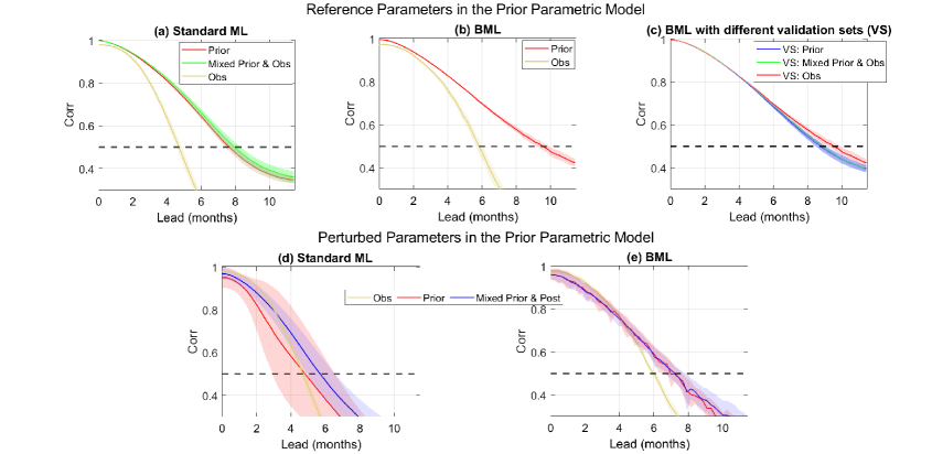
Figure 3: Panels (a)–(c): Comparison of different setups in the machine learning (ML) algorithms. Panel (a): forecasting using the standard ML algorithm. Here, no validation criterion (or step 2 of BML) is used to guide the training in (3). The red and yellow curves indicate the forecasts, in which only the prior data and only the short observations are used for training, respectively. The green curve shows the forecast skill, where the training data is the concatenation of the long prior data and the short observations. Panel (b): forecasting using the BML algorithm. The red curve is the one that is the same as that in Figure 1. It exploits the prior data for the parameter updating (3) in the training process while the short observations are adopted for the data-driven validation (4) as the stopping criterion. The yellow curve uses the short observations for both parameter updating and the data-driven validation. Panel (c): forecasting using the BML algorithm but using different validation sets. The red curve is the same as that in Panel (b). The blue one uses the prior data for validation (4) while the green one uses the mixed prior data and the observations for validation. The shading area shows the uncertainty (95% confidence interval) based on $10$ repeated experiments, which contain different realizations of the prior data. Panels (d)–(e): Comparison of the standard and the BML algorithms in the situation with random perturbed parameters in the prior parametric model. The red and yellow curves indicate the forecasts, in which only the prior data and only the short observations are used for training, respectively. The blue curve shows the forecast, where the training data is the concatenation of the prior and posterior time series. The shading area shows the uncertainty based on $10$ repeated experiments, which contain different realizations of the prior data. In all the panels, the input variables are $(T_{E},H_{W},\tau)$.

5.5 Sensitivity of BML Algorithm Under Perturbations of the Prior Model

The prior time series in all the tests that we have shown so far were generated from the 3D parametric model (1) with the reference parameters (2). While the modeling error prohibits this model to reflect more complex features, such as the spatiotemporal patterns of the ENSO diversity, it qualitatively reproduces the characteristics of the Niño 3 SST time index (as shown in Fig. 4). It is therefore critical to understand the sensitivity of the BML algorithm to the choice of prior models. With this goal in mind, we randomly perturb the reference parameters and check the forecast skills of the standard machine learning and the BML algorithms, when both models are trained using the training data from the perturbed prior models. We repeat the experiments with the perturbed parameters $10$ times. In each experiment, we add random Gaussian noise to each of the reference parameters in (2), where the random Gaussian noise has zero mean and variance $0.8$. The model simulation with the perturbed parameters is illustrated in the Supporting Information.

In Panels (d)–(e) of Figure 3, we show the averaged skill score over the $10$ outcomes for each experiment as well as the associated uncertainty (shading area), which mimic the scenario of the multi-model forecast except that each “model” here is a machine learning forecast, obtained based on training data generated by the prior model with different parameters. Panel (d) shows the results using the standard machine learning forecast algorithm (red curve). Due to the relatively large model error in the prior model, the averaged skill score using the prior time series as the training data is $5$ months, which is only slightly better than the forecast using the short observational data for training (yellow curve). The associated uncertainty (red shading area) using the standard machine learning forecast is also quite large. The forecast results using the standard machine learning algorithm can be improved if the prior time series are concatenated with the so-called posterior time series. These posterior time series are obtained by using a recently developed sampling algorithm Chen (2020), which exploits data assimilation to sample a collection of time series based on the prior model and the short observations. See the Supporting Information for technique details. Using these posterior time series as the training data, the skillful forecast of the standard machine learning algorithm can be extended to about $6$ months together with a reduction of the forecast uncertainty.

In contrast, despite the large model error in the prior model with the perturbed parameters, the forecast skill score using the BML, as is shown in the red curve in Panel (e) of Figure 3, is still skillful up to $7$ months. Also, the uncertainty (red shading area) is significantly smaller than the uncertainty of the standard machine learning forecast, which indicates that the BML algorithm is robust. These merits are due to the data-driven validation (4), which significantly reduces the model error in the prior time series. One interesting finding is that even if one includes posterior time series obtained using a class of data assimilation schemes (See the Supporting Information for details) into the training data for updating $\boldsymbol{\theta}$ of (3) (blue curve in Panel (e)), the skill score remains almost the same as that using only the prior data in (3). This is because the BML algorithm has already taken into account the combined information from the prior model and the observations through the two steps in the training procedure, which captures the information contained in the posterior time series with less uncertainty. This suggests another practical advantage of BML: it does not depend on posterior time series produced by a separate “data assimilation” scheme that may involve non-negligible computational efforts, depending on the complexity of the prior model.

6 Conclusion

In this article, a simple and efficient BML training algorithm, which exploits only short observational time series and an approximate parametric model, is developed to provide effective predictions of the Niño 3 SST index. The BML forecast significantly outperforms the model-based ensemble predictions and standard machine learning forecasts. It also overcomes the spring predictability barrier to a large extent. The BML algorithm allows a multiscale input consisting of both the SST and the wind bursts, which improved prediction skills over the forecasts where SST is the sole variable. Finally, the BML algorithm also reduces the forecast uncertainty and produces robust results even when the training data is generated by prior models that are significantly perturbed from its reference parameter.

The primary goal here is to provide a new and efficient training framework that facilitates a predictive machine learning model even when there is a small amount of available training data. The main idea is to supplement the training strategy with a set of computer-generated data from a model to reduce the large variance error usually present in an ML model trained using a standard training procedure. While the BML may not be better than the standard training procedure when a large dataset becomes available, it is worthwhile to try and determine the length of observational data required so that the two methods are comparable. This is a complicated study to undertake since it may depend on the class of neural network models and the choice of prior models. Unfortunately, in the context of SST prediction, such a study may not be conclusive due to the shortage of available data and unknown underlying dynamics. We plan to address this issue in a more controlled environment, where the underlying dynamics are known. Finally, while the framework is rather simple and can be used in any application where there are a small number of observations, the effectiveness of the method depends on the choice of prior model. In real applications, since the underlying dynamical model is not available, the main task is to identify an effective prior model. In the context of SST prediction with time series training data, we have shown the effectiveness of BML over standard training procedure using the SDE in (1) as prior. For future work, we plan to inspect whether other variables, such as the tropical and extratropical precursors Chen et al. (2020), Boschat et al. (2013) can improve the SST forecast. It is also interesting to use operational models as the prior to test the BML algorithm. Another natural future work using the new Bayesian machine learning framework is to skillfully forecast spatiotemporal patterns of the ENSO diversity.

Supporting Information for “A Bayesian Machine Learning Algorithm for Predicting ENSO Using Short Observational Time Series”

Contents of this file

1. Comparison of the Simulation from the 3D Model with the Observations

2. More Results of the BML Forecasts with the reference Parameters in the Prior Model

   1. BML Forecasts Using Different Inputs

   2. Forecasts Using Different Inputs

3. Details of the BML Forecasts with Perturbed Parameters in the Prior Model

   1. The Model with Perturbed Parameters

   2. Discussion of the Conditional Sampling Method that Generates the Posterior Time Series

Additional Supporting Information (Files uploaded separately)

1. Source code for the BML training and forecasts.

1 Comparison of the Simulation from the 3D Model with the Observations

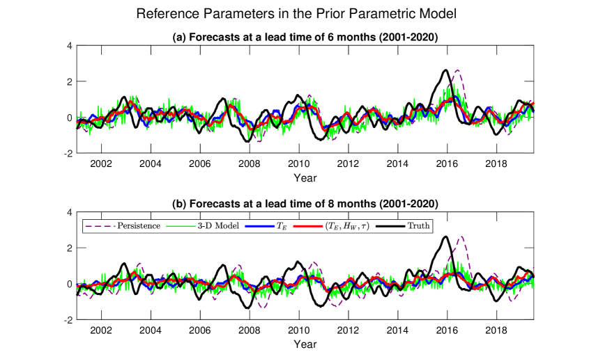
Figure 6: Similar to Panels (c)–(d) of Figure 1 in the main text, except the results are in the 2001-2020 time period.

Panels (a)–(c) of Figure 4 show a comparison between the model trajectories and the observational time series. Here the reference parameters (2) are used in the model (1). The results here indicate qualitatively consistent path-wise behavior. Panels (d)–(i) compare the PDFs and the ACFs, and show that the observed non-Gaussian statistics of all of the three variables are reproduced by the model to a large extent. As seen Figures 1 and 6, this model can reproduce the climatological statistics and trajectories that qualitatively reflect the time scale of the truth; but, its predictive skill is less effective than the proposed BML algorithm due to the model error.

2 More Results of the BML Forecasts with the Reference Parameters in the Prior Model

2.1 BML Forecasts Using Different Inputs

Figure 5 shows the BML forecast using different inputs. It is similar to Figure 1 in the main text, except that the BML forecast using $(T_{E},H_{W})$ as the input (cyan) is also included. The results here show that the forecast with input $(T_{E},H_{W})$ is similar to the one with $T_{E}$ as the only input.

2.2 Forecasts Using Different Inputs

Figure 6, which is similar to Panels (c)–(d) of Figure 1 in the main text, shows the forecasts obtained from different inputs. The only difference is that the results in Figure 6 are in the 2001-2020 period.

3 Details of the BML Forecasts with Perturbed Parameters in the Prior Model

3.1 The Model with Perturbed Parameters

We still adopt the same model as in (1) when considering the model error case, But we add independent Gaussian random noise with mean $0$ and variance $.8$ to each parameter. Figure 7 show $5$ perturbed models with different random parameters (red curves) along with the observations (blue curves). For simplicity, the random number seeds are fixed here. Therefore, the main difference in these perturbed parameter cases is the amplitude, phase and noise levels in the time series. It is clear that some imperfect models (e.g., Cases #2 and #3) are qualitatively reasonable while some other perturbed models (e.g., Cases #4 and #5) are quite different from the observations. This situation mimics the multi-model forecast scenario, where the differences between the models can be quite dramatic.

3.2 Discussion of the Conditional Sampling Method that Generates the Posterior Time Series

In this section, we briefly discuss the conditional sampling method that generates the posterior time series that are used in assessing the robustness of BML (see blue curves in panels (c)-(d) in Figure 3. In particular, we will sample the following conditional distribution,

$$p(\mathbf{v}(t)|\mathbf{u}([0,T])),\quad 0\leq t\leq T,$$

where $\mathbf{v}(t)$ and $\mathbf{u}([0,T])$ are the time series of the prior model and the observations,respectively on the training time interval $[0,T]$. Numerically, we sample the above conditional distribution by solving a system of stochastic differential equations resulting from a nonlinear version of the Kalman smoother applied to the prior model in (1). The mathematical details are shown in (Chen, 2020). Therefore, the sampled trajectories have the same length as the observations and they lie in the same time interval. In a nutshell, we effectively leverage the randomness in the prior model (1), reflected by the stochastic noises, to generate multiple trajectories that contain the information from both the observations and the prior model.

In the model with reference parameters, the sampled trajectories highly resemble the observations. See Panels (a)–(b) in Figure 8.

In the situation with perturbed parameters, we focus on Case #1 shown in Figure 7. The perturbed parameters are $\alpha_{1}=2.2603$, $\alpha_{2}=.8676$, $d_{\tau}=4.1833$, $d_{T}=d_{H}=2.1393$, $\omega_{u}=-1.3890$, $\sigma_{T}=\sigma_{H}=2.1324$. Furthermore, the original $\sigma_{\tau}$ parameter is multiplied by $0.6715$. As shown in the first row of Figure 7 (red color), the prior time series generated from the perturbed model exhibits It can be seen from panel (b) of Figure 8, that the sampled trajectories have less error than the prior time series. This is the fundamental reason that the traditional neural network forecast skill can be improved when the prior and posterior time series are used together for training (Panel (d) of Figure 3). Note that the length of the posterior time series is the same as the length of the short time observations. Therefore, although the multiple posterior time series plays an important role in reducing the bias (model error) in the training data when compared with the training based only on the prior time series, these short posterior time series may not cover the entire solution space associated with the true underlying dynamics. The prior time series can be included in the training dataset to expand the solution space, thereby compensating for this shortcoming of the posterior time series.

It is worthwhile to point out that in the simulation above, since the prior model in (1) has a special structure (it is conditionally Gaussian), the resulting smoothing equation can be realized analytically (Chen, 2020). Unfortunately, such structure is not amenable to generalization, and applying the conditional sampling algorithm for general nonlinear systems in high dimensional space requires additional computational efforts that can be expensive. For example, when ensemble Kalman smoother is used, the number of the ensemble members must be increased (exponentially) in the Bayesian update step to retain accurate numerical solutions. Our numerical results (compare the blue and red curves in panel (e) of Figure. 3) suggest that the proposed BML algorithm can readily account for the information in the posterior time series without having to realize it with an additional smoother algorithm, and thus, additional computational cost can be avoided.

Figure 7: The model (1) with perturbed parameters. The five rows show five groups of perturbed parameters. The three columns compare the time series, PDFs and ACFs with the truth.

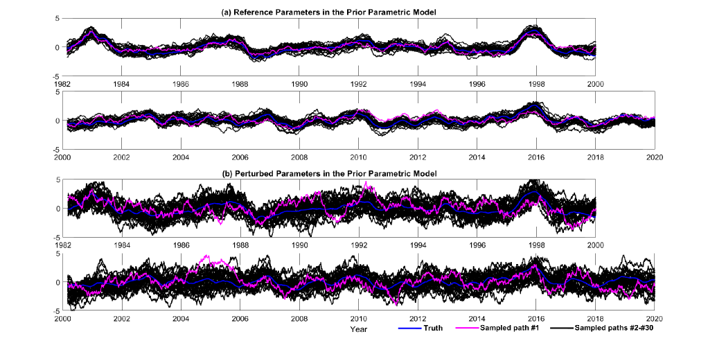
Figure 8: Comparison of the observed SST (blue) and the 30 sampled of posterior time series (magenta and black). One sampled trajectory is marked by magenta color for the convenience of comparing with the observation. Panel (a): sampled trajectories using the smoothing equation corresponding to the prior model (1) equipped with the reference parameter. Panel (b): Same as (a) except that the prior model is perturbed. Here, we show sampled trajectories corresponding to Case #1 in Figure 7.

References

- Ashok and Yamagata (2009) K. Ashok and T. Yamagata. The El Niño with a difference. Nature, 461(7263):481–484, 2009.
- Barnston et al. (2012) A. G. Barnston, M. K. Tippett, M. L. L’Heureux, S. Li, and D. G. DeWitt. Skill of real-time seasonal ENSO model predictions during 2002–11: Is our capability increasing? Bulletin of the American Meteorological Society, 93(5):631–651, 2012.
- Barrett et al. (2018) H. G. Barrett, J. M. Jones, and G. R. Bigg. Reconstructing El Niño Southern Oscillation using data from ships’ logbooks, 1815–1854. Part I: methodology and evaluation. Climate dynamics, 50(3):845–862, 2018.
- Battisti and Hirst (1989) D. S. Battisti and A. C. Hirst. Interannual variability in a tropical atmosphere–ocean model: Influence of the basic state, ocean geometry and nonlinearity. Journal of Atmospheric Sciences, 46(12):1687–1712, 1989.
- Behringer et al. (1998) D. W. Behringer, M. Ji, and A. Leetmaa. An improved coupled model for ENSO prediction and implications for ocean initialization. Part I: The ocean data assimilation system. Monthly Weather Review, 126(4):1013–1021, 1998.
- Bernardo and Smith (2009) J. M. Bernardo and A. F. Smith. Bayesian theory, volume 405. John Wiley & Sons, 2009.
- Boschat et al. (2013) G. Boschat, P. Terray, and S. Masson. Extratropical forcing of ENSO. Geophysical Research Letters, 40(8):1605–1611, 2013.
- Bottou (2010) L. Bottou. Large-scale machine learning with stochastic gradient descent. In Proceedings of COMPSTAT’2010, pages 177–186. Springer, 2010.
- Box and Tiao (2011) G. E. Box and G. C. Tiao. Bayesian inference in statistical analysis, volume 40. John Wiley & Sons, 2011.
- Chen et al. (2020) H.-C. Chen, Y.-H. Tseng, Z.-Z. Hu, and R. Ding. Enhancing the ENSO predictability beyond the spring barrier. Scientific reports, 10(1):1–12, 2020.
- Chen (2020) N. Chen. Can short and partial observations reduce model error and facilitate machine learning prediction? Entropy, 22(10):1075, 2020.
- Clarke (2008) A. J. Clarke. An Introduction to the Dynamics of El Niño and the Southern Oscillation. Elsevier, 2008.
- Di Lorenzo et al. (2010) E. Di Lorenzo, K. Cobb, J. Furtado, N. Schneider, B. Anderson, A. Bracco, M. Alexander, and D. Vimont. Central pacific El Nino and decadal climate change in the North Pacific ocean. Nature Geoscience, 3(11):762–765, 2010.
- Ding et al. (2018) H. Ding, M. Newman, M. A. Alexander, and A. T. Wittenberg. Skillful climate forecasts of the tropical Indo-Pacific ocean using model-analogs. Journal of Climate, 31(14):5437–5459, 2018.
- Duan and Wei (2013) W. Duan and C. Wei. The ‘spring predictability barrier’ for ENSO predictions and its possible mechanism: results from a fully coupled model. International Journal of Climatology, 33(5):1280–1292, 2013.
- El Naqa et al. (2018) I. El Naqa, D. Ruan, G. Valdes, A. Dekker, T. McNutt, Y. Ge, Q. J. Wu, J. H. Oh, M. Thor, W. Smith, et al. Machine learning and modeling: Data, validation, communication challenges. Medical physics, 45(10):e834–e840, 2018.
- Emile-Geay et al. (2013) J. Emile-Geay, K. M. Cobb, M. E. Mann, and A. T. Wittenberg. Estimating central equatorial Pacific SST variability over the past millennium. Part I: Methodology and validation. Journal of Climate, 26(7):2302–2328, 2013.
- Fine (2006) T. L. Fine. Feedforward neural network methodology. Springer Science & Business Media, 2006.
- Gal and Ghahramani (2016) Y. Gal and Z. Ghahramani. A theoretically grounded application of dropout in recurrent neural networks. Advances in neural information processing systems, 29:1019–1027, 2016.
- Geman et al. (1992) S. Geman, E. Bienenstock, and R. Doursat. Neural networks and the bias/variance dilemma. Neural computation, 4(1):1–58, 1992.
- Gergis and Fowler (2009) J. L. Gergis and A. M. Fowler. A history of ENSO events since AD 1525: implications for future climate change. Climatic Change, 92(3):343–387, 2009.
- Ham et al. (2019) Y.-G. Ham, J.-H. Kim, and J.-J. Luo. Deep learning for multi-year ENSO forecasts. Nature, 573(7775):568–572, 2019.
- Hendon et al. (2007) H. H. Hendon, M. C. Wheeler, and C. Zhang. Seasonal dependence of the MJO–ENSO relationship. Journal of Climate, 20(3):531–543, 2007.
- Hu et al. (2014) S. Hu, A. V. Fedorov, M. Lengaigne, and E. Guilyardi. The impact of westerly wind bursts on the diversity and predictability of El Niño events: An ocean energetics perspective. Geophysical research letters, 41(13):4654–4663, 2014.
- Jin (1997) F.-F. Jin. An equatorial ocean recharge paradigm for ENSO. Part I: Conceptual model. Journal of the atmospheric sciences, 54(7):811–829, 1997.
- Kalnay (2003) E. Kalnay. Atmospheric modeling, data assimilation and predictability. Cambridge university press, 2003.
- Kalnay et al. (1996) E. Kalnay, M. Kanamitsu, R. Kistler, W. Collins, D. Deaven, L. Gandin, M. Iredell, S. Saha, G. White, J. Woollen, et al. The NCEP/NCAR 40-year reanalysis project. Bulletin of the American meteorological Society, 77(3):437–472, 1996.
- Kirtman et al. (2001) B. Kirtman, J. Shukla, M. Balmaseda, N. Graham, C. Penland, Y. Xue, and S. Zebiak. Current status of enso forecast skill: A report to the clivar working group on seasonal to interannual prediction. 2001.
- Kirtman and Min (2009) B. P. Kirtman and D. Min. Multimodel ensemble ENSO prediction with CCSM and CFS. Monthly Weather Review, 137(9):2908–2930, 2009.
- Lampinen and Vehtari (2001) J. Lampinen and A. Vehtari. Bayesian approach for neural networks—review and case studies. Neural networks, 14(3):257–274, 2001.
- LeCun et al. (2015) Y. LeCun, Y. Bengio, and G. Hinton. Deep learning. nature, 521(7553):436–444, 2015.
- Lian et al. (2014) T. Lian, D. Chen, Y. Tang, and Q. Wu. Effects of westerly wind bursts on El Niño: A new perspective. Geophysical Research Letters, 41(10):3522–3527, 2014.
- MacKay (1995) D. J. MacKay. Probable networks and plausible predictions—a review of practical bayesian methods for supervised neural networks. Network: computation in neural systems, 6(3):469–505, 1995.
- Majda and Chen (2018) A. J. Majda and N. Chen. Model error, information barriers, state estimation and prediction in complex multiscale systems. Entropy, 20(9):644, 2018.
- McGregor et al. (2010) S. McGregor, A. Timmermann, and O. Timm. A unified proxy for ENSO and PDO variability since 1650. Climate of the Past, 6(1):1–17, 2010.
- Mello and Ponti (2018) R. F. Mello and M. A. Ponti. Machine learning: a practical approach on the statistical learning theory. Springer, 2018.
- Moore and Kleeman (1998) A. Moore and R. Kleeman. Skill assessment for ENSO using ensemble prediction. Quarterly Journal of the Royal Meteorological Society, 124(546):557–584, 1998.
- Mu et al. (2007) M. Mu, H. Xu, and W. Duan. A kind of initial errors related to ‘spring predictability barrier for el niño events in zebiak-cane model. Geophysical Research Letters, 34(3), 2007.
- Mukhoti and Gal (2018) J. Mukhoti and Y. Gal. Evaluating bayesian deep learning methods for semantic segmentation. arXiv preprint arXiv:1811.12709, 2018.
- Palmer (2001) T. N. Palmer. A nonlinear dynamical perspective on model error: A proposal for non-local stochastic-dynamic parametrization in weather and climate prediction models. Quarterly Journal of the Royal Meteorological Society, 127(572):279–304, 2001.
- Puy et al. (2016) M. Puy, J. Vialard, M. Lengaigne, and E. Guilyardi. Modulation of equatorial Pacific westerly/easterly wind events by the Madden–Julian oscillation and convectively-coupled Rossby waves. Climate dynamics, 46(7-8):2155–2178, 2016.
- Rasmusson and Carpenter (1982) E. M. Rasmusson and T. H. Carpenter. Variations in tropical sea surface temperature and surface wind fields associated with the Southern Oscillation/El Niño. Monthly Weather Review, 110(5):354–384, 1982.
- Rayner et al. (2003) N. Rayner, D. E. Parker, E. Horton, C. K. Folland, L. V. Alexander, D. Rowell, E. Kent, and A. Kaplan. Global analyses of sea surface temperature, sea ice, and night marine air temperature since the late nineteenth century. Journal of Geophysical Research: Atmospheres, 108(D14), 2003.
- Reynolds et al. (2007) R. W. Reynolds, T. M. Smith, C. Liu, D. B. Chelton, K. S. Casey, and M. G. Schlax. Daily high-resolution-blended analyses for sea surface temperature. Journal of climate, 20(22):5473–5496, 2007.
- Ropelewski and Halpert (1987) C. F. Ropelewski and M. S. Halpert. Global and regional scale precipitation patterns associated with the El Niño/Southern Oscillation. Monthly weather review, 115(8):1606–1626, 1987.
- Seiki and Takayabu (2007) A. Seiki and Y. N. Takayabu. Westerly wind bursts and their relationship with intraseasonal variations and ENSO. Part I: Statistics. Monthly Weather Review, 135(10):3325–3345, 2007.
- Suarez and Schopf (1988) M. J. Suarez and P. S. Schopf. A delayed action oscillator for ENSO. Journal of Atmospheric Sciences, 45(21):3283–3287, 1988.
- Takens (1981) F. Takens. Detecting strange attractors in turbulence. In Dynamical systems and turbulence, Warwick 1980, pages 366–381. Springer, 1981.
- Tang et al. (2018) Y. Tang, R.-H. Zhang, T. Liu, W. Duan, D. Yang, F. Zheng, H. Ren, T. Lian, C. Gao, D. Chen, et al. Progress in ENSO prediction and predictability study. National Science Review, 5(6):826–839, 2018.
- Thual et al. (2016) S. Thual, A. J. Majda, N. Chen, and S. N. Stechmann. Simple stochastic model for El Niño with westerly wind bursts. Proceedings of the National Academy of Sciences, 113(37):10245–10250, 2016.
- Tziperman and Yu (2007) E. Tziperman and L. Yu. Quantifying the dependence of westerly wind bursts on the large-scale tropical Pacific SST. Journal of climate, 20(12):2760–2768, 2007.
- Wang et al. (2020) X. Wang, J. Slawinska, and D. Giannakis. Extended-range statistical ENSO prediction through operator-theoretic techniques for nonlinear dynamics. Scientific reports, 10(1):1–15, 2020.
- Watson et al. (2017) P. A. Watson, J. Berner, S. Corti, P. Davini, J. von Hardenberg, C. Sanchez, A. Weisheimer, and T. N. Palmer. The impact of stochastic physics on tropical rainfall variability in global climate models on daily to weekly time scales. Journal of Geophysical Research: Atmospheres, 122(11):5738–5762, 2017.
- Wyrtki (1975) K. Wyrtki. El Niño–the dynamic response of the equatorial Pacific ocean to atmospheric forcing. Journal of Physical Oceanography, 5(4):572–584, 1975.
- Yeh et al. (2009) S.-W. Yeh, J.-S. Kug, B. Dewitte, M.-H. Kwon, B. P. Kirtman, and F.-F. Jin. El Niño in a changing climate. Nature, 461(7263):511–514, 2009.
- Yu et al. (2009) Y. Yu, W. Duan, H. Xu, and M. Mu. Dynamics of nonlinear error growth and season-dependent predictability of el niño events in the zebiak–cane model. Quarterly Journal of the Royal Meteorological Society: A journal of the atmospheric sciences, applied meteorology and physical oceanography, 135(645):2146–2160, 2009.
- Zebiak and Cane (1987) S. E. Zebiak and M. A. Cane. A model El Niño–Southern Oscillation. Monthly Weather Review, 115(10):2262–2278, 1987.