Tighter bounds on transient moments of stochastic chemical systems

Abstract

The use of approximate solution techniques for the Chemical Master Equation is a common practice for the analysis of stochastic chemical systems. Despite their widespread use, however, many such techniques rely on unverifiable assumptions and only a few provide mechanisms to control the approximation error quantitatively. Addressing this gap, Dowdy and Barton [The Journal of Chemical Physics, 149(7), 074103 (2018)] proposed a method for the computation of guaranteed bounds on the moment trajectories associated with stochastic chemical systems described by the Chemical Master Equation, thereby providing a general framework for error quantification. Here, we present an extension of this method. The key contribution is a new hierarchy of convex necessary moment conditions crucially reflecting the temporal causality and other regularity conditions that are inherent to the moment trajectories associated with stochastic processes described by the Chemical Master Equation. Analogous to the original method, these conditions generate a hierarchy of semidefinite programs that furnishes monotonically improving bounds on the trajectories of the moments and related statistics. Compared to its predecessor, the presented hierarchy produces bounds that are at least as tight and it often enables the computation of dramatically tighter bounds as it enjoys superior scaling properties and the arising semidefinite programs are highly structured. We analyze the properties of the presented hierarchy in detail, discuss some aspects of its practical implementation and demonstrate its merits with several examples.

I Tighter Bounds on the Transient Moments of Stochastic Chemical Systems

I.1 Introduction

The analysis of systems undergoing chemical reactions lies at the heart of many scientific and engineering activities. While deterministic models have proved adequate for the analysis of systems at the macroscopic scale, they often fall short for meso- and microscopic systems; in particular for those that feature low molecular counts. In this regime, the complex and chaotic motion of molecules reacting upon collision causes effectively stochastic fluctuations of the molecular counts that are large compared to the mean and, as a consequence, can have a profound effect on the system’s characteristics – a situation frequently encountered in cellular biology Arkin, Ross, and McAdams (1998); Elowitz et al. (2002); Liu and Jia (2004); Artyomov et al. (2007). In the context of the continuously growing capabilities of synthetic biology, this fact motivates the use of stochastic models for the identification, design and control of biochemical reaction networks. However, while in these applications stochastic models provide the essential fidelity relative to their deterministic counterparts, their analysis is generally more involved.

Stochastic chemical systems are canonically modeled as jump processes. Specifically, the system state, as encoded by the molecular counts of the individual chemical species, is modeled to change only discretely in response to reaction events as triggered by the arrivals of Poisson processes whose rates depend on the underlying reaction mechanism. The so-called Chemical Master Equation (CME) describes how the probability distribution of the state of such a process evolves over time. To that end, the CME tracks the probability to observe the system in any reachable state over time. This introduces a major challenge for the analysis of stochastic chemical systems which routinely feature millions or even infinitely many reachable states, rendering a direct solution of the CME intractable. As a consequence, sampling techniques such as Gillespie’s Stochastic Simulation Algorithm Gillespie (1976, 1977) have become the most prominent approach for the analysis of systems described by the CME. Although these techniques perform remarkably well across a wide range of problems, they are inadequate in certain settings. Most notably, they do not scale well for stiff systems, generally do not provide hard error bounds and the evaluation of sensitivity information is challenging Gillespie, Hellander, and Petzold (2013). Specifically, the two latter shortcomings limit their utility in the context of identification, design and control. Alternatives such as the finite state projection algorithm Munsky and Khammash (2006) come with guaranteed error bounds and straightforward sensitivity evaluation, however, suffer generally more severely from high dimensionality.

From a practical perspective, stochastic reaction networks are often sufficiently characterized by only a few low-order moments of the associated distribution of the state, for example through means and variances. In that case, tractability of the CME may be recovered by solving for the moments of its solution directly. The dynamics of a finite sequence of moments associated with the distribution described by the CME, however, do not generally form a closed, square system, hence do not admit a solution by simple numerical integration. Numerous moment closure approximations Ale, Kirk, and Stumpf (2013); Keeling (2000); Nåsell (2003); Smadbeck and Kaznessis (2013) have been proposed to remedy this problem. A major shortcoming of moment closure approximations, however, is that they generally rely on unverifiable assumptions about the underlying distribution and therefore introduce an uncontrolled error. In fact, it is well-known that their application can lead to unphysical results such as spurious oscillations and negative mean molecular counts Schnoerr, Sanguinetti, and Grima (2015, 2014); Grima (2012). Addressing this shortcoming, several authors have recently proposed methods for the computation of rigorous, theoretically guaranteed bounds for the moments (or related statistics) associated with stochastic reaction networks; such bounding schemes have been proposed for the steady Dowdy and Barton (2018a); Ghusinga et al. (2017); Kuntz et al. (2019); Sakurai and Hori (2017) and transient setting Dowdy and Barton (2018b); Sakurai and Hori (2019); Del Vecchio, Dy, and Qian (2016); Backenköhler, Bortolussi, and Wolf (2019), and their utility for the design of biochemical systems has been demonstrated Sakurai and Hori (2018). The key insight underpinning these methods, rooted in real algebraic geometry, is that the moment sequence associated with the true solution of the CME must satisfy a rich set of algebraic conditions reflecting the support and dynamics of the true distribution. Crucially, these conditions only depend on the problem data but do not require explicit knowledge of the true solution. The use of mathematical programming to identify a truncated moment sequence which minimizes (maximizes) a given moment or related statistic of interest subject to these conditions then furnishes a valid lower (upper) bound on the true value. While such bounds provide a mechanism to quantify errors or verify the consistency of approximation techniques, they are even frequently found to be sufficiently tight to be used directly as a proxy for the true solutionSakurai and Hori (2017); Ghusinga et al. (2017); Dowdy and Barton (2018a); Kuntz et al. (2019).

In this work, we extend the bounding scheme proposed by Dowdy and Barton (2018b) for transient moments of the solutions of the CME. To that end, we introduce new necessary moment conditions that improve the tightness of the semidefinite relaxations on which Dowdy and Barton’s approach is based. These necessary moment conditions reflect crucially the temporal causality that is inherent to solutions of the CME. The conditions lend themselves to be organized in a hierarchy that provides a mechanism to trade-off computational cost for higher-quality bounds. Moreover, we show that the conditions exhibit favorable scaling properties and structure when compared to the conditions employed in the original method.

This article is organized as follows. In Section II, we introduce definitions and assumptions, formally define the moment bounding problem, and review essential preliminaries. Section III is devoted to the development and analysis of the proposed hierarchy of necessary moment conditions. In Section IV, we discuss certain aspects pertaining to the use of these conditions for computation of moment bounds in practice. The potential of the developed methodology is demonstrated with several examples in Sections V and VI before we conclude with some open questions in Section VII.

II Preliminaries

II.1 Notation

We denote scalars with lowercase symbols without emphasis while vectors and matrices are denoted by bold lower- and uppercase symbols, respectively. Throughout, vectors are assumed to be column vectors. Generic sets are denoted by uppercase symbols without emphasis. For special or commonly used sets we use the standard notation. For example, for the (non-negative) $n$-dimensional reals and integers, we use the usual notation of $\mathbb{R}^{n}$ ($\mathbb{R}^{n}_{+}$) and $\mathbb{Z}^{n}$ ($\mathbb{Z}^{n}_{+}$), respectively. Similarly, we refer to the set of symmetric and symmetric positive semidefinite (psd) $n$-by-$n$ matrices with $\mathbb{S}^{n}$ and $\mathbb{S}^{n}_{+}$, respectively, and use the usual shorthand notation $\bm{A}\succeq\bm{B}$ for $\bm{A}-\bm{B}\in\mathbb{S}_{+}^{n}$. The set of $n$-dimensional vector and symmetric matrix polynomials with real coefficients (of degree at most $k$) in the variables $\bm{x}=[x_{1}\ \dots\ x_{N}]^{\top}$ will be denoted by $\mathbb{R}^{n}[\bm{x}]$ ($\mathbb{R}^{n}_{k}[\bm{x}]$) and $\mathbb{S}^{n}[\bm{x}]$ ($\mathbb{S}^{n}_{k}[\bm{x}]$), respectively. In order to concisely denote multivariate monomials, we employ the multi-index notation: for a monomial in $n$ variables corresponding to the multi-index $\bm{j}=[j_{1}\,\dots\,j_{n}]^{\top}\in\mathbb{Z}_{+}^{n}$, we write $\bm{x}^{\bm{j}}=\prod_{i=1}^{n}x_{i}^{j_{i}}$. The indicator function of a set $A$ is denoted by $\mathds{1}_{A}$. Lastly, we denote the set of $n$ times continuously differentiable functions on an interval $I\subset\mathbb{R}$ by $\mathcal{C}^{n}(I)$ while the set of absolutely continuous functions will be denoted by $\mathcal{AC}(I)$. The remaining symbols will be defined as they are introduced.

II.2 Problem Statement, Definitions & Assumptions

We consider a chemical system featuring $n$ chemical species $S_{1},\dots,S_{n}$ undergoing $n_{R}$ different reactions. The system state $\bm{x}$ is encoded by the molecular counts of the individual species, i.e., $\bm{x}=[x_{1}\,\dots\,x_{n}]^{\top}\in\mathbb{Z}^{n}_{+}$. It changes in response to reaction events according to the stoichiometry:

$$\nu^{-}_{1,r}S_{1}+\cdots+\nu^{-}_{n,r}S_{N}\rightarrow\nu^{+}_{1,r}S_{1}+\cdots+\nu^{+}_{n,r}S_{n},\quad r=1,\dots,n_{R}.$$

Thus, the system state changes by $\bm{\nu}_{r}=[\nu_{1,r}^{+}-\nu_{1,r}^{-}\ \dots\ \nu_{n,r}^{+}-\nu_{n,r}^{-}]^{\top}\in\mathbb{Z}^{n}$ in response to reaction $r$. We will restrict ourselves to the framework of stochastic chemical kinetics for modeling such systems.

The notion of stochastic chemical kinetics treats the position and velocities of all molecules in the system as random variables; reactions are assumed to occur at collisions with a prescribed probability. Consequently, the evolution of the system state is a continuous-time jump process. Here, we will assume that this jump process can be described by the Chemical Master Equation (CME).

Assumption 1.

Let $P_{\pi}(\bm{x},t)$ be the probability to observe the system in state $\bm{x}$ at time $t$ given the distribution $\pi$ of the initial state of the system. Then, $P_{\pi}(\bm{x},t)$ satisfies

$$\frac{\partial P_{\pi}}{\partial t}(\bm{x},t)=\sum_{r=1}^{n_{R}}a_{r}(\bm{x}-\bm{\nu}_{r})P_{\pi}(\bm{x}-\bm{\nu}_{r},t)-a_{r}(\bm{x})P_{\pi}(\bm{x},t),\\ P_{\pi}(\cdot,0)=\pi$$ (1)

where $a_{r}$ denotes the propensity of reaction $r$, i.e., in state $\bm{x}$, $a_{r}(\bm{x})dt$ quantifies the probability that reaction $r$ occurs in $[t,t+dt)$ as $dt\rightarrow 0$.

Moreover, we will restrict our considerations to the case of polynomial reaction propensities.

Assumption 2.

The reaction propensities $a_{r}$ in (1) are polynomials.

To ensure the moment trajectories remain well-defined at all times, we will further assume that the stochastic process is well-behaved in the following sense.

Assumption 3.

The number of reaction events occurring in the system within finite time is finite with probability 1.

A consequence of Assumption 3 is that the continuous-time jump processes associated with (1) is regular Resnick (1992), i.e., it does not explode in finite time. We wish to emphasize that Assumptions 1 – 3 are rather weak; Assumptions 1 and 2 are in line with widely accepted microscopic models Gillespie (1992) while Assumption 3 should intuitively be satisfied for any practically relevant system for which the CME is a reasonable modeling approach. Furthermore, Assumption 3 is formally necessary for (1) to be valid on $\mathbb{R}_{+}$ Resnick (1992). For a detailed, physically motivated derivation of the CME alongside discussion of the underlying assumptions and potential relaxations thereof, the interested reader is referred to Gillespie (1992).

Instead of studying the probability distribution $P_{\pi}$ as a description of the system behavior, in this paper we will focus on its moments defined as follows.

Definition 1.

Let $X$ be the reachable set of the system, i.e., $X=\{\bm{x}\in\mathbb{Z}_{+}^{n}\mid\exists t\geq 0:P_{\pi}(\bm{x},t)>0\}$, and $\bm{j}\in\mathbb{Z}_{+}^{n}$ be a multi-index. The $\bm{j}$^th moment of $P_{\pi}(\cdot,t)$ is defined as $y_{\bm{j}}(t)=\sum_{x\in X}\bm{x}^{\bm{j}}P_{\pi}(\bm{x},t)$. $y_{\bm{j}}$ is said to be of order $|\bm{j}|=\sum_{i=1}^{n}j_{i}$. The function $y_{\bm{j}}(\cdot)$ is called the trajectory of the $\bm{j}$^th moment.

Additionally, it will prove useful to introduce the following notion of generalized moments.

Definition 2.

Let $y_{\bm{j}}$ be as in Definition 1 and $t_{T}>0$. Consider a uniformly bounded Lebesgue integrable function $g:[0,t_{T}]\rightarrow\mathbb{R}$. The $\bm{j}$^th generalized moment of $P_{\pi}$ with respect to $g$ is defined by $z_{\bm{j}}(g;t)=\int_{0}^{t}g(\tau)y_{\bm{j}}(\tau)d\tau$ for $t\in[0,t_{T}]$. We say $g$ is a test function and generates $z_{\bm{j}}(g;t)$.

Under Assumptions 1 and 2, it is well-known that the dynamics of the $\bm{j}$^th moment are described by a linear time-invariant ordinary differential equation (ODE) of the form

$$\frac{dy_{\bm{j}}}{dt}(t)=\sum_{|\bm{k}|\leq|\bm{j}|+q}c_{\bm{k}}y_{\bm{k}}(t)=\bm{c}^{\top}\bm{y}(t)$$ (2)

where $q=\max_{1\leq r\leq n_{R}}\text{deg}(a_{r})-1$. The coefficient vector $\bm{c}$ can be readily computed from the reaction propensities and stoichiometry; see for example Gillespie (2009) for details. For $q>0$, it is clear from (2) that the dynamics of moments of a certain order in general depend on moments of a higher order. This issue is commonly termed the moment closure problem. If we denote by $\bm{y}_{L}$ the vector of “lower” order moments up to a specified order, say $m$, and by $\bm{y}_{H}$ the vector of “higher” order moments of order $m+1$ to $m+q$, it is clear from (2) that we obtain a linear time-invariant ODE system of the form

$$\frac{d\bm{y}_{L}}{dt}(t)=\bm{A}_{L}\bm{y}_{L}(t)+\bm{A}_{H}\bm{y}_{H}(t)$$

with $\bm{A}_{L}\in\mathbb{R}^{n_{L}\times n_{L}}$ and $\bm{A}_{H}\in\mathbb{R}^{n_{L}\times n_{H}}$ where $n_{L}={n+m\choose n}$ and $n_{H}={n+m+q\choose n}-n_{L}$ denote the number of lower and higher order moments, respectively. For the sake of a more concise notation, throughout we will often omit these subscripts and instead write

$$\bm{K}\frac{d\bm{y}}{dt}(t)=\bm{A}\bm{y}(t)$$ (mCME)

where $\bm{A}=\left[\bm{A}_{L}\,\,\bm{A}_{H}\right]$, $\bm{K}=\left[\bm{I}_{n_{L}\times n_{L}}\,\,\bm{0}_{n_{L}\times n_{H}}\right]$ and $\bm{y}=\left[\bm{y}_{L}^{\top}\,\bm{y}_{H}^{\top}\right]^{\top}$.

In the presence of the moment closure problem, it is clear from the setup of Equation (mCME) that it does not provide sufficient information to determine uniquely the moment trajectories associated with the solution of (1). In the following, we therefore address the question of how to compute hard, theoretically guaranteed bounds on the true moment trajectory $y_{\bm{j}}(\cdot)$ associated with the solution of (1) in this setting. To that end, we build on the work of Dowdy and Barton (2018b) who have recently proposed an approach to answer this question. In broad strokes, they generate upper and lower bounds by optimizing a moment sequence truncated at a given order subject to a set of necessary moment conditions, i.e., conditions that the true moment trajectories are guaranteed to satisfy. By increasing the truncation order, the bounds can be successively improved. Our contribution is an extension of Dowdy and Barton’s work in the form of a hierarchy of new necessary moment conditions. We show that these conditions provide additional, more scalable bound tightening mechanisms beyond increasing the truncation order and moreover give rise to highly structured optimization problems that can potentially be solved more efficiently than the unstructured problems arising in Dowdy and Barton’s method.

II.3 Necessary Moment Conditions

The bounding method proposed by Dowdy and Barton (2018b) hinges on necessary moment conditions which restrict the set of potential solutions of (mCME) as much as possible, yet allow efficient computation. Necessary moment conditions in the form of affine equations and linear matrix inequalities (LMI) have proved to fit that bill. Conditions of this form are of particular practical value as they allow for the computation of the desired bounds via semidefinite programming (SDP). As shown by Dowdy and Barton (2018b) such affine equations arise from the system dynamics while the LMIs reflect constraints on the support of the underlying probability distribution. In the following, we will sketch their derivation and summarize the key properties that will be leveraged in Section III to construct additional necessary moment conditions and establish their properties.

II.3.1 Linear Matrix Inequalities

As claimed above, the fact that the solution of the CME $P_{\pi}(\cdot,t)$ is a non-negative measure on $\mathbb{R}^{n}$ and supported only on $X$ implies that its truncated moment sequences satisfy certain LMIs Lasserre (2001); Sakurai and Hori (2017); Ghusinga et al. (2017); Dowdy and Barton (2018a); Kuntz et al. (2019). The following argument reveals this fact: Consider a polynomial $f\in\mathbb{R}[\bm{x}]$ that is non-negative on $X$; further, let $\bm{b}$ be a vector polynomial obtained by arranging the elements of the monomial basis of the polynomials up to degree $d=\lfloor\frac{m+q-\text{deg}(f)}{2}\rfloor$ in a vector. Then, the following generalized inequality where $\mathbb{E}$ denotes the expectation with respect to $P_{\pi}(\cdot,t)$ follows immediately

$$\mathbb{E}\big{[}f\bm{b}\bm{b}^{\top}\big{]}\succeq P_{\pi}(\hat{\bm{x}},t)f(\hat{\bm{x}})\bm{b}(\hat{\bm{x}})\bm{b}(\hat{\bm{x}})^{\top}\succeq\bm{0},\\ \forall(\hat{\bm{x}},t)\in\mathbb{R}^{n}\times\mathbb{R}_{+}.$$

It is easy to verify that the above relation can be concisely written as an LMI involving the moment trajectory of $P_{\pi}$. Concretely, we can write

$$\bm{M}_{f}(\bm{y}(t))\succeq\bm{0}$$ (LMI)

where $\bm{M}_{f}:\mathbb{R}^{n_{L}+n_{H}}\to\mathbb{S}^{{n+d\choose d}}$ is a linear map. The precise structure of $\bm{M}_{f}$ depends on $f$ and is immaterial for all arguments presented in this paper; however, the interested reader is referred to Lasserre (2010) or Dowdy and Barton (2018a) for a detailed and formal description of the structure of $\bm{M}_{f}$. As clear from the above argument, the construction of valid LMIs of the form (LMI) relies merely on polynomials that are non-negative on $X$. For stochastic chemical systems, natural choices of such polynomials include $f(\bm{x})=1$ and $f(\bm{x})=x_{i}$ for $i=1,\dots,n$,Sakurai and Hori (2017); Ghusinga et al. (2017); Dowdy and Barton (2018a); Kuntz et al. (2019) reflecting that $P_{\pi}$ is non-negative and in particular not supported on states with negative molecular counts, respectively. More generally, the support of $P_{\pi}(\cdot,t)$ on any basic closed semialgebraic set can be reflected this way, most importantly including the special cases of polyhedra and bounded integer lattices. To account for this flexibility while simplifying notation, we will make use of the following definition and shorthand notation.

Definition 3.

Let $f_{0},\dots,f_{n_{p}}$ be polynomials that are non-negative on the reachable set $X$. The convex cone described by these LMIs is denoted by $C(X)$, i.e., $C(X)=\{\bm{y}\in\mathbb{R}^{n_{L}+n_{H}}\mid\bm{M}_{f_{i}}(\bm{y})\succeq\bm{0},\ i=0,\dots,n_{p}\}$.

Lastly, we note that the validity of LMIs of the form (LMI) carries over to the generalized moments that are generated by non-negative test functions. To see this, observe that the linearity of $\bm{M}_{f}$ implies that

$$\bm{M}_{f}(\bm{z}(g;t))=\int_{0}^{t}g(\tau)\bm{M}_{f}(\bm{y}(\tau))\,d\tau$$

holds. Now assuming $g$ is non-negative on $\mathbb{R}_{+}$ and applying Jensen’s inequality to the extended convex indicator function of the positive semidefinite cone, $\mathds{1}^{\infty}_{\mathbb{S}_{+}}$, therefore yields

$$0\leq\mathds{1}^{\infty}_{\mathbb{S}_{+}}\left(\bm{M}_{f}(\bm{z}(g;t))\right)\leq\int_{0}^{t}g(\tau)\mathds{1}^{\infty}_{\mathbb{S}_{+}}\left(\bm{M}_{f}(\bm{y}(\tau))\right)\,d\tau=0$$

and hence $\bm{M}_{f}(\bm{z}(g;t))\succeq\bm{0}$ must hold for any $t\geq 0$ in analogy to (LMI).

II.3.2 Affine Constraints

As noted in the beginning of this section, the moment dynamics (mCME) give rise to affine constraints that the moments and generalized moments must satisfy. To see this, consider a test function $g\in\mathcal{AC}([0,t_{T}])$ and final time $t_{f}\leq t_{T}$. Then, as proposed by Dowdy and Barton (2018b), integrating $\int_{0}^{t_{f}}g(t)\frac{d\bm{y}_{L}}{dt}(t)\,dt$ by parts yields the following set of affine equations

$$\bm{K}\left(g(t_{f})\bm{y}(t_{f})-g(0)\bm{y}(0)\right)=\bm{A}\bm{z}(g;t_{f})+\bm{K}\bm{z}(g^{\prime};t_{f}).$$ (3)

We wish to emphasize here that the above constraints are vacuous if $\bm{z}(g;t)$ and $\bm{z}(g^{\prime};t)$ are no further restricted. This observation motivates necessary restrictions on $g$ to generate “useful" generalized moments. Recalling the discussion in Section II.3, one may be tempted to argue that $g$ and $g^{\prime}$ shall be non-negative (or non-positive) on $[0,t_{f}]$ so that the generated generalized moments satisfy LMIs of the form (LMI). In fact, Dowdy and Barton (2018b) as well as Sakurai and Hori (2019) demonstrate that this is indeed a reasonable strategy; they use exponential and monomial test functions, respectively. However, in principle a wider range of test functions can be used. We defer the discussion of this issue to Section III.

III Tighter Bounds

III.1 An Optimal Control Perspective

Some of the conservatism in the original method of Dowdy and Barton (2018b) stems from the fact that the moments are only constrained in an integral or weak sense, i.e., $\bm{z}(g;t_{f})=\int_{0}^{t_{f}}g(\tau)\bm{y}(\tau)\,d\tau$ is constrained as opposed to $\bm{y}(t)$ for all $t\in[0,t_{f}]$. This is potentially a strong relaxation as in fact the entire trajectory must satisfy the necessary moment conditions. Moreover, by Assumption 3, the moment trajectories remain bounded at all times, which, taken together with the fact that they satisfy the ODE (mCME), shows that they are guaranteed to be infinitely differentiable. Using these two additional pieces of information, we argue that the following continuous-time optimal control problem provides an elementary starting point for addressing the question of how to bound the moment trajectories associated with a stochastic chemical system evaluated at a given time point $t_{f}$:

$$\inf_{\bm{y}\in\mathcal{C}^{\infty}(\mathbb{R}_{+})}\quad y_{\bm{j}}(t_{f})$$ (OCP)

s.t. $$\frac{d\bm{y}_{L}}{dt}(t)=\bm{A}_{L}\bm{y}_{L}(t)+\bm{A}_{H}\bm{y}_{H}(t),\quad\forall t\in\mathbb{R}_{+},$$

$$\bm{y}(0)=\bm{y}_{0},$$

$$\bm{y}(t)\in C(X),\quad\forall t\in\mathbb{R}_{+}.$$

Here, the “lower” order moments $\bm{y}_{L}$ act as the state variables while the “higher” order moments $\bm{y}_{H}$ can be viewed as control inputs. Although the infinite dimensional nature of Problem (OCP) leaves it with little immediate practical relevance, this representation is conceptually informative. In fact, it is not hard to verify that the method proposed by Dowdy and Barton (2018b) provides a systematic way to construct tractable relaxations of (OCP) in the form of SDPs. However, Dowdy and Barton’s method does in no way reflect the dependence of $\bm{y}(t_{f})$ on past values of $\bm{y}(t)$ other than $\bm{y}(0)$ nor the fact that $\bm{y}\in\mathcal{C}^{\infty}(\mathbb{R}_{+})$. As we will show in the following, these observations motivate new necessary moment conditions giving rise to a hierarchy of tighter SDP relaxations of Problem (OCP) than those constructed by Dowdy and Barton’s methodDowdy and Barton (2018b).

III.2 A New Hierarchy of Necessary Moment Conditions

In this section, we present the key contribution of this article – a new hierarchy of convex necessary moment conditions that reflect the temporal causality and regularity conditions inherent to the moment trajectories associated with the distribution described by the CME. To provide some intuition for these results, we will first discuss some special cases of the proposed conditions which permit a clear interpretation. To that end, recall that the moment trajectory $y_{\bm{j}}(\cdot)$ must be infinitely differentiable on $\mathbb{R}_{+}$ as all moment trajectories remain bounded by Assumption 3 and obey the linear time-invariant dynamics (mCME). As a consequence, the Taylor polynomial

$$\bm{T}_{l}(y_{\bm{j}};t_{1},t_{2}) =\sum_{k=0}^{l}\frac{(t_{2}-t_{1})^{k}}{k!}\frac{d^{k}y_{\bm{j}}}{dt^{k}}(t_{1})$$

and remainder

$$\bm{R}_{l}(y_{\bm{j}};t_{1},t_{2}) =\frac{1}{l!}\int^{t_{2}}_{t_{1}}(t_{2}-t)^{l}\frac{d^{l+1}y_{\bm{j}}}{dt^{l+1}}(t)\,dt$$

are well-defined for any $0\leq t_{1}\leq t_{2}<+\infty$ and order $l\geq 0$. A key observation here is that if $|\bm{j}|$ and $l$ are sufficiently small, then $\bm{T}_{l}(y_{\bm{j}};t_{1},t_{2})$ and $\bm{R}_{l}(y_{\bm{j}};t_{1},t_{2})$ depend linearly on $\bm{y}(t_{1})$ and $\bm{z}(g_{l};t_{2})$ with $g_{l}(t)=\mathds{1}_{[t_{1},t_{2}]}(t)(t_{2}-t)^{l}$, respectively. Formally, we can write

$$\begin{array}[]{l}\bm{T}_{l}(y_{\bm{j}};t_{1},t_{2})=\bm{c}_{l,\bm{j}}(t_{1},t_{2})^{\top}\bm{y}(t_{1})\\[10.00002pt] \bm{R}_{l}(y_{\bm{j}};t_{1},t_{2})=\bm{d}_{l,\bm{j}}(t_{1},t_{2})^{\top}\bm{z}(g_{l};t_{2})\end{array}$$ (6)

for an appropriate choice of the coefficient vectors.

Overall, this observation suggests to employ conditions of the form

$$y_{\bm{j}}(t_{2})=\bm{T}_{l}(y_{\bm{j}};t_{1},t_{2})+\bm{R}_{l}(y_{\bm{j}};t_{1},t_{2})$$

at different time points along the trajectory as necessary moment conditions. In fact these conditions achieve exactly what we set out to do: they establish a connection between $y_{\bm{j}}(t_{2})$ and its past using the smoothness properties of the trajectory $y_{\bm{j}}$. Further, it is straightforward to see that analogous conditions are readily obtained for any generalized moment generated by a sufficiently smooth test function. The above conditions hence appear to be a promising starting point. From a practical perspective, however, they merely suggest a particular choice of test functions as revealed by the following proposition.

Proposition 1.

Let $0\leq t_{1}\leq t_{2}<+\infty$ and $n_{I}\leq\left\lfloor\frac{m}{q}\right\rfloor$. Further, consider test functions of the form $g_{l}(t)=\mathds{1}_{[t_{1},t_{2}]}(t)(t_{2}-t)^{l}$. If $\bm{y}_{t_{1}},\bm{y}_{t_{2}}\in\mathbb{R}^{n_{L}+n_{H}}$ and $\bm{z}_{g_{l},t_{2}}\in\mathbb{R}^{n_{L}+n_{H}}$ satisfy

$$\bm{K}\left(g_{l}(t_{2})\bm{y}_{t_{2}}-g_{l}(t_{1})\bm{y}_{t_{1}}\right)=\bm{A}\bm{z}_{g_{l},t_{2}}-l\bm{K}\bm{z}_{g_{l-1},t_{2}}$$ (7)

for $l=0,\dots,n_{I}$, then $\bm{y}_{t_{1}},\bm{y}_{t_{2}}$ and $\bm{z}_{g_{l},t_{2}}$ also satisfy

$$y_{\bm{j},t_{2}}=\bm{c}_{l,\bm{j}}(t_{1},t_{2})^{\top}\bm{y}_{t_{1}}+\bm{d}_{l,\bm{j}}(t_{1},t_{2})^{\top}\bm{z}_{g_{l},t_{2}}$$ (8)

for $l=0,\dots,n_{I}$ and $\bm{j}$ such that $|\bm{j}|\leq m-lq$, where $\bm{c}_{l,\bm{j}}$ and $\bm{d}_{l,\bm{j}}$ are defined as in (6).

Proof.

The proof is deferred to Supplementary Information (SI). ∎

Remark 1.

Note that Condition (7) is analogous to Condition (3) as obtained for the test function $g_{l}$ with a shifted origin, hence it is a necessary moment condition. Further, we wish to emphasize that Condition (7) is in general more stringent than Condition (8) as is made clear in the proof.

Beyond a specific choice of test functions, the above considerations motivate a broader strategy to generate necessary moment conditions that reflect causality. This strategy can be summarized as “discretize and constrain”. Instead of imposing Condition (3) on the entire time horizon $[0,t_{f}]$ as proposed by Dowdy and Barton (2018b), the time horizon can be partitioned into $n_{\mathsf{T}}$ subintervals $[t_{i-1},t_{i}]$ with $0=t_{0}<t_{1}<\cdots<t_{n_{\mathsf{T}}}=t_{f}$ on which analogous conditions obtained from integrating $\int_{t_{i-1}}^{t_{i}}g(\tau)\bm{K}\frac{d\bm{y}}{dt}(\tau)\,d\tau$ by parts can be imposed:

$$\bm{K}\left(g(t_{i})\bm{y}(t_{i})-g(t_{i-1})\bm{y}(t_{i-1})\right)=\\ \bm{A}(\bm{z}(g;t_{i})-\bm{z}(g;t_{i-1}))+\bm{K}(\bm{z}(g^{\prime};t_{i})-\bm{z}(g^{\prime};t_{i-1})).$$ (9)

While by itself this does not provide any restriction over Condition (3), the following observation makes it worthwhile: the generalized moments generated by a non-negative test function $g$ form a monotonically increasing sequence with respect to the convex cone $C(X)$. This follows immediately from the definition of $\bm{z}(g;t)$ and Jensen’s inequality as described in Section II.3; more formally,

$$\bm{z}(g;t_{i})-\bm{z}(g;t_{i-1})\in C(X),\quad i=1,\dots,n_{\mathsf{T}}$$ (10)

are necessary moment conditions. The Conditions (9) & (10) are generally a non-trivial restriction of the Conditions (3) & $\bm{z}(g;t_{f})\in C(X)$ as employed by Dowdy and Barton (2018b). To see this, simply observe that we recover Equation (3) by summing the Equations (9) over $i=1,\dots,n_{\mathsf{T}}$ and likewise obtain

$$\bm{z}(g;t_{f})=\sum_{i=1}^{n_{\mathsf{T}}}\bm{z}(g;t_{i})-\bm{z}(g;t_{i-1})\in C(X),$$

using that $C(X)$ is a convex cone and $\bm{z}(g;0)=\bm{0}$ by definition.

The above described strategies lend themselves to generalization in terms of a hierarchy of necessary moment conditions. This generalization can be performed in several equivalent ways. Next we will present one such generalization utilizing a concept which we refer to as iterated generalized moments:

Definition 4.

Let $z_{\bm{j}}(g;t)$ be the $\bm{j}$^th generalized moment as per Definition 2. Then, the iterated generalized moment of Level $l\geq 0$ is defined by

$$z^{l}_{\bm{j}}(g;t)=\begin{cases}\int_{0}^{t}z_{\bm{j}}^{l-1}(g;\tau)d\tau,&\quad l\geq 1\\ g(t)y_{\bm{j}}(t),&\quad l=0\end{cases}.$$

For the sake of simplified notation and analysis, it will further prove useful to introduce the following left and right integral operators $I_{L},I_{R}:\mathcal{C}(\mathbb{R}^{2})\rightarrow\mathcal{C}(\mathbb{R}^{2})$ given by

$$(I_{L}f)(t_{1},t_{2})=\int_{t_{1}}^{t_{2}}f(t_{1},t)\,dt$$

$$(I_{R}f)(t_{1},t_{2})=\int_{t_{1}}^{t_{2}}f(t,t_{2})\,dt.$$

For vector-valued functions, $I_{L}$ and $I_{R}$ shall be understand as being applied componentwise.

With these two concepts in hand, the following proposition formalizes the proposed hierarchy of necessary moment conditions.

Proposition 2.

Let $t_{T}>0$ and consider a non-negative test function $g\in\mathcal{AC}([0,t_{T}])$. Further, let $\bm{y}$ be the truncated sequence of moment trajectories associated with the solution of (1), and $\bm{z}^{l}$ the corresponding iterated generalized moments. Then, the following conditions hold for any $l\geq 1$:

1. For any $t\in[0,t_{T}]$

   $$\bm{A}\bm{z}^{l}(g;t)+\bm{K}\bm{z}^{l}(g^{\prime};t)=\\ \bm{K}\left(\bm{z}^{l-1}(g;t)-\frac{t^{l-1}}{(l-1)!}g(0)\bm{y}(0)\right)$$

2. Let $\bm{f}(x,y)=\bm{z}^{1}(g;y)-\bm{z}^{1}(g;x)$. Then, for any $0\leq t_{1}\leq t_{2}\leq t_{T}$ and $k\in\left\{0,\dots,l-1\right\}$

   $$(I_{L}^{l-1-k}I^{k}_{R}\bm{f})(t_{1},t_{2})\in C(X).$$

Proof.

It is easily verified that Condition (i) is obtained from integrating Equation (3) $l-1$ times. Validity of Condition (ii) follows by a similar inductive argument: Since $\bm{y}(t)\in C(X)$ for all $t\in[0,t_{T}]$, it follows by non-negativity of $g$ on $[0,t_{T}]$ and Jensen’s inequality that

$$\bm{z}^{1}(g;t_{2})-\bm{z}^{1}(g;t_{1})=\int_{t_{1}}^{t_{2}}g(t)\bm{y}(t)\,dt\in C(X)$$

for any $0\leq t_{1}\leq t_{2}\leq t_{T}$. Now suppose Condition (ii) is satisfied for $l-1$. Then, it follows by Jensen’s inequality that for any $0\leq t_{1}\leq t_{2}\leq t_{T}$ and $k=0,\dots,l-2$

$$(I_{L}^{l-1-k}I_{R}^{k}\bm{f})(t_{1},t_{2})=\int_{t_{1}}^{t_{2}}(I_{L}^{l-2-k}I_{R}^{k}\bm{f})(t_{1},t)\,dt\in C(X).$$

For $k=l-1$, an analogous argument applies.∎

Before we proceed, a few remarks are in order to contextualize this result.

Remark 2.

Choosing $l=1$, $t_{1}=0$ and $t_{2}=t_{f}$ reproduces the necessary moment conditions proposed by Dowdy and Barton (2018b).

Remark 3.

Regarding Condition (ii), one might be tempted to argue that any permutation of the operator products $I_{L}$ and $I_{R}$ of length $l-1$ applied to $\bm{f}(x,y)=\bm{z}^{1}(g;y)-\bm{z}^{1}(g;x)$ gives rise to a new valid necessary moment condition. It can be confirmed, however, that $I_{L}$ and $I_{R}$ commute such that Condition (ii) is invariant under permutation of $I_{L}$ and $I_{R}$; a more detailed discussion of this claim can be found in the SI.

Remark 4.

We wish to emphasize that Conditions (i) and (ii) depend affinely on the iterated generalized moments up to Level $l$ evaluated at $t_{1}$ and $t_{2}$, respectively. Accordingly, they preserve the computational advantages of the original necessary moment conditions. To avoid notational clutter in the remainder of this article, however, we will disguise this fact and concisely denote the left-hand-side of Condition (ii) by

$$\Omega_{l,k}\left(\Set{\bm{z}^{i}(g;t_{1})}_{i=1}^{l},\Set{\bm{z}^{i}(g;t_{2})}_{i=1}^{l},t_{1},t_{2}\right).$$

An explicit algebraic expression for $\Omega_{l,k}$ is provided in the SI.

Remark 5.

For the $\bm{0}$-th order moments, additional constraints arise from the definition as

$$z_{\bm{0}}^{l}(g;t)=\begin{cases}\int_{0}^{t}z_{\bm{0}}^{l-1}(g;\tau)d\tau,\ &l\geq 1\\ g(t),\ &l=0\end{cases}$$

can be evaluated explicitly.

It is crucial to mention that Condition (i) in Proposition 1 is effectively unrestrictive unless $\bm{z}^{l}(g^{\prime};t)$ can be further constrained. The following proposition provides a concrete guideline which test functions allow to circumvent this issue.

Proposition 3.

Let $F$ be a finite set of test functions such that $\text{span}\left(F\right)$ is closed under differentiation. Then, for any $f\in F$, there exists a linear map $\Gamma_{f}$ such that Condition (i) in Proposition 2 is equivalent to

$$\Gamma_{f}\left(\left\{\bm{z}^{l}(g;t)\right\}_{g\in F}\right)=\bm{K}\left(\bm{z}^{l-1}(f;t)-\frac{t^{l-1}}{(l-1)!}f(0)\bm{y}(0)\right).$$

We omit the elementary proof of Proposition 3 and instead provide a concrete example that shows how to construct the maps $\Gamma_{f}$ for a given set of exponential test functions.

Example 1.

Let $F=\Set{e^{\rho_{i}t}}_{i=1}^{n_{f}}$ for some fixed $\rho_{i}\in\mathbb{R}$. Clearly $\text{span}\left(F\right)$ is closed under differentiation as for any $c_{i}\in\mathbb{R}^{n_{f}}$, we have

$$\frac{d}{dt}\left(\sum_{i=1}^{n_{f}}c_{i}e^{\rho_{i}t}\right)=\sum_{i=1}^{n_{f}}c_{i}\rho_{i}e^{\rho_{i}t}.$$

Now let $f(t)=e^{\rho_{i}t}$. Comparing with Condition (i) in Proposition 2 shows that the map $\Gamma_{f}$ is defined by

$$\Gamma_{f}\left(\left\{\bm{z}^{l}(g;t)\right\}_{g\in F}\right)=\bm{A}\bm{z}^{l}(f;t)+\bm{K}\bm{z}^{l}(f^{\prime};t).$$

By definition of the iterated generalized moments and the fact that $f^{\prime}(t)=\rho_{i}f(t)$, it follows further that $\bm{z}^{l}(f^{\prime};t)=\rho_{i}\bm{z}^{l}(f;t)$. Thus,

$$\Gamma_{f}\left(\left\{\bm{z}^{l}(g;t)\right\}_{g\in F}\right)=\left(\bm{A}-\rho_{i}\bm{K}\right)\bm{z}^{l}(f;t).$$

Example 1 indicates the significance of the hypotheses of Proposition 3. In particular, it emphasizes that the closedness of $\text{span}\left(F\right)$ under differentiation is precisely what is needed in order to guarantee that the associated necessary moment conditions described in Proposition 2 are “self-contained”; that is, the conditions only depend on generalized moments as generated by test functions in $F$. It is further noteworthy that there exist rich function classes beyond exponentials that can be used to assemble test function sets that satisfy the hypotheses of Proposition 3, for example polynomials and trignometric functions.

Another issue is that we require non-negativity of the test functions in Proposition 2. This problem can be alleviated by a simple reformulation and shift of the time horizon in Proposition 2. For example, if a test function $g$ is non-negative on $[0,t_{+}]$ and non-positive on $[t_{+},t_{T}]$, we can simply consider the two test functions $g_{+}(t)=\mathds{1}_{[0,t_{+}]}(t)g(t)$ and $g_{-}(t)=-\mathds{1}_{[t_{+},t_{T}]}(t)g(t)$ in place of $g$ and impose the necessary moment conditions on the intervals $[0,t_{+}]$ and $[t_{+},t_{T}]$, respectively. This construction naturally extends to test functions with any finite number of sign changes.

We conclude this section by establishing some compelling properties of the hierarchy of necessary moment conditions put forward in Proposition 2. On the one hand, Conditions (i) and (ii) in Proposition 2 include the conditions considered in Proposition 1 as special cases. So in particular, they enforce consistency with higher-order Taylor expansions of the true moment trajectories as discussed in the beginning of this section. The following corollary to Proposition 2 formalizes this claim.

Corollary 1.

Let $n_{I}\in\mathbb{Z}_{+}$ and $t_{T}>0$ be fixed. Further, suppose $g\in\mathcal{AC}([0,t_{T}])$ is non-negative, and let $\bm{y}$ and $\bm{z}^{l}(g;\cdot)$ be arbitrary functions such that $\bm{z}^{l}(g;\cdot)$ is linear in the first argument and $\bm{z}^{0}(g;t)=g(t)\bm{y}(t)$ holds. Fix $0\leq t_{1}\leq t_{2}\leq t_{T}$ and define $h_{l}(t)=\mathds{1}_{[t_{1},t_{2}]}(t)(t_{2}-t)^{l}$ for $l=0,1,\dots,n_{I}$. If Conditions (i) and (ii) of Proposition 2 are satisfied by $\left\{\bm{z}^{l}(g;t_{i})\right\}_{l=0}^{n_{I}+1}$ for $i=1,2$, then there exist functions $\bm{z}(h_{l}g;\cdot)$ that are linear in the first argument, and satisfy

$$\bm{K}\left(h_{l}(t_{2})g(t_{2})\bm{y}(t_{2})-h_{l}(t_{1})g(t_{1})\bm{y}(t_{1})\right)=\\ \bm{A}\bm{z}(h_{l}g;t_{2})+\bm{K}\bm{z}((h_{l}g)^{\prime};t_{2})$$

and

$$\bm{z}(h_{l}g;t_{2})\in C(X)$$

for all $l\in\left\{0,\dots,n_{I}\right\}$.

Proof.

The proof is deferred to the SI. ∎

Remark 6.

To see the connection to Condition (7) in Proposition 1, simply consider the case where $g(t)=1$. Moreover, note that Corollary 1 also shows that necessary moment conditions of the form of (9) & (10) are implied as they are recovered for $l=0$ since we can simply identify $\bm{z}(h_{0}g;t_{2})$ with $\bm{z}^{1}(g;t_{2})-\bm{z}^{1}(g;t_{1})$.

On the other hand, the proposed necessary moment conditions display benign scaling behavior in the following sense:

Corollary 2.

Let $0\leq t_{1}\leq t_{2}\leq t_{3}<+\infty$ and $n_{I}$ be a fixed positive integer. Suppose $\left\{\bm{z}^{s}\right\}_{s=1}^{n_{I}}$ is a set of functions such that

$$\Omega_{l,k}(\Set{\bm{z}^{s}(t_{i})}_{s=1}^{l},\Set{\bm{z}^{s}(t_{i+1})}_{s=1}^{l},t_{i},t_{i+1})\in C(X)$$

for all $i\in\{1,2\}$ and $k,l\in\mathbb{Z}_{+}$ such that $k<l\leq n_{I}$. Then,

$$\Omega_{l,k}(\Set{\bm{z}^{s}(t_{1})}_{s=1}^{l},\Set{\bm{z}^{s}(t_{3})}_{s=1}^{l},t_{1},t_{3})\in C(X)$$

holds for all $k,l\in\mathbb{Z}_{+}$ such that $k<l\leq n_{I}$.

Proof.

The proof is deferred to the SI. ∎

In essence, Corollary 2 shows that imposing the proposed necessary moment conditions at multiple time points along a time horizon scales linearly with the number of time points considered.

III.3 An Augmented Semidefinite Program

In this section, we construct an SDP based on Proposition 2 whose optimal value furnishes bounds on the moment solutions of (1) at a given time point $t_{f}\in[0,t_{T}]$. To that end, we consider the truncation order $m$ to be fixed and the following user choices as known:

1. $\mathsf{T}=\left\{t_{1},\dots,t_{n_{\mathsf{T}}}\right\}$ – A finite, ordered set of time points such that $0<t_{1}<t_{2}<\dots<t_{n_{\mathsf{T}}}\leq t_{T}$ and $t_{f}\in\mathsf{T}$.

2. $\mathsf{F}=\left\{g_{1},\dots,g_{n_{\mathsf{F}}}\right\}$ – A finite set of test functions that satisfies the hypotheses of Propositions 2 and 3.

3. $n_{I}$ – A non-negative integer controlling the hierarchy level in Proposition 2.

These quantities parametrize a spectrahedron $\mathsf{S}(\mathsf{F},\mathsf{T},n_{I})$ described by the necessary moment conditions of Proposition 2 as imposed for all test functions in $\mathsf{F}$, at all time points in $\mathsf{T}$ and for all hierarchy Levels up to $n_{I}$. In the formulation of $\mathsf{S}(\mathsf{F},\mathsf{T},n_{I})$, however, we use a slightly different but equivalent formulation of Condition (i) of Proposition 2. The reason for this modification is that it results in weakly coupled conditions that allow the resultant SDPs to be decomposed in a natural way as we will discuss in Section IV.1. Details on this reformulation can be found in the SI. $\mathsf{S}(\mathsf{F},\mathsf{T},n_{I})$ is explicitly stated below; for the sake of concise notation we introduced the shorthand $n(t)$ for the left neighboring point of any $t\in\mathsf{T}$, i.e., $n(t_{i})=t_{i-1}$ for $i=2,\dots,n_{\mathsf{T}}$ and $n(t_{1})=0$.

$$\mathsf{S}(\mathsf{F},\mathsf{T},n_{I})= \left\{\{\bm{y}_{t}\},\{\bm{z}^{l}_{g,t}\}\left\rvert\begin{array}[]{l}\bm{z}^{0}_{g,t}=g(t)\bm{y}_{t},\quad\forall(g,t)\in\mathsf{F}\times\mathsf{T},\\[10.00002pt] \bm{y}_{t}\in C(X),\quad\forall t\in\mathsf{T},\\[10.00002pt] \Gamma_{g}\left(\{\bm{z}_{f,t}^{l}\}_{f\in\mathsf{F}}\right)=\begin{cases}\bm{K}\left(\bm{z}^{l-1}_{g,t}-\frac{t^{l-1}}{(l-1)!}g(0)\bm{y}_{0}\right),&\text{if }t=t_{1}\\ \left(\frac{t}{n(t)}\right)^{l-1}\Gamma_{g}\left(\{\bm{z}_{f,n(t)}^{l}\}_{f\in\mathsf{F}}\right)+\bm{K}\left(\bm{z}^{l-1}_{g,t}-\left(\frac{t}{n(t)}\right)^{l-1}\bm{z}_{g,n(t)}^{l-1}\right),&\text{if }t\neq t_{1}\end{cases},\\ \qquad\qquad\qquad\qquad\forall(g,t,l)\in\mathsf{F}\times\mathsf{T}\times\left\{1,\dots,n_{I}\right\},\\[10.00002pt] \Omega_{l,k}\left(\{\bm{z}^{s}_{g,n(t)}\}_{s=1}^{l},\{\bm{z}^{s}_{g,t}\}_{s=1}^{l},n(t),t\right)\in C(X),\\ \qquad\qquad\qquad\qquad\forall(g,t)\in\mathsf{F}\times\mathsf{T}\text{ and }\forall k,l\in\mathbb{Z}_{+}\text{ such that }k<l\leq n_{I}\end{array}\right.\right\}$$

By construction, the set $\mathsf{S}(\mathsf{F},\mathsf{T},n_{I})$ contains the sequences $\{\bm{y}(t):{t\in\mathsf{T}}\}$ and $\{\bm{z}^{l}(g;t):(g,t,l)\in\mathsf{F}\times\mathsf{T}\times\{0,\dots,n_{I}\}\}$ as generated by the true moment trajectories associated with the solution of (1). Another piece of information that can be used to further restrict the set of candidates for the true moment solutions to (1) is information about the moments of the initial distribution. We know for example from the definition that any iterated generalized moment $\bm{z}^{l}_{g}(t)$ for $l\geq 1$ must vanish at $t=0$. Moreover, one usually has specific information about the initial distribution of the system state, hence also about $\bm{y}(0)$. Here, we assume that the initial moments and iterated generalized moments are confined to a spectrahedral set denoted by $\mathsf{S}_{0}(\mathsf{F},n_{I})$. In the common setting in which the moments of the initial distribution $\bm{y}_{0}$ are known exactly, $\mathsf{S}_{0}(\mathsf{F},n_{I})$ would be given by

$$\mathsf{S}_{0}(\mathsf{F},n_{I})=\\ \left\{\bm{y}_{0},\{\bm{z}^{l}_{g,0}\}\left\rvert\begin{array}[]{l}\bm{y}_{0}=\bm{y}(0),\\ \bm{z}^{l}_{g,0}=\bm{0},\ \forall(g,l)\in\mathsf{F}\times\Set{1,\dots,n_{I}}\end{array}\right.\right\}.$$

Albeit adding the corresponding constraints to the description of $\mathsf{S}(\mathsf{T},\mathsf{F},n_{I})$ appears natural, we deliberately choose to reflect this piece of information separately. Our motivation for this distinction is twofold: On the one hand, we want to emphasize that the presented approach naturally extends to the setting of uncertain or imperfect knowledge of the moments of the initial distribution of the system. Specifically, if the moments of the initial distribution are not known exactly, however, known to be confined to a spectrahedral set, the proposed bounding procedure applies without modification. On the other hand, we will argue in Section IV.1 that, based on this specific feature, the arising optimization problems lend themselves to be decomposed. The distinction in notation made here will simplify our exposition there.

The following Theorems finally summarize the key feature of the proposed methodology – the ability to generate a sequence of monotonically improving bounds on the moment trajectories associated with the solution of (1). Theorem 1 shows that these bounds can be practically obtained via solution of a hierarchy of SDPs.

Theorem 1.

Let $\bm{y}(t)$ be as in Definition 1 and $t_{f}\in\mathsf{T}$. Consider a multi-index $|\bm{i}|\leq m$ and define

$$y_{\bm{i},t_{f}}^{*}=\inf_{\{\bm{y}_{t}\},\{\bm{z}^{l}_{g,t}\}}\qquad y_{\bm{i},t_{f}}$$ (SDP)

s.t. $$(\{\bm{y}_{t}\},\{\bm{z}^{l}_{g,t}\})\in\mathsf{S}(\mathsf{F},\mathsf{T},n_{I})$$

$$(\bm{y}_{0},\{\bm{z}^{l}_{g,0}\})\in\mathsf{S}_{0}(\mathsf{F},n_{I})$$

Then, $y_{\bm{i},t_{f}}^{*}\leq y_{\bm{i}}(t_{f})$.

Proof.

Set $\bm{y}_{t}=\bm{y}(t)$ for all $t\in\mathsf{T}$ and $\bm{z}^{l}_{g,t}=\bm{z}^{l}(g;t)$ for all $(g,t,l)\in\mathsf{F}\times\mathsf{T}\times\left\{0,\dots,n_{I}\right\}$ with $\bm{z}^{l}(g;t)$ as in Definition 4. By Proposition 2 $(\{\bm{y}_{t}\},\{\bm{z}^{l}_{g,t}\})\in\mathsf{S}(\mathsf{F},\mathsf{T},n_{I})$, and the result follows.∎

Remark 7.

For equal truncation orders and choice of $C(X)$, Remark 2 implies that the bounds obtained from (SDP) are at least as tight as those obtained by the approach of Dowdy and Barton (2018b).

Remark 8.

The lower bound $\bm{y}_{\bm{i},t_{f}}^{*}$ can be evaluated using off-the-shelf solvers for SDPs such as MOSEK Andersen and Andersen (2000), SeDuMi Sturm (1999), or SDPT3 Toh, Todd, and Tütüncü (1999).

Remark 9.

Similar problems as (SDP) can be formulated to bound properties that can be described in terms of moments of non-negative measures on the reachable set; examples include variances Dowdy and Barton (2018a), the volume of a confidence ellipsoids Sakurai and Hori (2018), and the value that the probability measure assigns to a semialgebraic set Dowdy and Barton (2018a).

The formulation of (SDP) provides several mechanisms to improve the bounds by adjusting the parameters $\mathsf{T}$, $\mathsf{F}$ and $n_{I}$. Theorem 2 shows that appropriate adjustments lead to a sequence of monotonically improving bounds.

Theorem 2.

Let $y_{\bm{i},t_{f}}^{*}$ be defined as in Theorem 1. Let $\tilde{t}\in[0,t_{T}]$ and define $\tilde{\mathsf{T}}=\mathsf{T}\cup\left\{\tilde{t}\right\}$. Further, let $\tilde{g}$ be an absolutely continuous function that is non-negative on $[0,t_{T}]$ and define $\tilde{\mathsf{F}}=\mathsf{F}\cup\left\{\tilde{g}\right\}$. Then,

$$y_{\bm{i},t_{f}}^{*}\leq\inf_{\{\bm{y}_{t}\},\{\bm{z}^{l}_{g,t}\}}\qquad y_{\bm{i},t_{f}}$$ (11)

s.t. $$(\{\bm{y}_{t}\},\{\bm{z}^{l}_{g,t}\})\in\mathsf{S}(\tilde{\mathsf{F}},\tilde{\mathsf{T}},n_{I})$$

$$(\bm{y}_{0},\{\bm{z}^{l}_{g,0}\})\in\mathsf{S}_{0}(\tilde{\mathsf{F}},n_{I}).$$

Likewise,

$$y_{\bm{i},t_{f}}^{*}\leq\inf_{\{\bm{y}_{t}\},\{\bm{z}^{l}_{g,t}\}}\qquad y_{\bm{i},t_{f}}$$ (12)

s.t. $$(\{\bm{y}_{t}\},\{\bm{z}^{l}_{g,t}\})\in\mathsf{S}(\mathsf{F},\mathsf{T},n_{I}+1)$$

$$(\bm{y}_{0},\{\bm{z}^{l}_{g,0}\})\in\mathsf{S}_{0}(\mathsf{F},n_{I}+1).$$

Proof.

(11) is obvious if $\tilde{t}\in\mathsf{T}$ and $\tilde{g}\in\mathsf{F}$. If $\tilde{t}\notin\mathsf{T}$ and/or $\tilde{g}\notin\mathsf{F}$, any feasible point of the right-hand-side of (11) can be used to construct a feasible point of (SDP); simply remove the decision variables that correspond to time point $\tilde{t}$ and/or test function $\tilde{g}$. Similarly, removing the iterated generalized moments of Level $n_{I}+1$ of the right-hand-side of (12) yields a feasible point for (SDP). ∎

Remark 10.

Increasing the truncation order also gives rise to montonically improving bounds. For the sake of brevity, we omit a formal statement and proof here as many easily adapted results of this type exist; see for example Corollary 6 in Kuntz et al. (2019).

We conclude this section with a brief discussion of the scalability of (SDP). Table 1 summarizes how the number of variables, affine constraints and LMIs as well as their dimension scales with $\mathsf{F}$, $\mathsf{T}$, $n_{I}$ and the truncation order $m$. The results demonstrate the value of the proposed formulation if the number of species $n$ in the system under investigation is large. In that case, the bound tightening mechanisms offered by adjusting $\mathsf{F}$, $\mathsf{T}$ and $n_{I}$ scale much more moderately than increasing the truncation order. Furthermore, it should be emphasized that the invariance of LMI size with respect to $\mathsf{F}$, $\mathsf{T}$ and $n_{I}$ is a very desirable property to achieve scalability of SDP hierarchies in practice Ahmadi, Dash, and Hall (2017); Ahmadi and Hall (2019). Lastly, it is worth noting that moment-based SDPs are notorious for becoming numerically ill-conditioned as the truncation order increases. Thus, the presented hierarchy provides a mechanism to circumvent this issue to some extent.

Table 1: Scaling of (SDP)

	#variables	#affine constraints	#LMI	LMI size
$\mathsf{F}$	$O\left(|\mathsf{F}|\right)$	$O\left(|\mathsf{F}|\right)$	$O\left(|\mathsf{F}|\right)$	$O\left(1\right)$
$\mathsf{T}$	$O\left(|\mathsf{T}|\right)$	$O\left(|\mathsf{T}|\right)$	$O\left(|\mathsf{T}|\right)$	$O\left(1\right)$
$n_{I}$	$O\left(n_{I}\right)$	$O\left(n_{I}\right)$	$O\left(n_{I}^{2}\right)$	$O\left(1\right)$
$m$	$O\left({m+q+n\choose n}\right)$	$O\left({m+q+n\choose n}\right)$	$O\left(1\right)$	$O\left({\left\lfloor(m+q)/2\right\rfloor+n\choose n}\right)$

IV Practical Considerations

IV.1 Leveraging Causality for Decomposition

Techniques for the efficient numerical integration of ODEs hinge fundamentally on the causality that is inherent to the solution of ODEs. Specifically, causality enables the original problem, namely integration over a long time horizon, to be decomposed into a sequence of simpler, more tractable subproblems, each corresponding to integration over only a small fraction of the horizon. In this section, we discuss how the structure of the presented optimization problems can be exploited in a similar spirit. Additionally, we show that such exploitation of structure gives rise to a mechanism for trading off tractability and scalability.

Suppose we are interested in computing moment bounds at the end of a long time horizon $[0,t_{f}]$. In light of the arguments made in Section III.2, it is reasonable to expect that the set $\mathsf{T}$ should ideally be populated with a large number of time points in this setting. Accordingly, solving the resultant optimization problem in one go may become prohibitively costly, even despite the benign scaling of the SDP size with respect to $|\mathsf{T}|$. As alluded to in the beginning of this section, this limitation may be circumvented by decomposing the problem into a sequence of simpler subproblems each of which cover only a fraction of the time horizon. To that end, suppose that $\mathsf{T}=\left\{t_{1},\dots,t_{n_{\mathsf{T}}}\right\}$ is ordered with $t_{n_{\mathsf{T}}}=t_{f}$, and let $t_{0}=0$. Further consider the subsets $\mathsf{T}_{1},\dots,\mathsf{T}_{n_{\mathsf{T}}}$ of $\mathsf{T}$ such that $\mathsf{T}_{k}=\left\{t_{k}\right\}$. We now define

$$\mathsf{S}_{k}=\begin{cases}\mathsf{S}_{0}(\mathsf{F},n_{I}),&\text{if }k=0,\\[10.00002pt] \left\{\bm{y}_{t_{k}},\{\bm{z}^{l}_{g,t_{k}}\}\left\rvert\begin{array}[]{l}\exists(\bm{y}_{t_{k-1}},\{\bm{z}^{l}_{g,t_{k-1}}\})\in\mathsf{S}_{k-1}\text{ such that }\\ (\{\bm{y}_{t_{k-1}},\bm{y}_{t_{k}}\},\{\bm{z}^{l}_{g,t_{k-1}},\bm{z}^{l}_{g,t_{k}}\})\in\mathsf{S}(\mathsf{F},\mathsf{T}_{k},n_{I})\end{array}\right\}\right.,&\text{if }k\geq 1.\end{cases}$$

At this point, it is worth emphasizing the meaning of each $\mathsf{S}_{k}$ and how its construction directly exploits the way we formulated the necessary moment conditions in $\mathsf{S}(\mathsf{F},\mathsf{T},n_{I})$. To that end, note that each condition in $\mathsf{S}(\mathsf{F},\mathsf{T},n_{I})$ only links variables corresponding to adjacent time points. As a consequence, the set $\mathsf{S}(\mathsf{F},\mathsf{T}_{k},n_{I})$ constrains only the variables $(\{\bm{y}_{t_{k-1}},\bm{y}_{t_{k}}\},\{\bm{z}^{l}_{g,t_{k-1}},\bm{z}^{l}_{g,t_{k}}\})$. By construction of $\mathsf{S}_{k}$, we project out the variables $(\bm{y}_{t_{k-1}},\{\bm{z}^{l}_{g,t_{k-1}}\})$ while imposing their membership in $\mathsf{S}_{k-1}$. It follows by induction that $\mathsf{S}_{k}$ precisely describes the projection of $\mathsf{S}(\mathsf{F},\cup_{i=1}^{k}\mathsf{T}_{i},n_{I})$ onto the variables $(\bm{y}_{t_{k}},\{\bm{z}^{l}_{g,t_{k}}\})$ under the condition that $(\bm{y}_{0},\{\bm{z}_{g,0}\})\in\mathsf{S}_{0}(\mathsf{F},n_{I})$. By this argument, it follows that the original problem (SDP) is equivalent to the following reduced space formulation:

$$\inf_{\bm{y}_{t_{f}},\{\bm{z}^{l}_{g,t_{f}}\}}\qquad y_{\bm{i},t_{f}}$$

s.t. $$(\bm{y}_{t_{f}},\{\bm{z}^{l}_{g,t_{f}}\})\in\mathsf{S}_{n_{\mathsf{T}}}.$$

where all decision variables that correspond to time points before $t_{f}$ have been projected out. It should be clear that the above optimization problem provides a computational advantage over the original problem only if the set $\mathsf{S}_{n_{\mathsf{T}}}$ can be represented, or at least tightly approximated, in a “simple” way. To that end, we suggest to successively compute conic outer approximations of the projections $\mathsf{S}_{k}$ according to Algorithm 1.

Algorithm 1 Successive Overapproximation

1:procedure sO($\mathsf{S}_{0},\mathsf{S}_{1},\dots,\mathsf{S}_{n_{\mathsf{T}}}$)

2:     Set $\tilde{\mathsf{S}}_{0}=\mathsf{S}_{0}$

3:     for $k=1,\dots,n_{\mathsf{T}}$ do

4:         Compute conic overapproximation

$$\tilde{\mathsf{S}}_{k}\supset\left\{\bm{y}_{t_{k}},\{\bm{z}^{l}_{g,t_{k}}\}\left\lvert\begin{array}[]{l}\exists(\bm{y}_{t_{k-1}},\{\bm{z}^{l}_{g,t_{k-1}}\})\in\tilde{\mathsf{S}}_{k-1}\text{ such that}\\ \begin{pmatrix}\left\{\bm{y}_{t_{k-1}},\bm{y}_{t_{k}},\right\}\\ \left\{\bm{z}^{l}_{g,t_{k-1}},\bm{z}^{l}_{g,t_{k}}\right\}\end{pmatrix}\in\mathsf{S}_{k}\end{array}\right\}\right.$$ (15)

5:     end for

6:     return $\tilde{\mathsf{S}}_{n_{\mathsf{T}}}$

7:end procedure

Note that Algorithm 1 parallels the decomposition approach taken in classical numerical integration of ODEs: the task of finding moment bounds over the entire time horizon $[0,t_{f}]$ is decomposed into a sequence of smaller subproblems corresponding to finding moment bounds over smaller subintervals of the horizon and each subproblem is solved by using the solution of the previous subproblem as input data. In other words, Algorithm 1 propagates the moment bounds forward in time, successively subinterval by subinterval, in the same way as a numerical integrator propagates values of the state of a dynamical system forward in time.

We conclude this section with some final remarks. First, we would like to emphasize that the specific choices of $\mathsf{T}$ and $\mathsf{T}_{k}$ made in this section are made purely for clarity of exposition. In general, $t_{f}$ need not be the last element in $\mathsf{T}$ and the partition can be chosen as coarse as desired, i.e., each $\mathsf{T}_{k}$ can comprise multiple time points. In that case, however, Algorithm 1 needs to be adjusted accordingly. Second, computing and representing the conic overapproximations in Algorithm 1 may be expensive, in particular if many moments are considered. For example, computing a polyhedral outer approximation of the positive semidefinite cone is known to converge exponentially slowly in the worst-case Braun et al. (2015). Second-order cone approximations perform better empirically Ahmadi and Majumdar (2019); Ahmadi, Dash, and Hall (2017) and theoretically Bertsimas and Cory-Wright (2020), however, are more expensive to compute and represent. On the other hand, it may not be necessary to find overapproximations that are globally tight but only near the optimal solution of the original problem. Finally, with decisions on accuracy of the overapproximation and the coarseness of the partition of $\mathsf{T}$ required in Algorithm 1, one is left with mechanisms to trade-off accuracy and computational cost.

IV.2 Quantifying Approximation Quality

A natural question that arises from the formulation of problem (SDP) is how to choose the parameters required for its construction, i.e., the sets $\mathsf{F}$ and $\mathsf{T}$, and the level $n_{I}$ of the proposed constraint hierarchy. We will show that an approximation of Problem (OCP) can provide useful guidance for these choices. Specifically, using (OCP) as a baseline, we show that an approximation of problem (OCP) provides rigorous information on the best attainable bounds given the truncation order $m$ is fixed. To that end, recall that problem (OCP) requires optimization over an infinite dimensional vector space, namely $\mathcal{C}^{\infty}(\mathbb{R}_{+})$. To overcome this challenge, we will make two restrictions. On the one hand, we will restrict our considerations to a compact interval $[0,t_{T}]$ and, on the other hand, we will restrict the search space to the set of univariate polynomials up to a fixed but arbitrary maximum degree $d\in\mathbb{Z}_{+}$. Note that the latter restriction is in some sense arbitrarily weak as $\mathbb{R}[t]$ is dense in $\mathcal{C}^{\infty}([0,t_{T}])$ Rudin (1976).

The above discussed restrictions enable the use of the following result to construct a tractable approximation of (OCP).

Proposition 4 (Proposition 2 in Ahmadi and Khadir (2018)).

Let $m,d$ be positive integers. If $d$ is odd, let $r=k=\frac{d+1}{2}m$. Otherwise, let $k=(\frac{d}{2}+1)m$, and $r=\frac{dm}{2}$. Then, there exist two linear maps $\alpha:\mathbb{S}^{k}\rightarrow\mathbb{S}^{m}[t]$ and $\beta:\mathbb{S}^{r}\rightarrow\mathbb{S}^{m}[t]$ such that the matrix polynomial $\bm{X}\in\mathbb{S}^{m}[t]$ satisfies $\bm{X}(t)\succeq\bm{0}$ on $[0,1]$ if and only if there exist two matrices $\bm{Q}_{\alpha}\in\mathbb{S}^{k}_{+}$ and $\bm{Q}_{\beta}\in\mathbb{S}^{r}_{+}$ such that $\bm{X}=\alpha(\bm{Q}_{\alpha})+\beta(\bm{Q}_{\beta})$.

The maps $\alpha$ and $\beta$ in Proposition 4 are remarkably simple and freely available software tools for sum-of-squares programming allow for simple, concise implementation. The interested reader is referred to Ahmadi and Khadir (2018) for an explicit description of $\alpha$ and $\beta$ alongside a simple proof of Proposition 4.

Proposition 4 allows to construct a tractable restriction of (OCP) on a compact horizon. The following theorem which may be regarded as a special case of the results of Ahmadi and Khadir (2018) formalizes this claim.

Theorem 3.

Let $d\in\mathbb{Z}_{+}$. Then, the following semi-infinite optimization problem

$$\inf_{\bm{y}\in\mathbb{R}_{d}^{n_{L}+n_{H}}[t]}\quad y_{\bm{j}}(t_{f})$$ (pOCP)

s.t. $$\frac{d\bm{y}_{L}}{dt}(t)=\bm{A}_{L}\bm{y}_{L}(t)+\bm{A}_{H}\bm{y}_{H}(t),\quad\forall t\in[0,t_{T}],$$

$$\bm{y}(0)=\bm{y}_{0},$$

$$\bm{y}(t)\in C(X),\quad\forall t\in[0,t_{T}].$$

is equivalent to a finite SDP.

Proof.

First, note that all equality constraints in the above optimization problem require equality of polynomials of fixed maximum degree. Accordingly, equality can be enforced by matching the coefficients of the polynomials when expressed in a common basis which in turn can be done via finitely many affine equality constraints. Additionally, recall that $C(X)$ is described in terms of finitely many LMIs. Thus, the constraint $\bm{y}(t)\in C(X)$, $\forall t\in[0,t_{T}]$ is as well by Proposition 4. ∎

Unfortunately, (pOCP) may be a strong restriction and often even infeasible. However, the formulation of (pOCP) can be further relaxed without giving up too much relevant information. Specifically, we propose to restrict the solution space to piecewise polynomial functions in analogy to the collocation approach to optimal control Cuthrell and Biegler (1987). The following corollary to Theorem 3 formalizes this approach.

Corollary 3.

Let $d,n_{\mathsf{T}}\in\mathbb{Z}_{+}$ and consider $n_{\mathsf{T}}+1$ time points $t_{0},\dots,t_{n_{\mathsf{T}}}$ such that $0=t_{0}<t_{1}<\dots<t_{n_{\mathsf{T}}}\leq t_{T}$. Further suppose $t_{f}\in[t_{k},t_{k-1}]$ for some $k$. Then, the following semi-infinite optimization problem

$$\inf_{\bm{y}^{i}\in\mathbb{R}_{d}^{n_{L}+n_{H}}[t]}\quad y^{k}_{\bm{j}}(t_{f})$$ (pwpOCP)

s.t. $$\frac{d\bm{y}^{i}_{L}}{dt}(t)=\bm{A}_{L}\bm{y}^{i}_{L}(t)+\bm{A}_{H}\bm{y}^{i}_{H}(t),$$

$$\qquad\qquad\forall t\in[t_{i-1},t_{i}],\ \forall i\in\left\{1,\dots,n_{\mathsf{T}}\right\},$$

$$\bm{y}^{i}(t_{i})=\bm{y}^{i+1}(t_{i}),\quad\forall i\in\left\{1,\dots,n_{\mathsf{T}}-1\right\},$$

$$\bm{y}^{1}(0)=\bm{y}_{0},$$

$$\bm{y}^{i}(t)\in C(X),\quad\forall t\in[t_{i-1},t_{i}],\ \forall i\in\left\{1,\dots,n_{\mathsf{T}}\right\}$$

is equivalent to a finite SDP. Further, (pwpOCP) is a valid restriction of (SDP).

Proof.

That (pwpOCP) is equivalent to a finite SDP follows immediately from Theorem 3. Further, let $\left\{\bm{y}^{i}\right\}$ be feasible for (pwpOCP) and consider the piecewise polynomial obtained by parsing the $\bm{y}^{i}$ together like

$$\tilde{\bm{y}}(t)=\bm{y}^{i}(t),\ \forall t\in(t_{i-1},t_{i}]\text{ and }\forall i\in\left\{1,\dots,n_{\mathsf{T}}\right\}.$$

By construction $\tilde{\bm{y}}$ satisfies (mCME) and $\tilde{\bm{y}}(t)\in C(X)$, $\forall t\in[0,t_{f}]$. Accordingly, the iterated generalized moments obtained from $\tilde{\bm{y}}$ satisfy Conditions (i) and (ii) in Proposition 2. Thus, it is straightforward to generate a feasible point for (SDP) from $\tilde{\bm{y}}$. ∎

Since (pwpOCP) is fully independent of the choice of $\mathsf{F}$, $\mathsf{T}$ and $n_{I}$, it provides a way to check rigorously the approximation quality of (SDP) against the baseline of (OCP). This can guide the user choice of the truncation order $m$ and the parameters $\mathsf{F}$, $\mathsf{T}$ and $n_{I}$. Specifically, the difference of optimal values of (pwpOCP) and (SDP) quantifies the potential for improvements by adding elements to $\mathsf{F}$ and $\mathsf{T}$ versus moving to a higher level in the proposed hierarchy.

V Examples

In this section, we present several case studies that demonstrate the effectiveness of the proposed bounding hierarchy. We put special emphasis on showcasing that the proposed method enables the computation of substantially tighter bounds than can be obtained by the method of Dowdy and Barton (2018b). Throughout, we use the subscripts $DB$ to indicate any results obtained with Dowdy and Barton’s method Dowdy and Barton (2018b) and the subscript $HB$ for those generated with the method presented in this paper.

V.1 Preliminaries

V.1.1 Reaction Kinetics

The reaction networks in all considered examples are assumed to follow mass action kinetics.

V.1.2 State Space & LMIs

Following Dowdy and Barton (2018b), we reduce the state space of every reaction network explicitly to the minimum number of independent species by eliminating reaction invariants. Further, we employ the set of LMIs suggested by Dowdy and Barton (2018b). These comprise LMIs of the form (LMI) which reflect non-negativity of the underlying probability measure as well as non-negativity of molecular counts of all species including those eliminated via reaction invariants.

V.1.3 Hierarchy Parameters

Applying the proposed bounding scheme requires the user to specify a range of parameters, namely the truncation order $m$, the hierarchy level $n_{I}$, the test function set $\mathsf{F}$ and the set of time points $\mathsf{T}$ used to discretize the time domain. While all these hierarchy parameters can in principle be chosen arbitrarily (assuming the test functions satisfy the hypotheses of Propositions 2 and 3) and independently, a careful choice is essential to achieve a good trade-off between bound quality and computational cost. We discuss this issue in greater detail in Section VI. While we are at present not aware of a systematic way of choosing the hierarchy parameters optimally in the aforementioned sense, we found that the following set of simple heuristics performs well in practice:

• The set of time points $\mathsf{T}$ is chosen by equidistantly discretizing the entire time horizon $[0,t_{f}]$, where $t_{f}$ denotes the time point at which the bounds are to be evaluated, into $n_{\mathsf{T}}$ intervals.

• In line with Dowdy and Barton’s original work Dowdy and Barton (2018b), we employ exponential test functions of the form $g(t)=e^{\rho(t_{T}-t)}$. As argued in Example 1, any set of test functions of this form satisfies the hypotheses of Propositions 2 and 3. Throughout, we choose $t_{T}$ to coincide with the end of the time horizon on which the bounds are to be evaluated. As $t_{T}$ merely controls the scale of the generalized moments generated by $g$, this choice is somewhat arbitrary but contributes in our experience to improved numerical conditioning of (SDP). For the choice of the parameters $\rho$, we draw motivation from linear time-invariant systems theory and choose $\rho$ based on the singular values of the coefficient matrix $\bm{A}$ of the moment dynamics (mCME). Concretely, we choose the test function set $\mathsf{F}=\left\{e^{-\sigma_{i}(t_{T}-t)}\right\}_{i=1}^{n_{\mathsf{F}}}$ assembled from the smallest $n_{\mathsf{F}}$ unique singular values $\sigma_{1},\dots,\sigma_{n_{\mathsf{F}}}$ of $\bm{A}$.

• Motivated by the scaling of the size of the bounding SDP (see Table 1), we use the following greedy procedure to ultimately choose $m$, $n_{I}$, $n_{\mathsf{T}}$ and $n_{\mathsf{F}}$

  1. Fix $m=2$, $n_{I}=2$, $n_{\mathsf{F}}=1$ and successively increase $n_{\mathsf{T}}$ until no significant bound tightening effect is observed.

  2. Increase $n_{\mathsf{F}}$ successively until no significant bound tightening effect is observed.

  3. Increase $m$ until bounds are sufficiently tight or computational cost exceeds a tolerable amount.

  Note that the above procedure fixes the hierarchy Level $n_{I}$ at 2. While increasing $n_{I}$ generally also has a bound tightening effect, in our experience it promotes numerical ill-conditioning and is rarely significantly more efficient than the other bound tightening mechanisms.

In all following case studies, we employ the above heuristics to choose the hierarchy parameters. As the time point and test function sets are systematically generated once the parameters $n_{\mathsf{T}}$ and $n_{\mathsf{F}}$ are chosen, we instead report these parameters in place of $\mathsf{T}$ and $\mathsf{F}$.

V.1.4 Numerical Considerations

Sum-of-squares and moment problems are notorious for poor numerical conditioning and the problems (SDP) and (pwpOCP) are no exception to this issue. While the specific reasons for this problem remain largely unclear, it is widely suspected to originate from the fact that moments and coefficients of polynomials expressed in the monomial basis often vary over several orders of magnitude. To circumvent this deficiency, we employ a simple scaling strategy for the decision variables in the bounding problems. This strategy is applicable whenever bounds are computed at multiple time points $t_{1}<t_{2}<\cdots$ along a trajectory and can be summarized as follows: we solve the SDPs in chronological order and scale the decision variables in the bounding problem corresponding to the time point $t_{k}$ by the values attained at the solution of the bounding problem associated with the previous time point $t_{k-1}$. For the initial problem, we perform scaling based on the moments of the distribution of the initial state of the system. While an appropriate scaling of the decision variables is crucial to avoid numerical issues, it is not always sufficient to achieve convergence of the solver to a desired degree of accuracy with respect to optimality. We hedge against potentially inaccurate, suboptimal solutions and ensure validity of the computed bounds by verifying that the solver converged to a dual feasible point and reporting the associated dual objective value.

V.1.5 Implementation

All semidefinite programs solved for the case studies presented in this section were assembled using JuMP Dunning, Huchette, and Lubin (2017) and solved with MOSEK v9.0.97 Andersen and Andersen (2000). Our implementation is openly available at https://github.com/FHoltorf/StochMP.

V.2 Generic Examples

To contrast the performance of the proposed methodology with its predecessor, we first consider three generic reaction networks that were studied by Dowdy and Barton (2018b).

V.2.1 Simple Reaction Network

First, we study the bound quality for means and variances of the molecular counts of the species $A$ and $C$ following the simple reaction network

$$\ce{A}+\ce{B}\stackrel{{\scriptstyle c_{1}}}{{\rightarrow}}\ce{C}\stackrel{{\scriptstyle[}}{{c}}_{2}]{c_{3}}{\leftrightharpoons}\ce{D}.$$ (16)

Figure 1 shows a comparison between the bounds obtained by both methods. For reference, also the trajectories obtained with Gillespie’s Stochastic Simulation Algorithm are provided. The results showcase that the presented necessary moment conditions have the potential to tighten the obtained bounds significantly. In particular bounds on the variance of both species are dramatically improved at the relatively low truncation order of $m=4$.

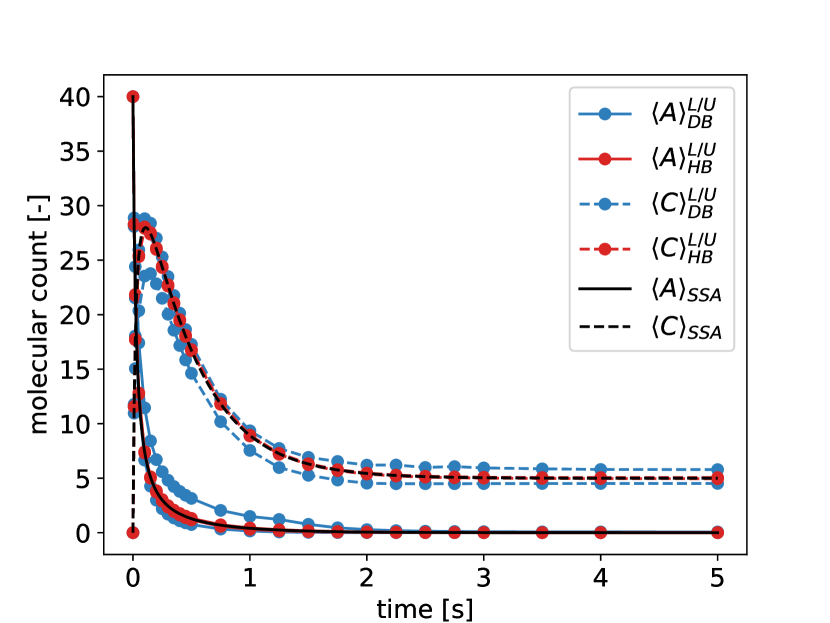
(a)

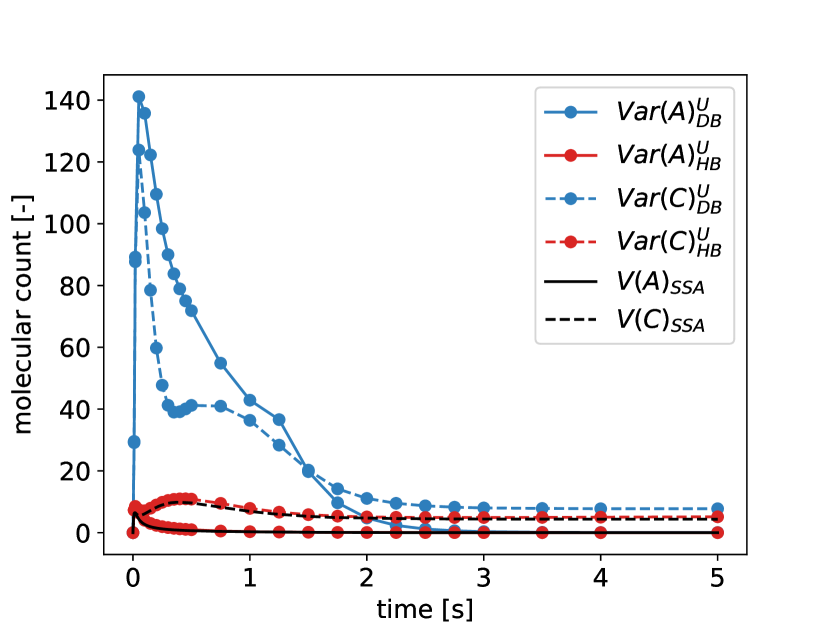
(b)

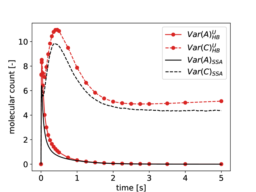
(c)

Figure 1: Bounds on (a) means and (b,c) variances of molecular counts of species A and C in reaction network (16); initial state: $x_{A,0}=40$, $x_{B,0}=41$, and $x_{C,0}=x_{D,0}=0$; kinetic parameters: $\bm{c}=(1,2.1,0.3)\,${\mathrm{s}}^{-1}$$; hierarchy parameters: $m=4$, $n_{\mathsf{F}}=3$, $n_{\mathsf{T}}=10$.

V.2.2 Cyclic Reaction Network

Second, we investigate the cyclic reaction network illustrated in Figure 2.

Figure 2: Cyclic reaction network from Dowdy and Barton (2018b)

This reaction network exhibits similar characteristics as the simple network studied in the previous section, i.e., a bounded state space and two independent species. In contrast to the simple network, however, the situation is a bit more complex since the reaction is fully reversible. Therefore, the reachable set of the cyclic reaction network is at least as large as that of the simple network given an identical initial state.

Figure 2 shows a comparison between the bounds obtained from (SDP) and Dowdy and Barton’s method. Although the bounds are slightly looser than before, the results demonstrate again the potential of the proposed methodology.

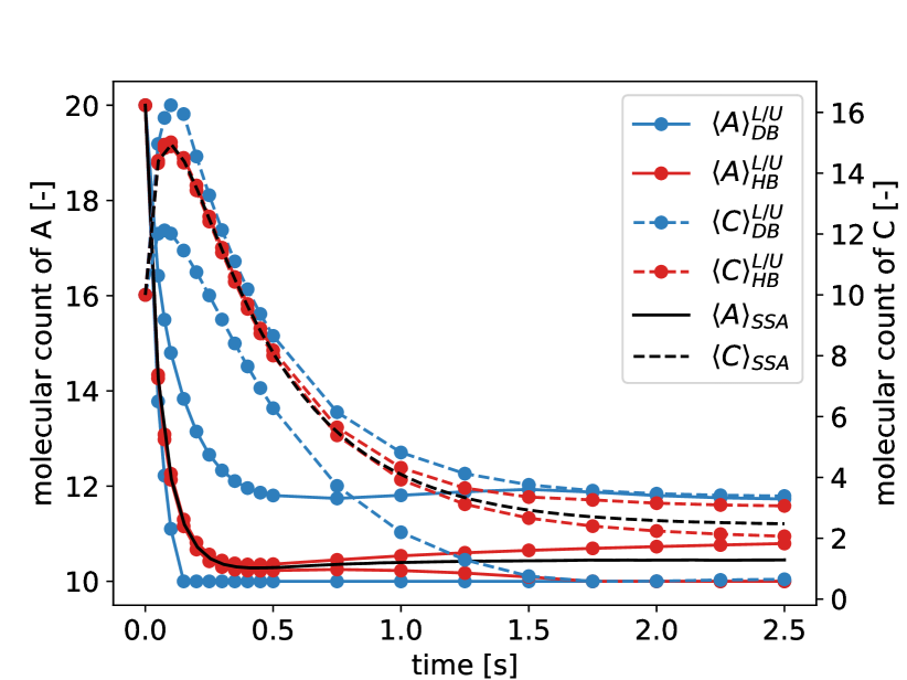
(a)

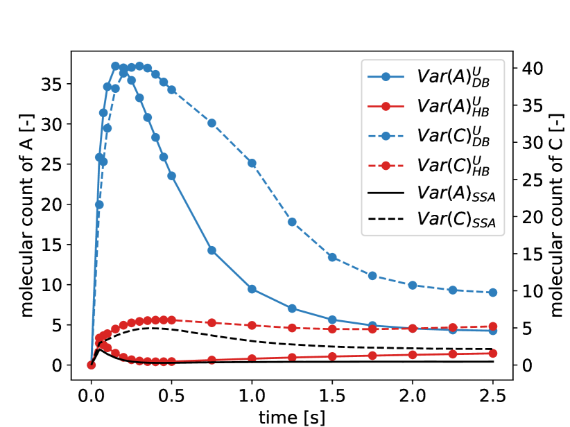
(b)

Figure 3: Bounds on means (a) and variances (b) of the molecular counts of species A and C in the cyclic reaction network shown in Figure 2; initial state: $x_{A,0}=20$, $x_{B,0}=10$, and $x_{C,0}=10$, $x_{D,0}=0$; kinetic parameters: $\bm{c}=(1,2.1,0.3)\,${\mathrm{s}}^{-1}$$; hierarchy parameters: $m=2$, $n_{\mathsf{F}}=3$, $n_{\mathsf{T}}=10$.

V.2.3 Large Reaction Network

Last, we investigate the reaction network illustrated in Figure 4. In contrast to the previous networks, this large reaction network poses a challenge for sampling based analysis techniques. The underlying reason for that is two-fold. On the one hand, the network is characterized by a large, 7-dimensional state space. On the other hand, the system is extremely stiff. These properties frustrate sampling based techniques as they exacerbate the need for large sample sizes and render each sample evaluation expensive.

Figure 5 shows bounds on the mean molecular counts of species $A$ and $H$. In line with the results of the previous sections, the bounds obtained by the proposed method are again considerably tighter. In this example, however, this result carries more weight as increasing the truncation order leads to a prohibitive increase in problem size for the method of Dowdy and Barton (2018b). Accordingly, the proposed method offers bounds at a quality that was previously not attainable for problems of such complexity.

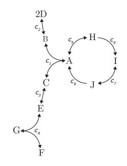
Figure 4: Large reaction network from Dowdy and Barton (2018b)

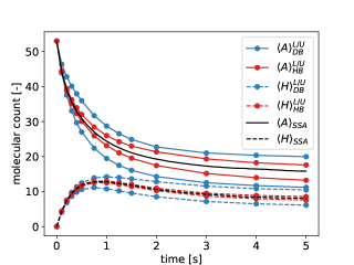
Figure 5: Bounds on the mean molecular counts of species A and H in the large reaction network shown in Figure 4; initial state: $x_{\ce{A},0}=x_{\ce{F},0}=53$, $x_{\ce{B},0}=x_{\ce{C},0}=x_{\ce{D},0}=x_{\ce{E},0}=x_{\ce{G},0}=x_{\ce{H},0}=x_{\ce{I},0}=x_{\ce{J},0}=0$; kinetic parameters: $\bm{c}=(1,1,1,10^{4},1,1,10^{5},1)\,${\mathrm{s}}^{-1}$$; hierarchy parameters: $m=2$, $n_{\mathsf{F}}=5$, $n_{\mathsf{T}}=5$.

V.3 Open Systems

We now depart from systems that have a bounded state space and turn to open systems. Such systems are of particular interest as their moments can rarely be found analytically and the corresponding CME gives rise to a countably infinite system of coupled ODEs precluding a direct numerical integration. To showcase the ability to compute tight moment bounds for systems of this type, we study two birth-death processes with different “degrees of nonlinearity”.

The first system we investigate is the following simple nonlinear birth-death process:

$$\emptyset\stackrel{{\scriptstyle c_{1}}}{{\rightarrow}}\ce{A},\qquad 2\ce{A}\stackrel{{\scriptstyle c_{2}}}{{\rightarrow}}\emptyset$$ (17)

Figure 6 draws a comparison between the bounds for the mean and variance of the molecular count of species A. The proposed method again yields substantially tighter bounds than its predecessor. In fact, the bounds on the mean are even tight enough to essentially recover the true solution.

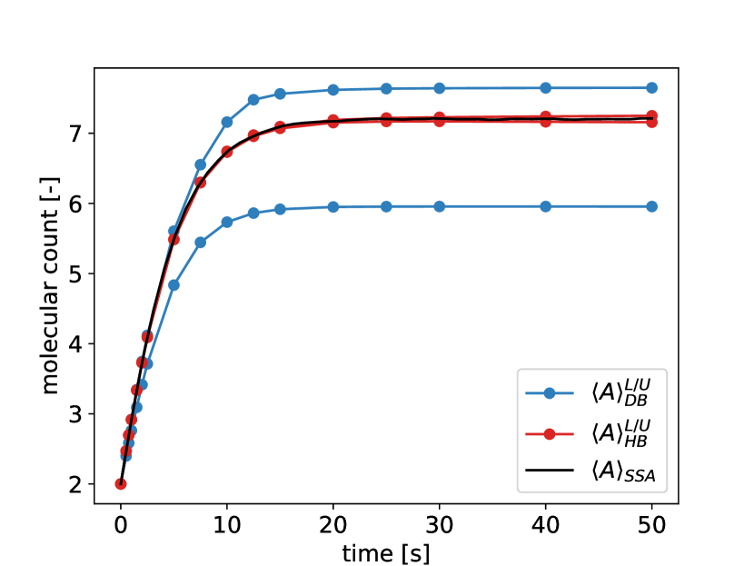
(a)

(b)

Figure 6: Bounds on means (a) and variances (b) of the molecular count of species A undergoing the birth-death process (17); initial state: $x_{A,0}=2$; kinetic parameters: $\bm{c}=(1,0.01)\,${\mathrm{s}}^{-1}$$; hierarchy parameters: $m=8$, $n_{\mathsf{F}}=3$, $n_{\mathsf{T}}=20$.

Next, we will consider Schlögl’s system Schlögl (1972):

$$2\ce{X}\stackrel{{\scriptstyle[}}{{c}}_{1}]{c_{2}}{\leftrightharpoons}3\ce{X},\qquad\ce{X}\stackrel{{\scriptstyle[}}{{c}}_{3}]{c_{4}}{\leftrightharpoons}\emptyset.$$ (18)

As a canonical example for a chemical bifurcation, Schlögel’s system was previously studied by different authors Dowdy and Barton (2018a); Kuntz et al. (2019) to illustrate bounding methods for the moments of stationary solutions of the CME. We provide the first analysis for the dynamic case here.

Figure 7 illustrates the results for Schlögl’s system. Although the proposed methodology again strongly outperforms its predecessor, the obtained bounds are rather loose. We emphasize, however, that we could not reproduce bounds of similar quality by increasing the truncation order in Dowdy and Barton’s Dowdy and Barton (2018b) method. The bounds started stalling before eventually poor numerical conditioning prohibited solution of the SDPs altogether.

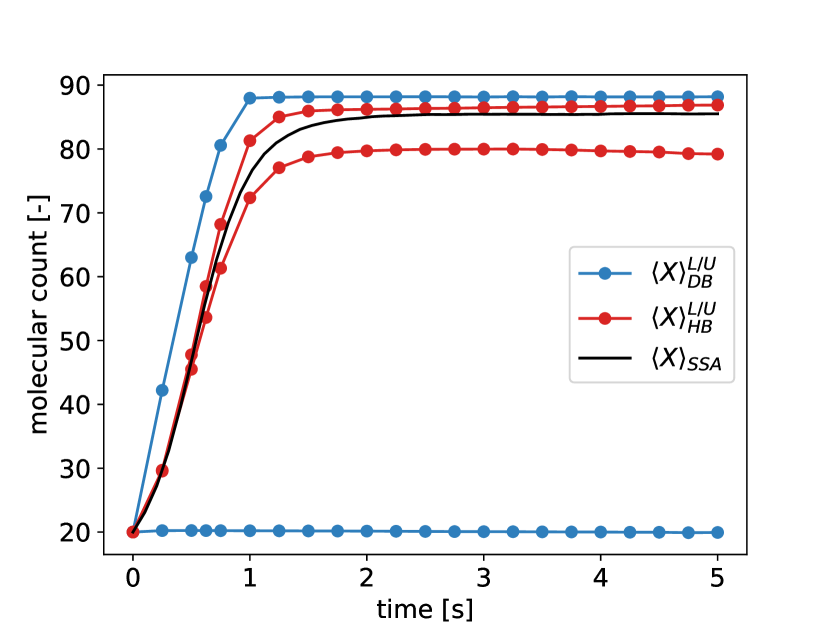
(a)

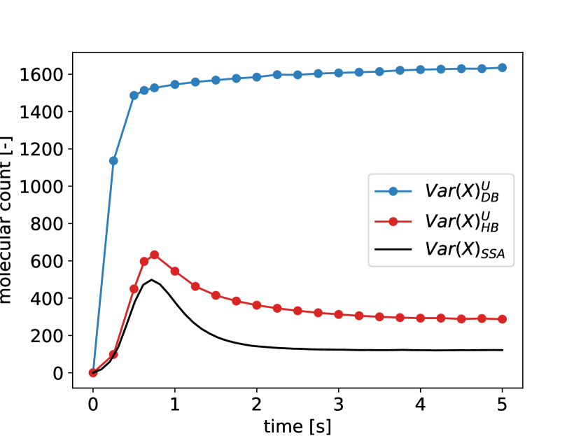
(b)

Figure 7: Bounds on means (a) and variances (b) of molecular counts of species X in Schlögl’s system (18); initial state: $x_{X,0}=20$; kinetic parameters: $\bm{c}=(0.15,$1.5\text{\times}{10}^{-3}\text{\,}\mathrm{,}$20,2)\,${\mathrm{s}}^{-1}$$; hierarchy parameters: $m=6$, $n_{\mathsf{F}}=3$, $n_{\mathsf{T}}=20$.

V.4 Biochemical Reaction Networks

To finally demonstrate that the proposed methodology may be useful in practice, we examine three reaction networks drawn from biochemical application. In these applications, molecular counts are often present in the order of 10s to 100s necessitating the consideration of stochasticity.

V.4.1 Michaelis-Menten Kinetics

Michaelis-Menten kinetics underpin a vast range of metabolic processes. Understanding the behavior and noise present in the associated reaction networks is of particular value for the investigation of the metabolic degradation of trace substances in biological organisms. We examine the basic Michaelis-Menten reaction network:

$$\ce{S}+\ce{E}\stackrel{{\scriptstyle[}}{{c}}_{1}]{c_{2}}{\leftrightharpoons}\ce{S}:\ce{E}\stackrel{{\scriptstyle c_{3}}}{{\rightarrow}}\ce{P}+\ce{E}$$

$$\ce{S}:\ce{E}\stackrel{{\scriptstyle c_{3}}}{{\rightarrow}}\ce{P}+\ce{E}$$ (19)

$$\ce{P}\stackrel{{\scriptstyle c_{4}}}{{\rightarrow}}\ce{S}$$

The reaction network features a two-dimensional state space. Accordingly, we bound the means and variances of the molecular counts of the product P and substrate S. The results are illustrated in Figure 8. For the sake of completeness, Figure 8 also features a comparison with the bounds obtained by Dowdy and Barton’s Dowdy and Barton (2018b) method. The proposed method reproduces essentially the exact solution for the means while providing reasonably tight bounds for the variances. Further, it again outperforms its predecessor, especially for bounds on the variances.

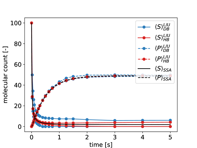
(a)

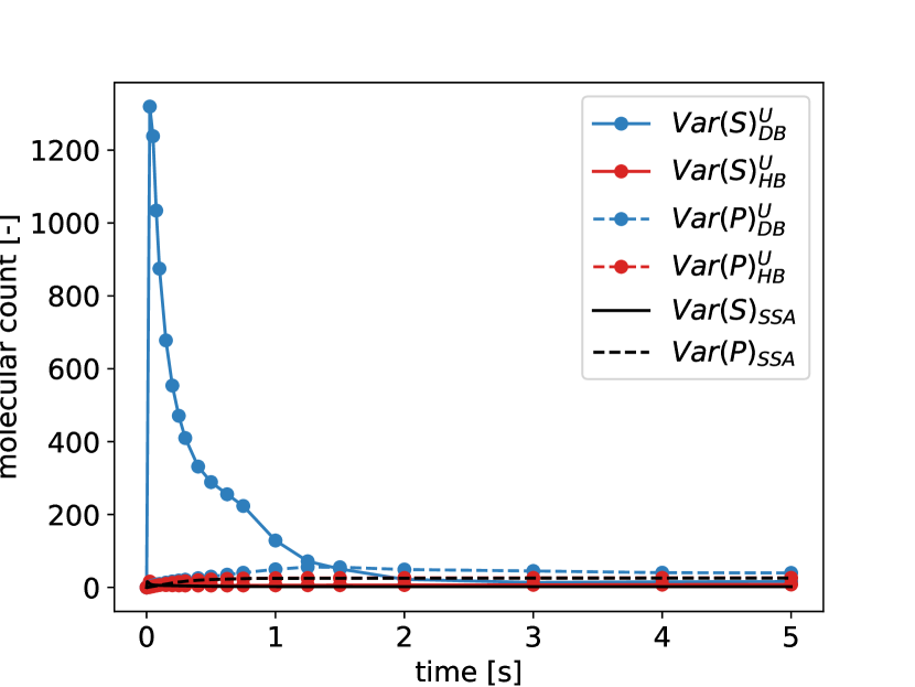
(b)

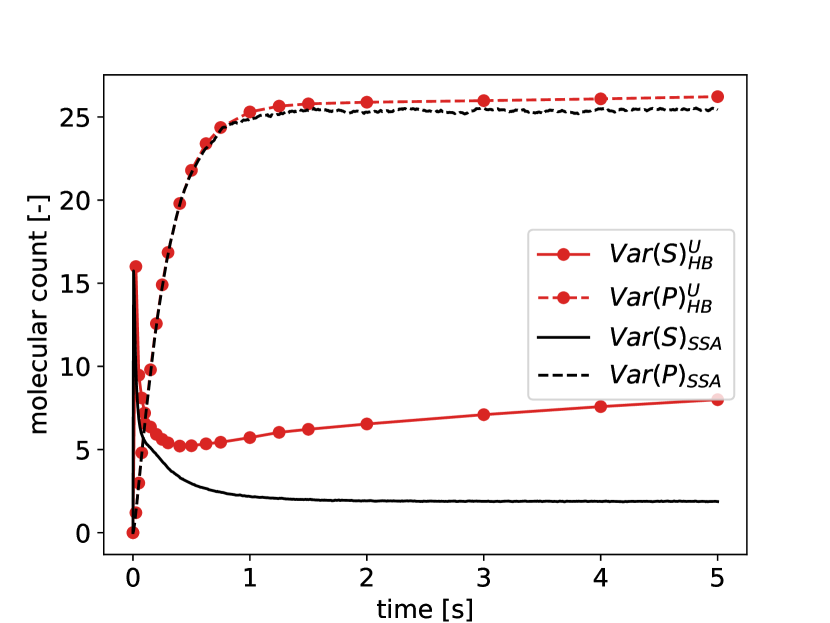
(c)

Figure 8: Bounds on means (a) and variances (b,c) of the molecular counts of species S and P in the metabolic reaction network (19); initial state: $x_{\ce{S},0}=x_{\ce{E},0}=100$, $x_{\ce{P},0}=x_{\ce{S}:\ce{E},0}=0$; kinetic parameters: $\bm{c}=(1,1,1,1)\,${\mathrm{s}}^{-1}$$; hierarchy parameters: $m=4$, $n_{\mathsf{F}}=3$, $n_{\mathsf{T}}=20$.

V.4.2 Negative Feedback Biocircuit

Many efforts of modern synthetic biology culminate in the design of biocircuits subject to stringent constraints on robustness and performance. Upon successful design, the implications of such tailored biocircuits are often far reaching, even addressing global challenges such as water pollution Sinha, Reyes, and Gallivan (2010) and energy Peralta-Yahya et al. (2012). Accordingly, in recent years the use of systems theoretic techniques has received considerable attention to conceptualize, better understand and speed up the design process of biocircuits Del Vecchio, Dy, and Qian (2016). In this context, Sakurai and Hori (2018) demonstrated the utility of stationary moment bounds for the design of biocircuits subject to robustness constraints. Here, we demonstrate that the proposed methodology could enable an extension of their analysis to the dynamic case.

We examine the negative feedback biocircuit illustrated in Figure 9 studied by Sakurai and Hori (2018). The corresponding reaction network is given by

$$\begin{array}[]{l}\ce{DNA}\stackrel{{\scriptstyle c_{1}}}{{\rightarrow}}\ce{DNA}+\ce{mRNA}\\ \ce{mRNA}\stackrel{{\scriptstyle c_{2}}}{{\rightarrow}}\emptyset\\ \ce{mRNA}\stackrel{{\scriptstyle c_{3}}}{{\rightarrow}}\ce{mRNA}+\ce{P}\\ \ce{P}\stackrel{{\scriptstyle c_{4}}}{{\rightarrow}}\emptyset\\ \ce{P}+\ce{DNA}\stackrel{{\scriptstyle[}}{{c}}_{6}]{c_{5}}{\rightleftharpoons}\ce{P}:\ce{DNA}\end{array}.$$ (25)

Figure 10 illustrates the obtained bounds on means and variance of the molecular counts of the species mRNA and P. The bounds are of high quality and may provide useful information for robustness analysis as the noise level measured by the variance changes significantly over the time horizon until the steady-state value is reached.

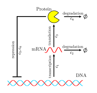
Figure 9: Negative feedback biocircuit from Sakurai and Hori (2018)

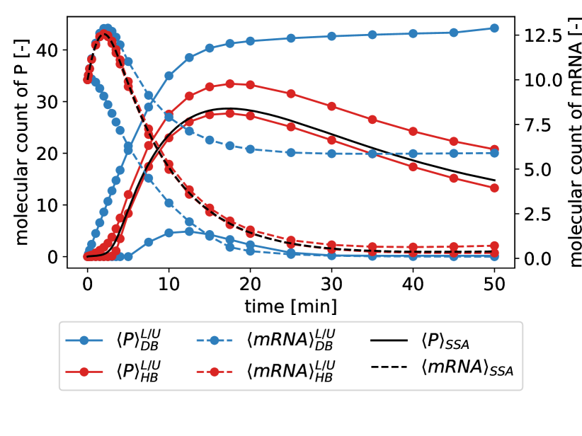
(a)

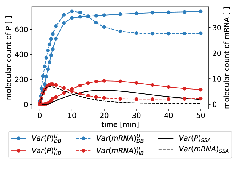
(b)

Figure 10: Bounds on means (a) and variances (b) of the molecular counts of $\ce{mRNA}$ and $P$ in the negative feedback biocircuit illustrated in Figure 9; initial state: $x_{\ce{mRNA},0}=10$, $x_{\ce{P},0}=x_{\ce{P}:\ce{DNA},0}=0$, $x_{\ce{DNA},0}=20$; kinetic parameters: $\bm{c}=(0.2,\ln(2)/5,0.5,\ln(2)/20,5,1)\,${\mathrm{min}}^{-1}$$; hierarchy parameters: $m=4$, $n_{\mathsf{F}}=3$, $n_{\mathsf{T}}=20$.

V.4.3 Viral Infection

As our last example we consider the following reaction network from Srivastava et al. (2002) used to model for the intracellular kinetics of a virus:

$$\begin{array}[]{lll}\ce{G}\stackrel{{\scriptstyle c_{1}}}{{\rightarrow}}\ce{T},&\ce{T}\stackrel{{\scriptstyle c_{2}}}{{\rightarrow}}\emptyset,&\ce{T}\stackrel{{\scriptstyle c_{3}}}{{\rightarrow}}\ce{T}+\ce{G}\\ \ce{G}+\ce{S}\stackrel{{\scriptstyle c_{4}}}{{\rightarrow}}\emptyset,&\ce{T}\stackrel{{\scriptstyle c_{5}}}{{\rightarrow}}\ce{T}+\ce{S},&\ce{S}\stackrel{{\scriptstyle c_{6}}}{{\rightarrow}}\emptyset\end{array}.$$ (28)

In this network, S represents the viral structural protein while T and G represent the viral nucleic acids categorized as template and genomic, respectively.

Studying a system undergoing the reactions as described by the above network with sampling based approaches is computationally expensive. This is due to two distinct reasons. On the one hand, the state space is infinite. On the other hand, the molecular counts of S, T and G vary over several orders of magnitude so that they evolve at different time scales and noise levels. This characteristic is found in many biochemical reaction networks and has motivated the development of hybrid simulation techniques; see for example Haseltine and Rawlings (2002). Such hybrid approaches combine the use of deterministic models for the dynamics of species present at large counts with stochastic models for rare events and species present at low counts. Although such methods accelerate simulation substantially, they generally introduce a range of assumptions accompanied by an unknown error. The methodology presented in this article provides a framework to quantify this error. Figure 11 shows the bounds obtained for the mean molecular counts of all three species. Although the bounds are not tight, we argue that they may be informative enough to assess whether approximate solutions are reasonable. This in stark contrast to Dowdy and Barton’s method Dowdy and Barton (2018b) which in this case provides extremely loose bounds that could not be substantially improved due to numerical difficulties and prohibitive computational cost at high truncation orders.

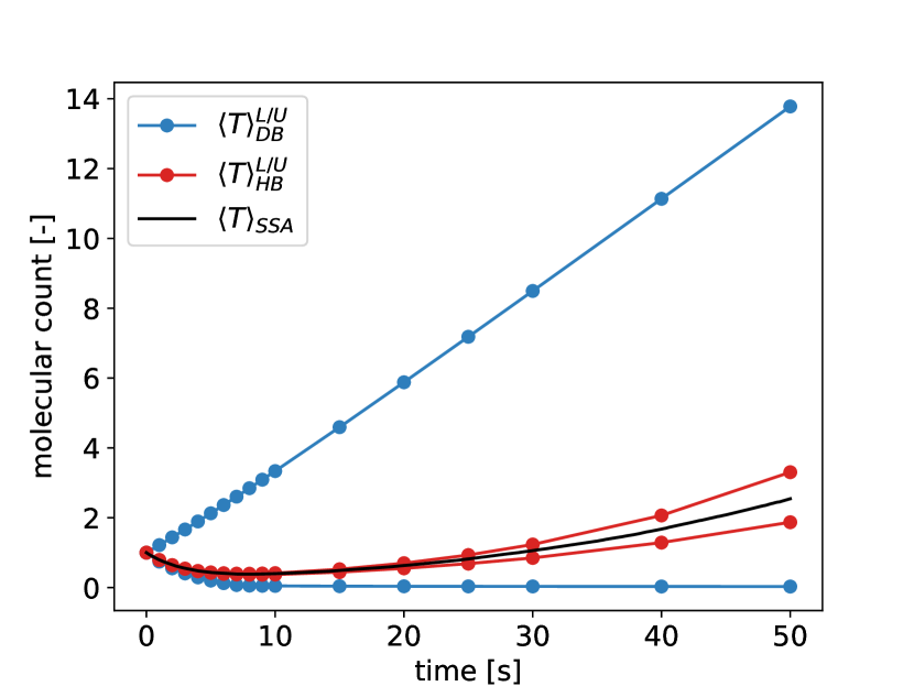
(a)

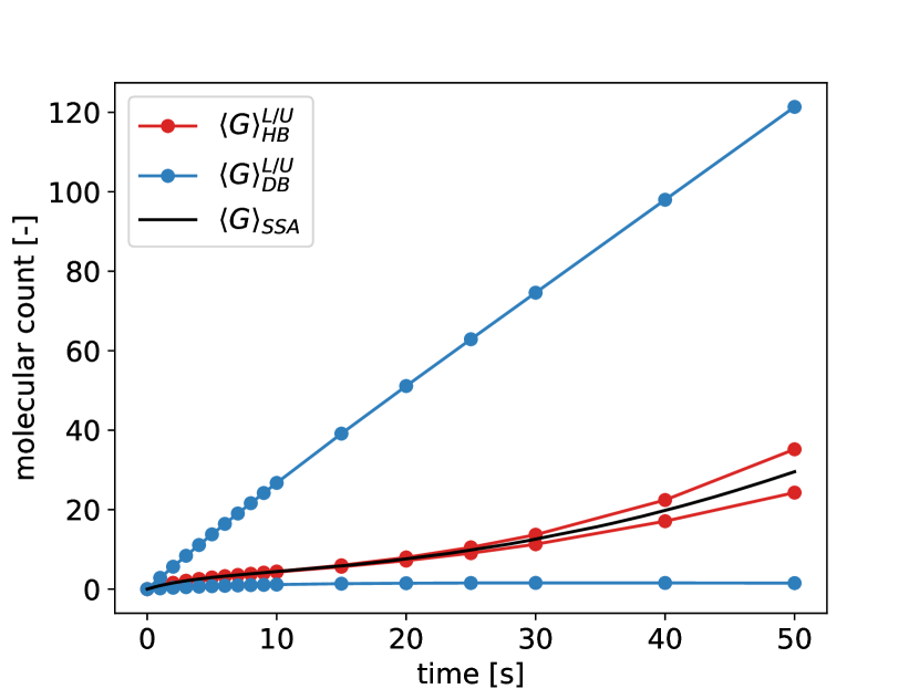
(b)

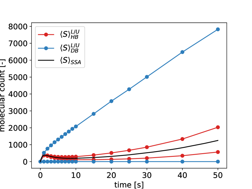
(c)

Figure 11: Bounds on mean molecular counts of Template (a), Genome (b) and Struct (c) species in the viral infection network (28); initial state: $x_{\ce{T},0}=1$, $x_{\ce{G},0}=x_{\ce{S},0}=0$; kinetic parameters: $\bm{c}=(0.025,0.25,1,$7.5\text{\times}{10}^{-6}\text{\,}\mathrm{,}$$1\text{\times}{10}^{3}\text{\,}\mathrm{,}$1.99)\,${\mathrm{d}}^{-1}$$; hierarchy parameters: $m=4$, $n_{\mathsf{F}}=3$, $n_{\mathsf{T}}=20$.

VI Bound Tightening Mechanisms

In this section, we briefly assess the effect of the different bound tightening mechanisms provided by the proposed bounding hierarchy. We conduct this empirical analysis on the basis of the birth-death process (17). Furthermore, we restrict our considerations here to studying the effect of increasing the truncation order $m$, the hierarchy level $n_{I}$ and the number of time points $n_{\mathsf{T}}$ used to discretize the horizon; throughout, we only use the constant test function ($n_{\mathsf{F}}=1$).

Figure 12 shows the effect of isolated changes in the different hierarchy parameters on the bounds obtained for the mean molecular count and its variance. The results indicate that all bound tightening mechanisms, when used in isolation, appear to suffer from diminishing returns, eventually causing the bounds to stall. Moreover, solely increasing the truncation order $m$ appears insufficient to provide informative bounds over a long time horizon in this example; increasing either the number of time points or the hierarchy level $n_{I}$ are significantly more effective in comparison.

Figure 13 shows the effect of joint changes in the considered hierarchy parameters on the tightness of bounds on the mean molecular count. The figure indicates that jointly changing the hierarchy parameters effectively mitigates stalling of the bounds in this example such that significantly tighter bounds are obtained overall. While the general trends illustrated by Figures 12 and 13 align well with our experiences for a range of other examples, we wish to emphasize that it is in general hard to predict which combination of hierarchy parameters provides the best trade-off between computational cost and bound quality; when the choice of test functions is added to the equation, the situation becomes even more complicated. Moreover, as Figure 14 illustrates, the feasible region of the bounding SDPs shrinks anisotropically and, more importantly, with different intensity along different directions for different bound tightening mechanisms. As a consequence, the optimal choice of the hierarchy parameters is in general not only dependent on the system under investigation but also on the statistical quantity to be bounded.

In summary, the results presented in this section underline the value of the additional bound tightening mechanisms offered by the proposed hierarchy; however, they also emphasize the need for better guidelines to enable an effective use of the tightening mechanisms in practice.

(a) $n_{I}=2$, $n_{\mathsf{T}}=2$

(b) $n_{I}=2$, $n_{\mathsf{T}}=2$

(c) $m=2$, $n_{\mathsf{T}}=2$

(d) $m=2$, $n_{\mathsf{T}}=2$

(e) $m=2$, $n_{I}=2$

(f) $m=2$, $n_{I}=2$

Figure 12: Bounds on the trajectories of the mean molecular count and variance of the birth-death process (17) for increasing $m$ (a,b), $n_{I}$ (c,d), and $n_{\mathsf{T}}$ (e,f) compared against the empiric sample mean and variance generated with Gillespie’s SSA. In each figure only one parameter is varied while the others are held constant at the level indicated in the subcaptions.

(a) $n_{\mathsf{T}}=2$

(b) $n=2$

(c) $m=2$

Figure 13: Maximum gap between upper and lower bounds on mean molecular counts among the time points probed along the time horizon for joint changes in $m$ and $n_{I}$ (a), $m$ and $n_{\mathsf{T}}$ (b), and $n_{I}$ and $n_{\mathsf{T}}$ (c).

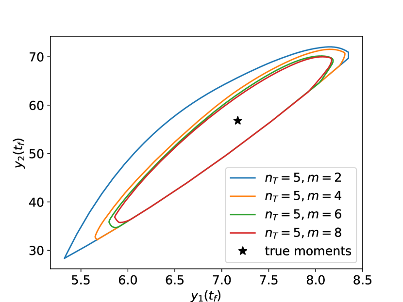
(a)

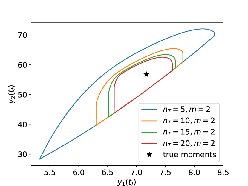
(b)

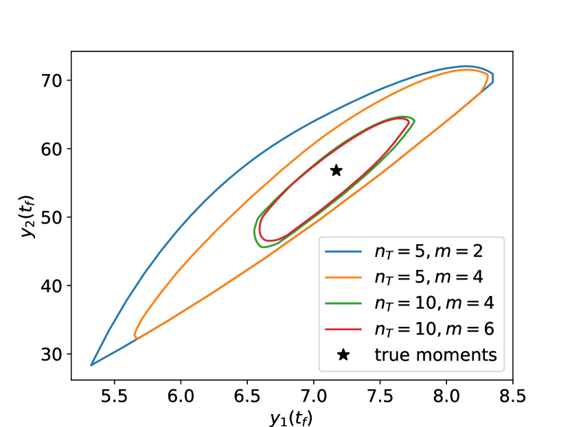
(c)

Figure 14: Projection of the feasible set of (SDP) corresponding to the birth-death process (17) for (a) increasing truncation order, (b) increasing number of time points $n_{\mathsf{T}}$, and (c) jointly increasing truncation order and number of time points. All projections are obtained for $n_{I}=2$ and $t_{f}=20$.

VII Conclusion

VII.1 Summary

We have extended the results of Dowdy and Barton (2018b) by constructing a new hierarchy of convex necessary moment conditions for the moment trajectories of stochastic chemical systems described by the CME. Building on a discretization of the time domain of the problem, the conditions reflect temporal causality and regularity properties of the true moment trajectories. It is proved that the conditions give rise to a hierarchy of highly structured SDPs whose optimal values form a sequence of monotonically improving bounds on the true moment trajectories. Furthermore, the conditions provide new mechanisms to tighten the obtained bounds when compared to the original conditions proposed by Dowdy and Barton (2018b). These tightening mechanisms are often a substantially more scalable alternative to the primary tightening mechanism of increasing the truncation order in Dowdy and Barton’s approach Dowdy and Barton (2018b); most notably, refining the time discretization results in linearly increasing problem sizes, independent of the state space dimension of the system. As an additional advantage, this bound tightening mechanism provides a way to sidestep the poor numerical conditioning of moment-based SDPs featuring high-order moments. Finally, it is demonstrated with several examples that the proposed hierarchy provides bounds that may indeed be useful in practice.

VII.2 Open Questions

We close by stating some open questions motivated by our results.

1. In the presented case studies, we naively chose the time points at which the proposed necessary moment conditions were imposed as equidistant. Several results from numerical integration, perhaps most notably Gauß quadrature, suggest that this is likely not the optimal choice. It would be interesting to examine if and how results from numerical integration can inform improvements of this choice.

2. The choice of the hierarchy parameters in the proposed bounding scheme is crucial to achieve a good trade-off between bound quality and computational cost. As indicated by the discussion in Section VI, however, the interplay between the bound tightening mechanisms associated with the different hierarchy parameters and their effect on the bound quality remains poorly understood. Accordingly, we believe that assessing the trade-offs offered by the different bound tightening mechanisms in greater detail and developing more rigorous guidelines on how to utilize them effectively constitutes an important step towards improving the practicality of the proposed method.

3. The ideas discussed in Section IV constitute promising research avenues towards improving practicality of the proposed method. Specifically, there are several open questions pertaining to the concrete implementation of Algorithm 1 and the way Problem (pwpOCP) can be used to inform an effective use of the different bound tightening mechanisms. Furthermore, the decomposable, weakly coupled structure of the bounding SDPs motivates other forms of exploitation than Algorithm 1; in particular the use of distributed optimization techniques such as ADMM Boyd et al. (2011) or Schwarz-like approaches Shin, Zavala, and Anitescu (2020); Na et al. (2020) appears promising.

Supplementary Information

The Supplementary Information to this article can be found at the end of this document.

References

References

- Arkin, Ross, and McAdams (1998) A. Arkin, J. Ross, and H. H. McAdams, “Stochastic kinetic analysis of developmental pathway bifurcation in phage -infected Escherichia coli cells,” Genetics 149, 1633–1648 (1998).
- Elowitz et al. (2002) M. B. Elowitz, A. J. Levine, E. D. Siggia, and P. S. Swain, “Stochastic gene expression in a single cell,” Science 297, 1183–1186 (2002).
- Liu and Jia (2004) Q. Liu and Y. Jia, “Fluctuations-induced switch in the gene transcriptional regulatory system,” Physical Review E 70, 41907 (2004).
- Artyomov et al. (2007) M. N. Artyomov, J. Das, M. Kardar, and A. K. Chakraborty, “Purely stochastic binary decisions in cell signaling models without underlying deterministic bistabilities,” Proceedings of the National Academy of Sciences 104, 18958–18963 (2007).
- Gillespie (1976) D. T. Gillespie, “A General Method for Numerically Simulating the Stochastic Time Evolution of Coupled Chemical Reactions,” Journal of Computational Physics 22, 403–434 (1976).
- Gillespie (1977) D. T. Gillespie, “Exact stochastic simulation of coupled chemical reactions,” The Journal of Physical Chemistry 81, 2340–2361 (1977).
- Gillespie, Hellander, and Petzold (2013) D. T. Gillespie, A. Hellander, and L. R. Petzold, “Perspective: Stochastic algorithms for chemical kinetics,” The Journal of Chemical Physics 138, 05B201_1 (2013).
- Munsky and Khammash (2006) B. Munsky and M. Khammash, “The finite state projection algorithm for the solution of the chemical master equation,” The Journal of Chemical Physics 124, 44104 (2006).
- Ale, Kirk, and Stumpf (2013) A. Ale, P. Kirk, and M. P. H. Stumpf, “A general moment expansion method for stochastic kinetic models,” The Journal of Chemical Physics 138, 174101 (2013).
- Keeling (2000) M. J. Keeling, “Multiplicative moments and measures of persistence in ecology,” Journal of Theoretical Biology 205, 269–281 (2000).
- Nåsell (2003) I. Nåsell, “An extension of the moment closure method,” Theoretical Population Biology 64, 233–239 (2003).
- Smadbeck and Kaznessis (2013) P. Smadbeck and Y. N. Kaznessis, “A closure scheme for chemical master equations,” Proceedings of the National Academy of Sciences 110, 14261–14265 (2013).
- Schnoerr, Sanguinetti, and Grima (2015) D. Schnoerr, G. Sanguinetti, and R. Grima, “Comparison of different moment-closure approximations for stochastic chemical kinetics,” The Journal of Chemical Physics 143, 11B610_1 (2015).
- Schnoerr, Sanguinetti, and Grima (2014) D. Schnoerr, G. Sanguinetti, and R. Grima, “Validity conditions for moment closure approximations in stochastic chemical kinetics,” The Journal of Chemical Physics 141, 08B616_1 (2014).
- Grima (2012) R. Grima, “A study of the accuracy of moment-closure approximations for stochastic chemical kinetics,” The Journal of Chemical Physics 136, 04B616 (2012).
- Dowdy and Barton (2018a) G. R. Dowdy and P. I. Barton, “Bounds on stochastic chemical kinetic systems at steady state,” The Journal of chemical physics 148, 84106 (2018a).
- Ghusinga et al. (2017) K. R. Ghusinga, C. A. Vargas-Garcia, A. Lamperski, and A. Singh, “Exact lower and upper bounds on stationary moments in stochastic biochemical systems,” Physical Biology 14, 04LT01 (2017).
- Kuntz et al. (2019) J. Kuntz, P. Thomas, G.-B. Stan, and M. Barahona, “Bounding the stationary distributions of the chemical master equation via mathematical programming,” The Journal of Chemical Physics 151, 34109 (2019).
- Sakurai and Hori (2017) Y. Sakurai and Y. Hori, “A convex approach to steady state moment analysis for stochastic chemical reactions,” in 2017 IEEE 56th Annual Conference on Decision and Control (CDC) (IEEE, 2017) pp. 1206–1211.
- Dowdy and Barton (2018b) G. R. Dowdy and P. I. Barton, “Dynamic bounds on stochastic chemical kinetic systems using semidefinite programming,” The Journal of Chemical Physics 149, 74103 (2018b).
- Sakurai and Hori (2019) Y. Sakurai and Y. Hori, “Bounding transient moments of stochastic chemical reactions,” IEEE Control Systems Letters 3, 290–295 (2019).
- Del Vecchio, Dy, and Qian (2016) D. Del Vecchio, A. J. Dy, and Y. Qian, “Control theory meets synthetic biology,” Journal of The Royal Society Interface 13, 20160380 (2016).
- Backenköhler, Bortolussi, and Wolf (2019) M. Backenköhler, L. Bortolussi, and V. Wolf, “Bounding First Passage Times in Chemical Reaction Networks,” in International Conference on Computational Methods in Systems Biology (Springer, 2019) pp. 379–382.
- Sakurai and Hori (2018) Y. Sakurai and Y. Hori, “Optimization-based synthesis of stochastic biocircuits with statistical specifications,” Journal of the Royal Society Interface 15, 20170709 (2018).
- Resnick (1992) S. I. Resnick, Adventures in stochastic processes (Springer Science & Business Media, 1992).
- Gillespie (1992) D. T. Gillespie, “A rigorous derivation of the chemical master equation,” Physica A: Statistical Mechanics and its Applications 188, 404–425 (1992).
- Gillespie (2009) C. S. Gillespie, “Moment-closure approximations for mass-action models,” IET Systems Biology 3, 52–58 (2009).
- Lasserre (2001) J. B. Lasserre, “Global Optimization with Polynomials and the Problem of Moments,” SIAM Journal on Optimization 11, 796–817 (2001).
- Lasserre (2010) J. B. Lasserre, Moments, Positive Polynomials and Their Applications, Vol. 1 (World Scientific, 2010).
- Note (1) If or grow too large, the Taylor polynomial or remainder may depend on moments of higher order than but the dependence will still be linear.
- Andersen and Andersen (2000) E. Andersen and K. Andersen, “The MOSEK interior point optimizer for linear programming: an implementation of the homogeneous algorithm,” in High Performance Optimization (Springer, 2000) pp. 197–232.
- Sturm (1999) J. F. Sturm, “Using SeDuMi 1.02, a MATLAB toolbox for optimization over symmetric cones,” Optimization Methods and Software 11, 625–653 (1999).
- Toh, Todd, and Tütüncü (1999) K.-C. Toh, M. J. Todd, and R. H. Tütüncü, “SDPT3—a MATLAB software package for semidefinite programming, version 1.3,” Optimization Methods and Software 11, 545–581 (1999).
- Ahmadi, Dash, and Hall (2017) A. A. Ahmadi, S. Dash, and G. Hall, “Optimization over structured subsets of positive semidefinite matrices via column generation,” Discrete Optimization 24, 129–151 (2017).
- Ahmadi and Hall (2019) A. A. Ahmadi and G. Hall, “On the construction of converging hierarchies for polynomial optimization based on certificates of global positivity,” Mathematics of Operations Research 44, 1192–1207 (2019).
- Braun et al. (2015) G. Braun, S. Fiorini, S. Pokutta, and D. Steurer, “Approximation limits of linear programs (beyond hierarchies),” Mathematics of Operations Research 40, 756–772 (2015).
- Ahmadi and Majumdar (2019) A. A. Ahmadi and A. Majumdar, “DSOS and SDSOS Optimization: More Tractable Alternatives to Sum of Squares and Semidefinite Optimization,” SIAM Journal on Applied Algebra and Geometry 3, 193–230 (2019).
- Bertsimas and Cory-Wright (2020) D. Bertsimas and R. Cory-Wright, “On polyhedral and second-order cone decompositions of semidefinite optimization problems,” Operations Research Letters 48, 78–85 (2020).
- Rudin (1976) W. Rudin, Principles of mathematical analysis, Vol. 3 (McGraw-Hill, New York, 1976).
- Ahmadi and Khadir (2018) A. A. Ahmadi and B. E. Khadir, “Time-varying semidefinite programs,” arXiv preprint arXiv:1808.03994 , 1–33 (2018).
- Cuthrell and Biegler (1987) J. E. Cuthrell and L. T. Biegler, “On the Optimization of Differential-Algebraic Process Systems,” AIChE Journal 33, 1257–1270 (1987).
- Dunning, Huchette, and Lubin (2017) I. Dunning, J. Huchette, and M. Lubin, “JuMP: A Modeling Language for Mathematical Optimization,” SIAM Review 59, 295–320 (2017).
- Schlögl (1972) F. Schlögl, “Chemical reaction models for non-equilibrium phase transitions,” Zeitschrift für Physik 253, 147–161 (1972).
- Sinha, Reyes, and Gallivan (2010) J. Sinha, S. J. Reyes, and J. P. Gallivan, “Reprogramming bacteria to seek and destroy an herbicide,” Nature Chemical Biology 6, 464 (2010).
- Peralta-Yahya et al. (2012) P. P. Peralta-Yahya, F. Zhang, S. B. Del Cardayre, and J. D. Keasling, “Microbial engineering for the production of advanced biofuels,” Nature 488, 320–328 (2012).
- Srivastava et al. (2002) R. Srivastava, L. You, J. Summers, and J. Yin, “Stochastic vs. deterministic modeling of intracellular viral kinetics,” Journal of Theoretical Biology 218, 309–321 (2002).
- Haseltine and Rawlings (2002) E. L. Haseltine and J. B. Rawlings, “Approximate simulation of coupled fast and slow reactions for stochastic chemical kinetics,” The Journal of Chemical Physics 117, 6959–6969 (2002).
- Boyd et al. (2011) S. Boyd, N. Parikh, E. Chu, B. Peleato, and J. Eckstein, “Distributed optimization and statistical learning via the alternating direction method of multipliers,” (2011).
- Shin, Zavala, and Anitescu (2020) S. Shin, V. M. Zavala, and M. Anitescu, “Decentralized schemes with overlap for solving graph-structured optimization problems,” IEEE Transactions on Control of Network Systems 7, 1225–1236 (2020).
- Na et al. (2020) S. Na, S. Shin, M. Anitescu, and V. M. Zavala, “Overlapping schwarz decomposition for nonlinear optimal control,” arXiv , 1–13 (2020).