Simulating near-field enhancement in transmission of airborne viruses with a quadrature-based model
Abstract
Airborne viruses, such as influenza, tuberculosis, and SARS-CoV-2, are transmitted through virus-laden particles expelled when an infectious person sneezes, coughs, talks, or breathes. These virus-laden particles are more highly concentrated in the expiratory jet of an infectious person than in a well-mixed room, but this near-field enhancement in virion exposure has not been well quantified. Transmission of airborne viruses depends on factors that are inherently variable and, in many cases, poorly constrained, and quantifying this uncertainty requires large ensembles of model simulations that span the variability in input parameters. However, models that are well-suited to simulate the near-field evolution of respiratory particles are also computationally expensive, which limits the exploration of parametric uncertainty. In order to perform many simulations that span the wide variability in factors governing transmission, we developed the Quadrature-based model of Respiratory Aerosol and Droplets (QuaRAD). QuaRAD is an efficient framework for simulating the evolution of virus-laden particles after they are expelled from an infectious person, their deposition to the nasal cavity of a susceptible person, and the subsequent risk of initial infection. We simulated 10,000 scenarios to quantify the risk of initial infection by a particular virus, SARS-CoV-2. The predicted risk of infection was highly variable among scenarios and, in each scenario, was strongly enhanced near the infectious individual. In more than 50% of scenarios, the physical distancing needed to avoid near-field enhancements in airborne transmission was beyond the recommended safe distance of two meters (six feet) if the infectious person is not wearing a mask, though this distance defining the near-field extent was also highly variable among scenarios. We find this variability in the near-field extent is explained predominantly by variability in expiration velocity. These findings suggest that, during outbreaks of airborne viruses, it is best to maintain at least three meters of distance to avoid local increases in virion exposure near an infectious person; protections against airborne transmission, such as N95 respirators, should be available for work conditions where distancing is not possible.
1 Introduction
Airborne transmission of pathogens was first recognized over fifty years ago (Riley et al.,, 1959) and has since been acknowledged as an important transmission route for a number of infectious diseases (Yu et al.,, 2004; Bloch et al.,, 1985; Zhao et al.,, 2019; Kim et al.,, 2016; Leclair et al.,, 1980). Even so, the risks posed by airborne spread remain poorly addressed by many safety standards (Bahl et al.,, 2020), a trend that continued with dire consequences during the early phases of the COVID-19 pandemic (Morawska and Milton,, 2020). It is now apparent that transmission of SARS-CoV-2, the virus causing COVID-19, occurs primarily through the airborne route (Samet et al.,, 2021; Prather et al.,, 2020). Though long-range airborne transmission is possible due to the small size and long transport distances of many infectious respiratory particles, the risk of infection is greatest near infectious individuals where the concentration of virions is highest (Meyerowitz et al.,, 2020). These near-field enhancements in transmission must be understood to design and implement effective mitigation strategies, such as selecting the distance needed between desks in a classroom or between workers in a factory. However, near-field increases in virion exposure are subject to variable and poorly constrained parameters, and this uncertainty in factors controlling transmission is not easily represented in models.
A key challenge in quantifying near-field effects is the inherent variability in factors governing transmission risk. For example, the rate at which different individuals expel virions varies by orders of magnitude (Chen et al.,, 2020; Leung et al.,, 2020), and epidemiological data suggests that the risk of infection at a given virion dose is also highly variable (Chen and Zheng,, 2020). These uncertainties in the physiological characteristics of both infectious and susceptible individuals leads to large uncertainty in predictions of transmission risk (Gale,, 2020; Watanabe et al.,, 2010). Large ensembles of model simulations are needed to quantify this uncertainty. However, while computational fluid dynamics models simulate air flows within a room in great detail and are, therefore, are able to resolve heterogeneity in virion concentrations (e.g. Beghein et al.,, 2005; Choi and Edwards,, 2012), these models are computationally expensive (e.g. Beghein et al.,, 2005; Choi and Edwards,, 2012), limiting the number of simulations that can be performed. Multi-zone models that simulate air flow within buildings typically track the average concentration in each room (e.g. Li et al.,, 2005; Emmerich et al.,, 1994); by assuming virions are well mixed within each room, these models neglect local increases in virion concentrations near an infectious person. To represent airborne transmission across a wide range of conditions, a model framework is needed that accurately represents processes governing near-field and far-field transmission but is efficient enough to perform large ensembles of simulations.
To address this need, we introduce the Quadrature-based model for Respiratory Aerosol and Droplets (QuaRAD), an efficient framework for simulating the full life cycle of virus-laden particles within indoor spaces — from their initial creation and expulsion from an infectious person to their eventual removal from the space or their deposition in the nasal passages of a new host. This model framework is an alternative to Monte Carlo models for simulating the dispersion and evolution of respiratory particles. In contrast to Monte Carlo models, which represent particle size distributions using thousands of randomly sampled particles, quadrature-based moment methods have been shown to accurately represent low-order distribution moments — as well as other integrated quantities — using only a small number of quadrature points (McGraw,, 1997; Fierce and McGraw,, 2017). In this study, the quadrature representation was used to quantify the rate at which particles deposit into the most likely initial infection site of SARS-CoV-2, the nasal epithelium. This paper describes the QuaRAD model (Section 2) and its application to simulation across a wide range of scenarios (Section 3). Though we focus here specifically on SARS-CoV-2, most aspects of this model are equally applicable and easily adaptable to studying the airborne transmission of any disease.
2 Model description
The respiratory particles that carry airborne viruses are created in the respiratory system through expiratory activities such as sneezing, coughing, talking, or breathing. A particle’s size at the time it is expelled dictates the distance it travels before settling to the ground. If a particle is transported to another individual and inhaled, its size influences if and where in the respiratory system it is most likely to deposit. For this reason, the QuaRAD model is designed to accurately and efficiently represent the size distribution of expelled particles and its evolution through evaporation, transport, and removal.
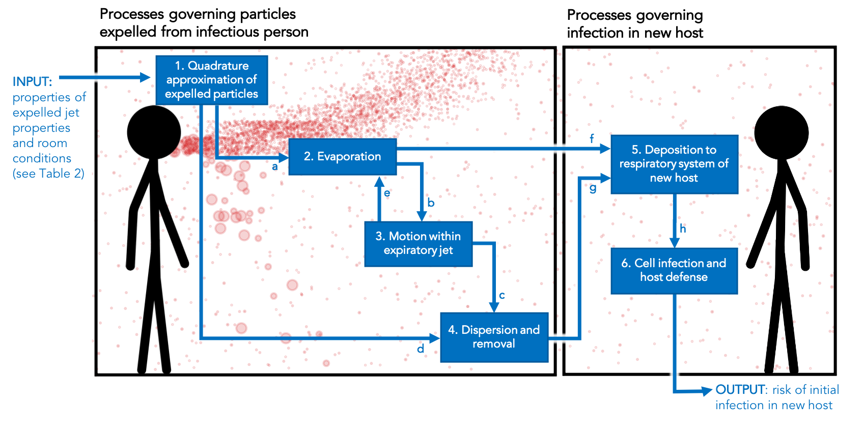
The processes simulated in QuaRAD are shown in Fig. 1. The model represents mechanisms governing the transport and evolution of virus-laden particles (boxes 1–4), as well those governing virion deposition and initial infection within the potential host (boxes 5–6). Before describing the model components in detail, we first provide an overview of the connections between model components (labeled with letters in Fig. 1).
Each of our QuaRAD simulations begins by replacing the continuous size distribution of expiratory particles with a quadrature approximation consisting of six weighted particles (see Section 2.1). Taking as inputs (a) the initial diameter of each quadrature point, as well as the chemical properties of the constituent aerosol, we then simulate water evaporation to predict particle sizes as they shrink over time (see 2.2). Using the (b) time-dependent size of each particle, we then predict how it would move within the expiratory jet if it were released at the jet center; the (c) time-dependent position of the center line particles and the (d) quadrature weights are taken as inputs to a model that represents particle dispersion using a Gaussian puff within a turbulent jet (see Section 2.3). The (e) velocity of the particle relative to the gas is fed back to the evaporation scheme to represent enhancements in evaporation rates through convection.
The output of the particle dispersion model is used to predict deposition to the nasal cavity of a new host and the probability of initial infection. Using the (f) size of each quadrature point and the (g) virion concentration associated with each quadrature point, we predict the total virion dose reaching the nasal epithelium of a susceptible person as a function of their location relative to the infectious person and the duration of the encounter. From the (h) virion dose, we then predict the probability that each deposited virion finds an ACE2 receptor, binds to it, and begins replication (Section 2.4). For convenience, all variable used in this section are also defined in Table LABEL:tab:def.
2.1 Quadrature approximation of particle size distributions
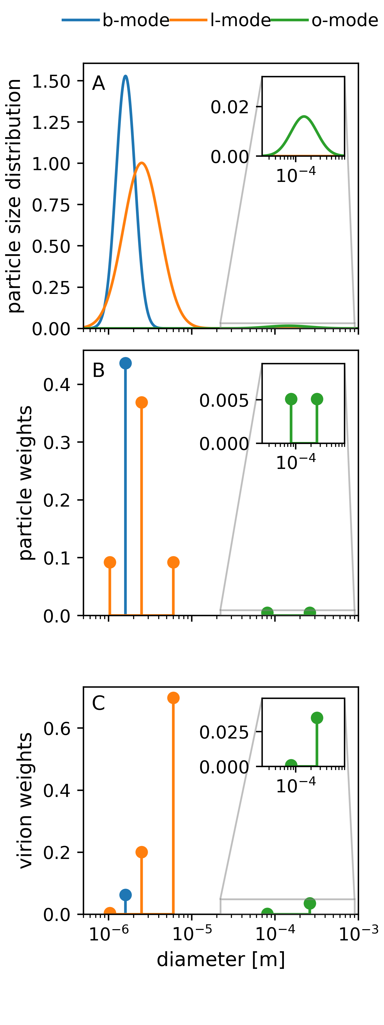
QuaRAD uses numerical quadrature to obtain an accurate and efficient representation of the size distribution of expelled aerosol particles and droplets. To construct the quadrature approximation, we follow the approach of Johnson et al., (2011) and represent expired particles through three different mechanisms, resulting in three lognormal distributions. Breath and speech create near continuous flows of small aerosol particles through the bronchial fluid film burst (BFFB) mechanism, the process of thin mucus films rupturing as the alveoli open and close deep in the lung (referred to as bronchial or b-mode particles); activities that vibrate the vocal cords further create slightly larger particles through laryngeal vibrations (referred to as laryngeal or l-mode particles); and expulsion of mucus from the mouth or nose generates the largest particles (referred to as oral or o-mode particles).
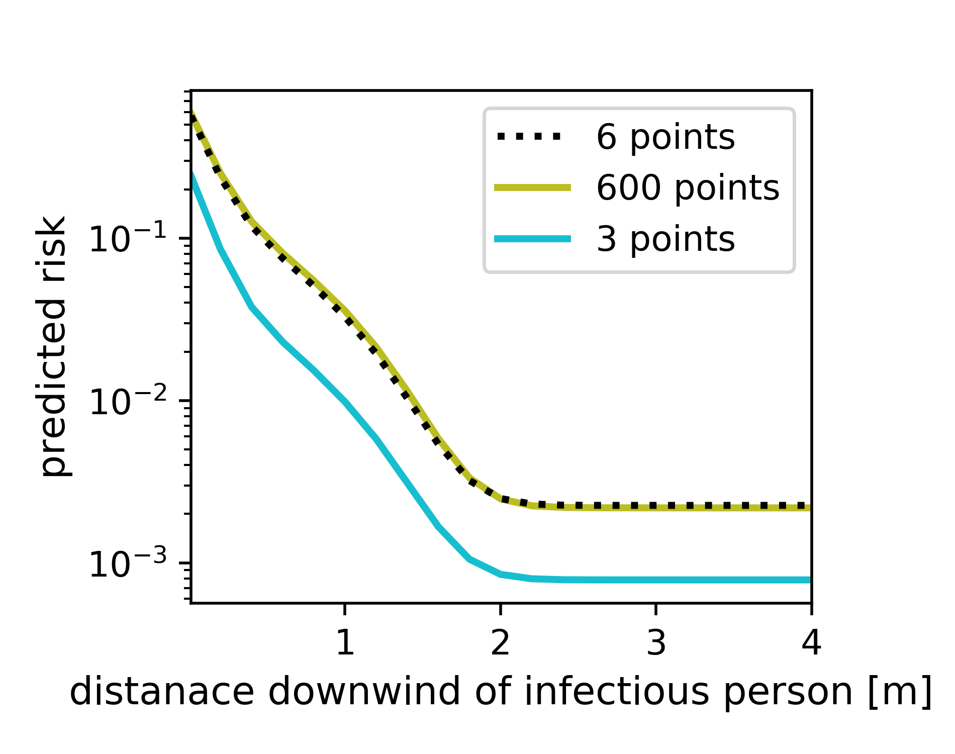
In QuaRAD, each of the three lognormal distributions is approximated using Gauss-Hermite quadrature. We found that one-point, three-point, and two-point quadrature were sufficient for representing the b-, l-, and o-modes, respectively, such that the overall distribution is represented with only six weighted particles; adding additional particles did not improve simulation accuracy (see Appendix A.1).
Gauss-Hermite quadrature approximates integrals of the form ; with a change of variables, integrals over lognormal distributions can also be expressed in this form. The expected value of a function of the natural logarithm of the diameter, , over a continuous lognormal distribution is given by:
| (1) |
where is the natural logarithm of the geometric mean and is the natural logarithm of the geometric standard deviation, the parameters of the lognormal distribution. With the following change of variables:
| (2) |
the integral over the continuous distribution is estimated by a quadrature approximation of the form:
| (3) |
where the abscissas are the roots of the physicists’ Hermite polynomial:
| (4) |
and the weights are given by:
| (5) |
The overall number concentration of virions, , is then given as the sum over , the number concentration of virions associated with each quadrature point:
| (6) |
The number of virions associated with a given quadrature point is computed as a function of the particle’s viral load — that is, the number of virions per volume of respiratory fluid — and its initial diameter:
| (7) |
where is the overall particle number concentration and is the viral load associated with quadrature point .
The distribution in virions with respect to particle size is an important parameter when modeling transmission, but the variation of SARS-CoV-2 loading within particles of different sizes has not yet been well quantified. A small number of studies have investigated virion expiration rates for other viruses with comparable viral loads (Jacot et al.,, 2020) in fine and coarse particles using the Gesundheit II (G-II), an instrument designed to capture and analyze respiratory particles (Milton et al.,, 2013; Leung et al.,, 2020). We combine the measurements of viral shedding from the G-II with the measurements of the particle size distributions by Johnson et al., (2011), Morawska et al., (2009), and Asadi et al., (2019) to estimate the viral load for particles in each mode. We assume that all virions in fine particles ( m) are distributed among the b- and l-mode particles and that virions in coarse particles ( m) are contained in o-mode particles; we assume the viral load is uniform across fine particles and across coarse particles. The weights corresponding to the distribution in virions, given by , are shown in Fig. 2c.
2.2 Water evaporation from particles
Expelled aerosol particles and droplets are predominantly water and contain small amounts of dissolved or suspended aerosol components, such as mucin, salts, and surfactants (Vejerano and Marr,, 2018). After they are expelled, water evaporates, causing the particles to shrink (Wei and Li,, 2015; Morawska et al.,, 2009), which may impact the distance a particle is able to travel before settling through sedimentation (Xie et al.,, 2007) and its deposition efficiency to nasal epithelium (Cheng,, 2003; Heyder,, 2004).
When first expelled, we assume particles are suspended in air that is saturated with water vapor () and at a temperature near the average human body temperature () (Wei and Li,, 2015). Following measurements by Vejerano and Marr, (2018), we assume that freshly expelled particles and droplets are 1%-9% dry aerosol by volume and that the aerosol mixture has an effective hygroscopicity parameter between 0.05 and 1. Once expelled, the particles cool and evaporate, with the rate of evaporation and equilibrium diameter dependent on the particles’ initial size, water content, and the hygroscopic properties of its aerosol constituents.
Following the approach of Kukkonen et al., (1989) and Wei and Li, (2015), we modeled evaporation by solving the following coupled set of ordinary differential equations:
| (8) | ||||
| (9) |
where is the mass of the aqueous particle, is the particle temperature, is the ambient pressure, is the vapor pressure at the droplet surface, is the vapor pressure far from the droplet surface, is the molecular weight of water, is the binary diffusion coefficient of water vapor in air far from the droplet surface, is the universal gas constant, is the specific heat of the particle, is the thermal conductivity of air, is the latent heat of vaporization, is a correction factor, Sh is the Sherwood number, and Nu is the Nusselt number. We assume spherical droplets to compute the diameter as a function of the mass of aerosol — assumed constant over the simulation — and water, which evolves according to Eqn. 8.
The evaporation model given in Eqn. 8 includes the enhancement in evaporation rate due to convection. This effect depends on the Sherwood number, the Nusselt number, and a correction factor for the diffusion coefficient due to the temperature difference between the particle and the air:
| (10) |
where is a constant between and , fixed at in this study. The Sherwood number is given by:
| (11) |
where Sc is the Schmidt number, given by:
| (12) |
where is the dynamic viscosity. The Nusselt number is given by:
| (13) |
where Pr is the Prandtl number, given by:
| (14) |
The rate at which an aqueous droplet evaporates is driven by the difference between the vapor pressure over the droplet and the vapor pressure of the ambient air, where droplet vapor pressures much larger than the ambient vapor pressure will result in rapid evaporation rates. We compute the vapor pressure over an aqueous particle using the Kappa-Köhler model (Petters and Kreidenweis,, 2007):
| (15) |
where is the saturation vapor pressure, is the particles’ dry diameter, is the effective hygroscopicity parameter of the aerosol contained in the particle, is the surface tension at the particle surface, and is the density of water. The vapor pressure over an aqueous droplet is computed relative to the saturation vapor pressure over a flat surface of pure water, which is computed as a function of the vapor temperature according to the Buck equation (Buck,, 1981):
| (16) |
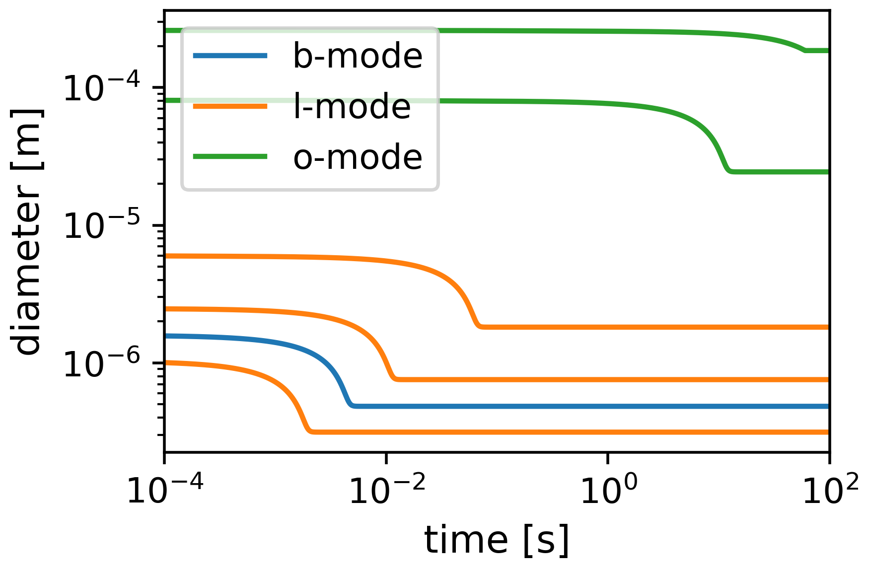
For the example scenario, the evolution of is shown in Fig. 3 for each quadrature point , upon exposure to the room-averaged temperature and relative humidity. All particles, regardless of their initial size, shrink over time, but the timescale for evaporation varies over orders of magnitude, as shown in previous studies (Morawska,, 2006; Redrow et al.,, 2011; Wei and Li,, 2015). The largest particles (o-mode, green) require more than ten seconds to reach their equilibrium size. On the other hand, the fine particles in the b-mode (blue) and l-mode (orange) reach equilibrium within to seconds, depending on their initial size. A particle’s diameter influences its transport through the expiratory jet, as described in the following section.
2.3 Particle dispersion within a turbulent jet
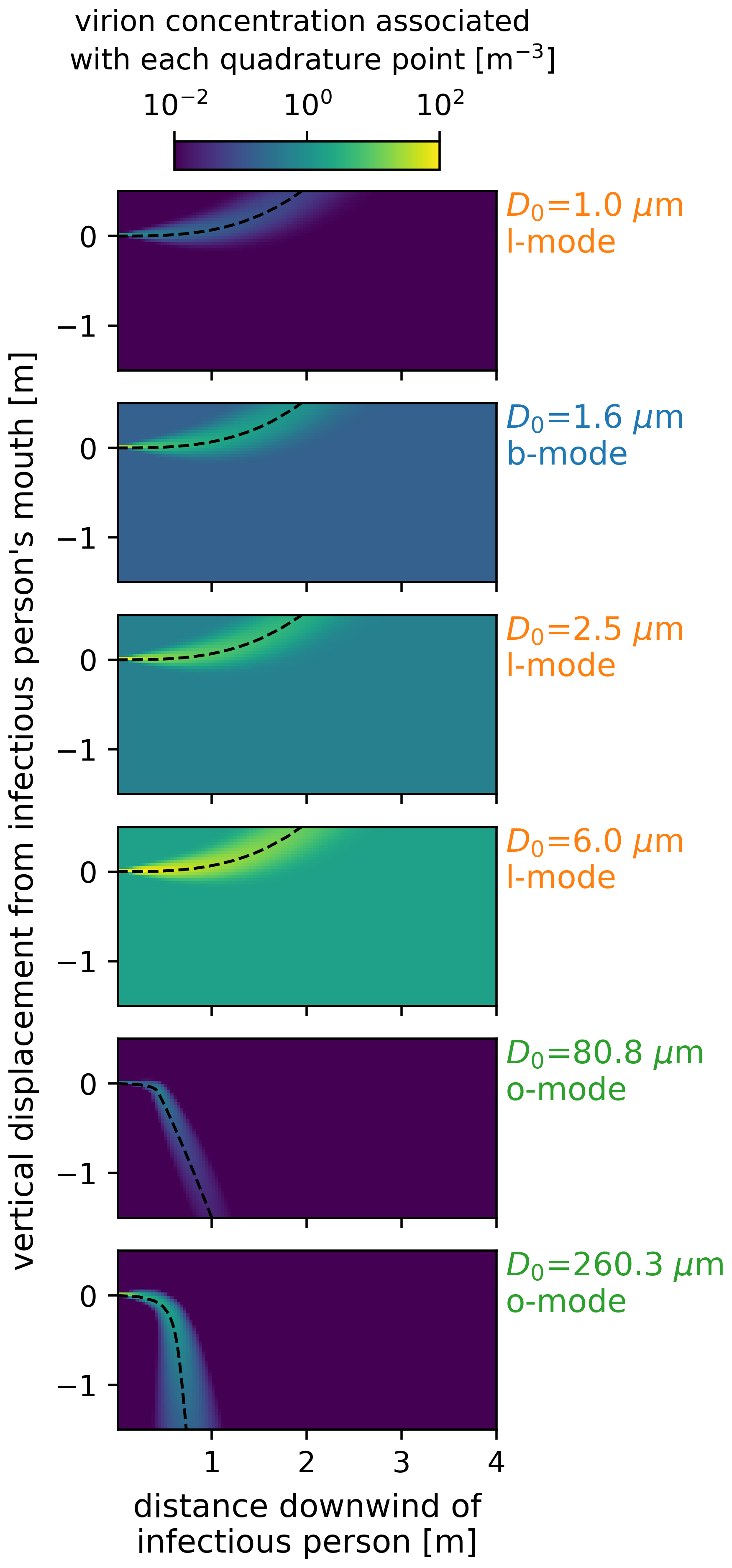
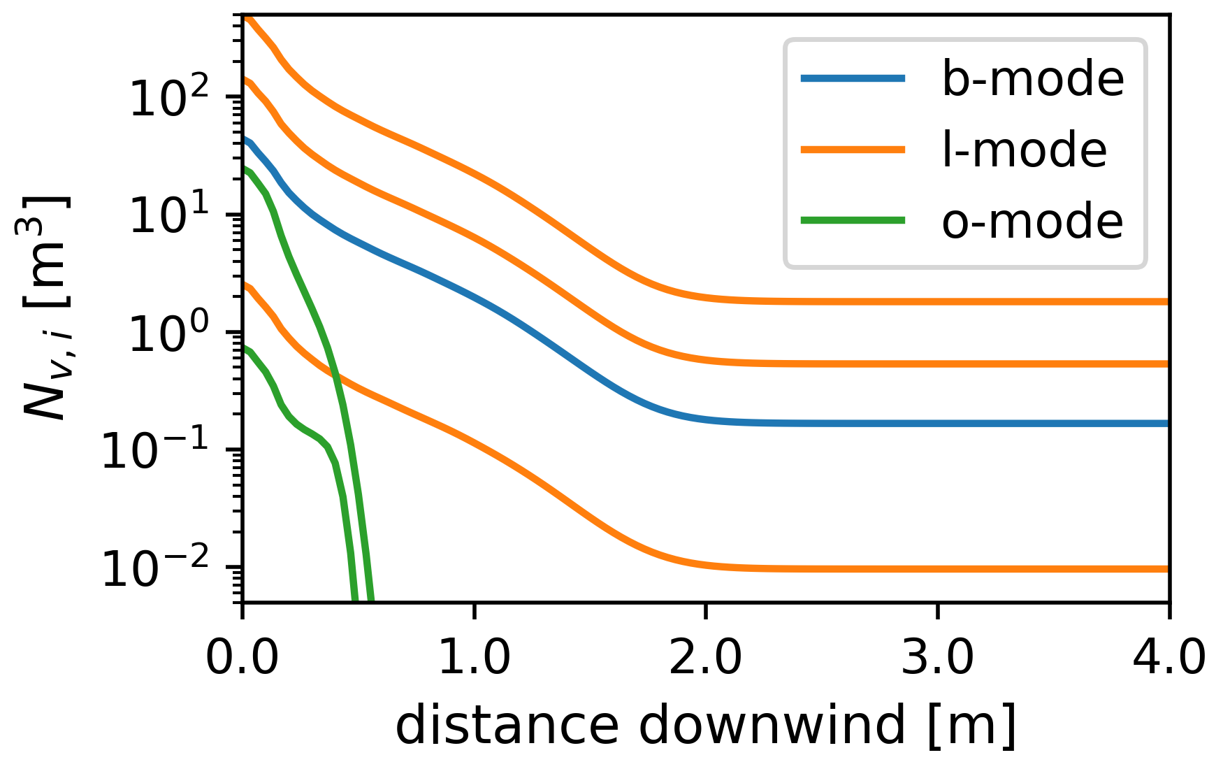
To predict the number concentration of virus-laden particles at a position , we represent the evolution of each quadrature point using the exposure model for indoor sources from Drivas et al., (1996). For an instantaneous source, such as a single cough, the concentration associated with each quadrature point is a function of position as well as time, denoted . A continuous emission source, such as talking, is represented as a series of puffs, such that the steady state concentration , as shown for each quadrature point in Fig. 4.
Following Drivas et al., (1996), we represent dispersion as the combination of a decay term and reflection terms , , and :
| (17) |
where ACH is the ventilation rate in air changes per hour, is the deposition velocity, is the deposition area, and is the room volume. The reflection terms in Drivas et al., (1996) account for reflections from the walls, floor, and ceiling, which are important for dispersion of gas-phase contaminants and small particles. We represent these wall reflections for particles smaller than m, and , , and are given by:
| (18) | |||
| (19) | |||
| (20) |
where , , and are the length, width, and height of the room, is the trajectory of a particle located in the center of the puff, and is the puff width. We assume that the infectious person is standing in the center of the room (,). In Eqns. 18–20, each infinite sum is replaced as the sum from -1000 to 1000, which was sufficient for convergence.
For particles larger than , we do not include reflections. The terms , , and are reduced to:
| (21) | |||
| (22) | |||
| (23) |
Whereas Drivas et al., (1996) represents exposure from the release of a toxin under quiescent conditions, we represent particle dispersion during talking using a turbulent jet model that includes buoyancy and gravitational settling. In the original formulation, , and are fixed at the location of the pollutant source. In contrast, we simulate the trajectory , , and within the expiratory jet of the infectious person. We assume that breadth of the puff is the same as the breadth of the jet, which is proportional to the distance traveled along the center line of the jet, :
| (25) |
To compute the position and velocity of a particle with diameter at the center of each puff, we follow the general approach of Wei and Li, (2015). The temporal evolution of particle position and velocity is determined by solving the set of six ordinary different equations that describe the motion of a particle in a moving gas (Crowe et al.,, 2011):
| (26) | |||
| (27) | |||
| (28) | |||
| (29) | |||
| (30) | |||
| (31) |
where , , and are the particle velocity in the -, -, and -directions, respectively, , , and are the gas velocity in the -, -, and -directions, respectively, is the drag coefficient, and is the acceleration due to gravity. The drag force is given by:
| (32) |
where Re is the Reynolds number. The Reynolds number for this case is given by:
| (33) |
where and . In this study, we represent cases with co-flow only, such that and . The gas velocity is predicted using the turbulent jet model of Lee et al., (2003) by modeling the infectious individual’s mouth as a circular orifice with diameter . Under this model, the co-flow velocity in the flow establishment zone () is given by:
| (34) |
where is the radial distance from the jet center line, b is the Gaussian half-width, and , where is the distance traveled along the jet center line. In the zone of established flow (), the velocity is given by:
| (35) |
The expelled air is typically warmer, moister, and contains more CO2 than the background air (Mahyuddin et al.,, 2014). The elevated temperature and water content cause the jet to curve upward due to buoyancy, which is partially offset by the increases in air density from the elevated concentration of CO2. We follow the approach of Baturin et al., (1972) to model the curve of the jet:
| (36) |
where is the source temperature, is the background temperature, and is the cross-sectional area of the jet orifice. The Archimedes number Ar0 is given by:
| (37) |
where is the difference between the background density, , and the source density, .
Similar to Xie et al., (2007) and Wei and Li, (2015), we use the relationships from Chen and Rodi, (1980) to represent the evolution in and the water vapor density within the turbulent jet. Once in the zone of established flow (), the center line temperature and the center line water vapor both decay with distance according to the same relationship:
| (38) |
In the flow establishment zone of the jet (), we assume that and .
The variation in and with the jet radius is then given by:
| (39) |
Water vapor is represented as an ideal gas, such that is computed from the partial pressure of water vapor :
| (40) |
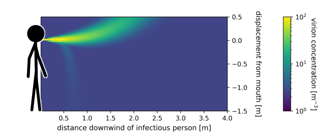
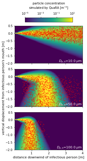
Using this combined jet dispersion model, we find that the spatial distribution in particles simulated by QuaRAD agrees well with the Discrete Random Walk (DRW) model of (Wei and Li,, 2015) (see comparison in Appendix A.2). Whereas the DRW model tracks thousands of Monte Carlo particles, QuaRAD simulates six quadrature points. The spatial distribution in virions associated with each QuaRAD point is shown in Fig. 7.
2.4 Virion exposure and risk of infection
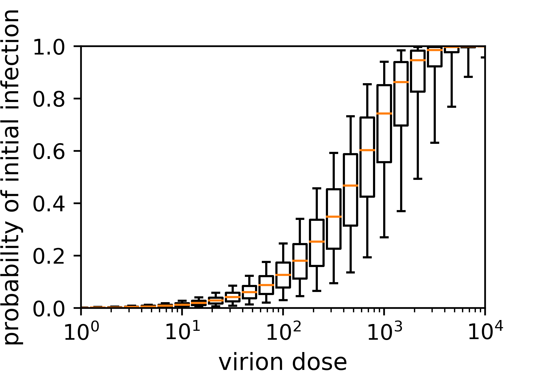
We applied the infection model described in Gale, (2020) to quantify the probability of initial SARS-CoV-2 infection as a function of the virion exposure level and host defense through the mucus barrier, such that the probability of infection increase with virion exposure and decreases with virion binding affinity to mucin molecules. The greater the number of virions to which a person is exposed, , the greater the number of chances that any given virion will successfully infect a cell. Differences in individuals’ immune responses are represented by modifying the probability that a virion infects a single cell, . The probability of initial infection within the host, , is then computed as a function of and :
| (41) |
To compute from the virion concentrations simulated in QuaRAD, we applied a respiratory deposition model to calculate the number of inhaled virions that reach the potential site of infection. In the case of SARS-CoV-2, infection must begin with a virion binding to an angiotensin-converting enzyme 2, or ACE2, receptor (Lukassen et al.,, 2020; Perrotta et al.,, 2020). As ACE2 expression within the respiratory tract is highest in the nasal epithelium and this is the most likely site of initial infection (Hou et al.,, 2020; Matheson and Lehner,, 2020; Ziegler et al.,, 2020), we assume that is the total number of virions that deposit to this region. We applied the model from Cheng, (2003) to predict the deposition efficiency to the nasal epithelium as a function of particle size:
| (42) |
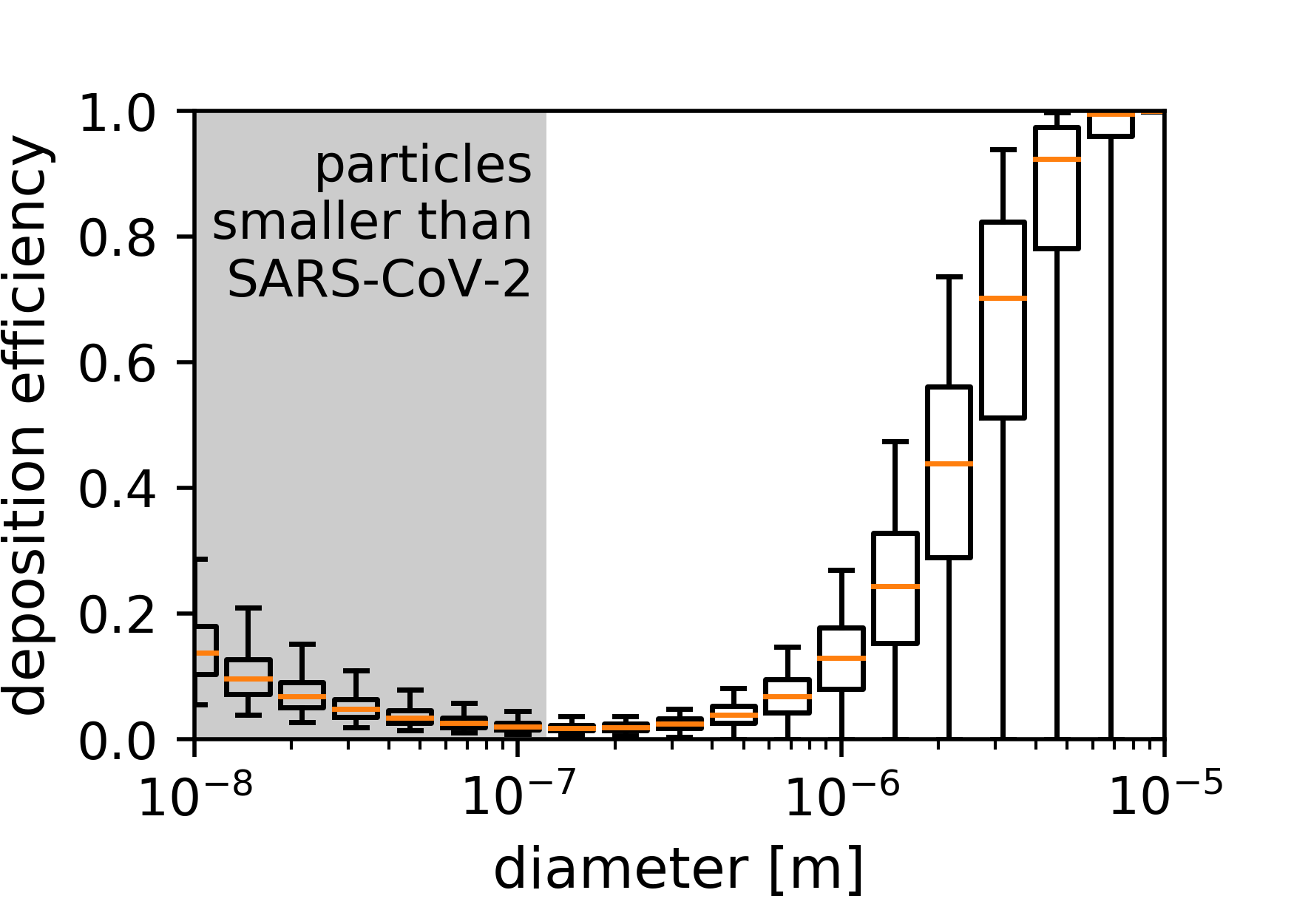
where is the aerodynamic diameter of the particle, is the molecular diffusion coefficient of the particle, is the breathing rate, and and are coefficients of deposition efficiency. We represent the uncertainty reported by Cheng, (2003) in the coefficients , , , and , leading to uncertainty in even for particles of the same size,. Fig. 5 shows the resulting variability in the size-dependent deposition represented across the ensemble of scenarios.
The overall rate at which virions deposit to the nasal epithelium, , is computed as the sum over the deposition rates associated with each of the quadrature points:
| (43) |
.
The probability that a virion infects a single cell, , is given by:
| (44) |
where is the fraction of virions that deposit to the infection site, is the fraction of virions at the infection site but not bound to the mucin, is the fraction of virions already bound to other cells, is the probability a given virion is capable of initiating an infection, and is the probability that a cell with a bound virus will become infected, defined as the virus successfully entering the cell, replicating, and releasing progeny virions. We assume that and based on Hoffmann et al., (2020) and Hui et al., (2020). We also assume that the only possible infection site is the nasal epithelium, and thus set for all virions depositing in this region. The fraction of ‘free’ virions not bound to the mucin, , is modeled as:
| (45) |
where is the association constant for binding of the virions to the mucin molecules and [] is the concentration of free mucin molecules remaining. These parameters likely vary widely among individuals, and the distributions in their values remains poorly constrained. Following the reasoning of Gale, (2020) and the measurements of Hou et al., (2020) and Kesimer et al., (2017), we assume that varies between 103 and 106 M-1 and that .
3 Results
We used QuaRAD to quantify the risk of airborne transmission of SARS-CoV-2 during a face-to-face encounter between an infectious and a susceptible person. Since a significant portion of SARS-CoV-2 transmission has been attributed to presymptomatic and asymptomatic carriers (Johansson et al.,, 2021; He et al.,, 2020; Byambasuren et al.,, 2020), who may transmit the virus before symptoms develop or may never develop symptoms, we focused on particles that are expelled when an infectious person is speaking. We quantified the risk of initial infection during a one-hour conversation as a function of distance between the infectious and the susceptible person, assuming that the infectious person is speaking continuously. To quantify uncertainty in transmission risk stemming from uncertainty in input parameters, we analyzed an ensemble of 10,000 simulations. First, we focus on an example scenario to illustrate how an infectious person influences virion concentrations within an indoor space.
3.1 Spatial variation in virion concentrations
A person shedding SARS-CoV-2 virions affects the average virion concentration in a room, but they have a far greater impact on virion concentrations in the region directly in front of them, as shown in Fig. 7. The overall concentration of virions, , is the sum over the concentration of virions associated with each quadrature point, for (see Fig. 4). Since this scenario represents a well-ventilated space (5 air changes per hour), the virion concentration far from the infectious person is relatively low (1 virion per m3). However, virion concentrations are orders of magnitude greater directly downwind of the infectious individual than in the rest of the room. A susceptible person standing in the expiratory jet of an infectious person will be exposed to a large concentration of virions, even if they are in a well-ventilated—or, in principle, unenclosed—space.
To identify the particle size ranges that are most important for virion transmission near and far from an infectious individual, we quantified the contribution of each quadrature point to the overall virion concentration, shown as a function of downwind distance (, ) in Fig. 8. Virions tend to be concentrated in the fine (b- and l-mode) particles rather than the coarse (o-mode) particles, regardless of the distance between the infectious and susceptible individual. In this scenario, the contribution of virions in o-mode particles drops to negligible values beyond 0.5 m from the infectious person, reflecting the general pattern that o-mode particles quickly fall to the ground. On the other hand, the long residence times of b- and l-mode particles allow them to affect virion concentrations elsewhere in the well-mixed room, albeit in lower concentrations than in the expiratory jet of an infectious person, and to persist much longer within the jet itself. This near-field enhancement in airborne transmission from these fine particles in the b- and l-modes extends much farther than the reach of the larger o-mode particles.
3.2 Near-field enhancement in the risk of airborne transmission
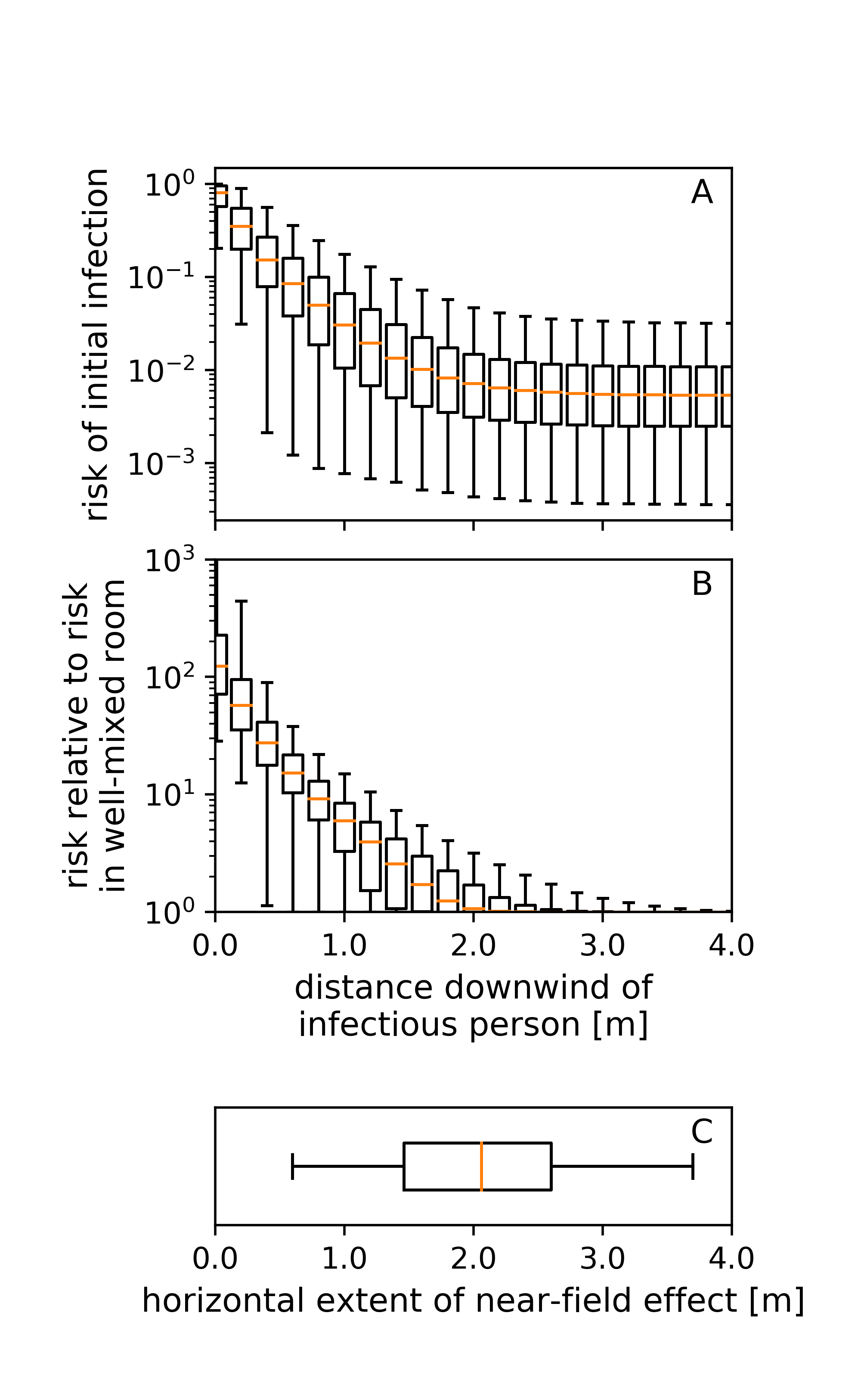
For the full ensemble of 10,000 simulations, the absolute risk of initial infection is shown as a function of distance downwind of an infectious person (, ) in Fig. 9a. The risk of an initial infection after an encounter with an infectious individual is orders of magnitudes higher when near the infectious individual than the average risk within the room. At any location, the risk of infection varies by over two orders of magnitude, due to the inherent variability in the parameters governing transmission. We caution that while this model is useful for comparing risk, predictions of absolute risk of initial infection (Fig. 9a) depend strongly on the assumed distribution in input parameters, many of which are poorly constrained.
At distances greater than three meters, the risk of initial infection by the susceptible person is equal to risk in a well-mixed room (assuming uniform concentration), whereas the risk of infection is orders of magnitude greater if the infectious and susceptible person are in a close, face-to-face conversation (0.5 m distancing). This enhancement in near-field risk is shown in Fig. 9b. Once the susceptible person moves beyond three meters from the infectious person, they avoid the near-field increases in virion concentrations and transmission is, thus, governed by the far-field concentration. These far-field concentrations are approximately the same as the concentration within a well-mixed room, reflected by values near unity for distances beyond three meters downwind in Fig. 9b.
3.3 Minimum distancing to avoid near-field enhancement in risk
To quantify the distance that one needs to remain from a potentially infectious person to avoid near-field enhancements in risk, we identified the distance at which the near-field impact drops below 5% of total transmission risk. Within this distance, local enhancements in virion concentrations increase transmission risk by more than 5%. We find that this threshold distance, , varies between one meter to four meters, suggesting large variability in near-field effects. In more than 50% of cases, we find is greater than the common recommendation of two meters (six feet).
To identify the model parameters that drive variability in , we applied the Delta Moment-Independent Measure (Borgonovo,, 2007) within the Sensitivity Analysis in Python (https://salib.readthedocs.io/en/latest/). The sensitivity index for each input parameter quantifies the fractional reduction in the variance of if the uncertainty in that parameter is eliminated. Across simulations, variability in is driven predominantly by variability in , the velocity at which particles are expelled, with a sensitivity index of 0.9. On the other hand, the most poorly constrained parameters, such as the rate of viral shedding and parameters governing the immune response in the new host, did not strongly affect variability in . Whereas the distribution in applied in this study represents an infectious person who is speaking at normal volume, the value of will be greater for a person who is sneezing, coughing, or speaking at a louder volume. For these events, we would then expect enhanced near-field transmission beyond the range of shown in Fig. 9c.
4 Conclusions
This paper describes the development the Quadrature-based model of Respiratory Aerosol and Droplets (QuaRAD) for simulating the evolution of respiratory particles and its application to simulate near-field transmission of airborne viruses. We showed that the risk of airborne transmission is elevated by orders of magnitude in the expiratory jet of the infectious person. The horizontal extent of this near-field increase in transmission risk was highly variable among simulations, and this variability was controlled by the velocity of the expired particles.
Since the risk of airborne transmission is strongly enhanced near infectious individuals, maintaining distance from those outside one’s household is a highly effective measure for reducing the spread of airborne pathogens. If a susceptible person moves far enough away, they can avoid the local increase in virion concentrations within the infectious person’s expiratory jet; at these long-range distances, the risk of infection is approximately the same as the risk within a well-mixed room. However, the simulations presented in this paper revealed that the elevated risk due to local increases in the virion concentration often extend beyond the typical two-meter (six-foot) distancing guidelines. These near-field impacts will extend even farther if the infectious person speaks loudly, sings, or even breathes heavily while exercising, as these activities expel particles at a higher velocities than conversational speech. On the other hand, if the infectious person is wearing a mask, they will expel particles at a slower velocity than if they are unmasked (Maher et al.,, 2020), reducing the horizontal extent of their near-field influence.
In general, we found tremendous variability of predicted transmission risk during any given encounter, due to the inherent variability in physiological properties of the infectious and susceptible individuals and in room conditions. To avoid the near-field enhancements in airborne exposure, distancing of at least three meters should be maintained. For situations in which distancing is not possible, such as interactions between healthcare workers and patients, it is important to provide protective equipment against airborne transmission, such as N95 respirators.
5 Data Availability
The QuaRAD source code, input files, and processing script are available for download at: https://github.com/lfierce2/QuaRAD/. Simulation ensembles were created using latin hypercube sampling with pyDOE: https://pythonhosted.org/pyDOE/. The sensitivity analysis was performed using the Sensitivity Analysis Library in Python, which is available at: https://salib.readthedocs.io/en/latest/.
6 Acknowledgements
This research was supported by the DOE Office of Science through the National Virtual Biotechnology Laboratory, a consortium of DOE national laboratories focused on response to COVID-19, with funding provided by the Coronavirus CARES Act. This project was supported in part by the U.S. Department of Energy through the Office of Science, Office of Workforce Development for Teachers and Scientists (WDTS) under the Science Undergraduate Laboratory Internships Program (SULI) and the Environmental and Climate Sciences Department under the BNL Supplemental Undergraduate Research Program (SURP). The quadrature-based model was originally developed for simulation of atmospheric aerosol with support from the DOE Atmospheric System Research program at Brookhaven National Laboratory, a multiprogram national laboratory supported by DOE Contract DE-SC0012704.
| Definition of Variables | ||
|---|---|---|
| variable | definition | units |
| surface area available for deposition | m2 | |
| cross-sectional area of the jet orifice | m2 | |
| ACH | air changes per hour | h-1 |
| Ar0 | Archimedes number | - |
| nasal deposition efficiency coefficients | - | |
| Gaussian half-width of jet | m | |
| drag coefficient | - | |
| concentration associated with quadrature point | particles/m3 | |
| specific heat of particle | J/(K kg) | |
| correction factor for diffusion coefficient | - | |
| initial particle diameter | m | |
| particle diameter | m | |
| particle aerodynamic diameter | m | |
| particle dry diameter | m | |
| molecular diffusion coefficient of particle | m | |
| diffusivity of water in air | ms | |
| diameter of infectious individual’s mouth | m | |
| deposition efficiency to nasal epithelium | - | |
| fraction of virions in exposure dose already | - | |
| bound to cells | ||
| fraction of virions in exposure dose transported | - | |
| to the infection site | ||
| fraction of virions in exposure dose not | - | |
| bound to mucin | ||
| fraction of virions residing in coarse particles | - | |
| acceleration due to gravity | m/s2 | |
| height of the room (-direction) | m | |
| quadrature abscissas | - | |
| Hermite polynomial | - | |
| average adult inhalation rate | breath/min | |
| average adult inhalation volume | m3/breath | |
| fresh air ventilation rate | s-1 | |
| thermal conductivity of air | W/(m K) | |
| association constant for binding between | M-1 | |
| virion and mucin | ||
| effective hygroscopicity parameter of aerosol | - | |
| contained in particle | ||
| length of the room (-direction) | m | |
| latent heat of vaporization | J/kg | |
| mass of aqueous particle p | kg | |
| molecular weight of water | kg/mol | |
| Geometric mean diameter of particles in the | m | |
| b-, l-, and o-mode, respectively | m | |
| concentration of free mucin molecules | molecules/mm3 | |
| particulate number emission rate for the b-, l-, | particles/s | |
| and o-mode, respectively | ||
| rate of virion deposition into the nasal epithelium | virions/s | |
| overall number concentration of particles | particles/m3 | |
| overall number concentration of virions | virions/m3 | |
| virions associated with quadrature point | virions/m3 | |
| Nu | the Nusselt number | - |
| dynamic viscosity | Pa s | |
| number emission rate of virions | virions/s | |
| ambient pressure | Pa | |
| probability that a single virion initiates an infection | - | |
| probability, given a bound virion, that a | ||
| cell becomes infected | ||
| probability of initial infection given an exposure dose | - | |
| probability that a given virion is capable of | - | |
| initiating infection in a cell | ||
| saturation vapor pressure of the air | Pa | |
| vapor pressure far from droplet surface | Pa | |
| vapor pressure at droplet surface | Pa | |
| Pr | the Prandtl number | - |
| radius of the jet’s potential core | m | |
| universal gas constant | J/(mol K) | |
| radial distance from the jet center line | m | |
| reflection terms in the -, -, and -directions, | - | |
| respectively | ||
| Re | the Reynolds number | - |
| RH | relative humidity | % |
| density of expired air | kg/m3 | |
| density of background air | kg/m3 | |
| density of aerosol in particle | kg/m3 | |
| density of gas | kg/m3 | |
| density of particle | kg/m3 | |
| center line water vapor density | kg/m3 | |
| density of water | kg/m3 | |
| initial plume saturation ratio | - | |
| background saturation ratio | - | |
| distance traveled along center line of the jet | m | |
| Sc | the Schmidt number | - |
| Sh | the Sherwood number | - |
| surface tension on particle surface | N/m | |
| geometric standard deviation of particle diameter | - | |
| in the b-, l-, and o-mode, respectively | - | |
| time | s | |
| initial plume temperature | K | |
| background temperature | K | |
| particle temperature | K | |
| vapor temperature | K | |
| centerline temperature | K | |
| initial expiration velocity | m/s | |
| gas velocity in the -direction | m/s | |
| particle velocity in the -direction | m/s | |
| room volume | m3 | |
| volumetric breathing rate | m3 / s | |
| number of virions in airborne exposure dose | virions | |
| bulk volume fraction of aerosol in droplet | mm3 | |
| gas velocity in the -direction | m/s | |
| viral load associated with quadrature point | virions/m3 | |
| particle velocity in the -direction | m/s | |
| width of the room (-direction) | m | |
| deposition rate onto surfaces | m/s | |
| gas velocity in the -direction | m/s | |
| weight associated with quadrature point | - | |
| particle velocity in the -direction | m/s | |
| location of source | m | |
| location of jet center line for each particle | m | |
| threshold distance at which local enhancement in virion | m | |
| concentration increases transmission risk by | ||
| location of source | m | |
| location of jet center line for each particle | m | |
| location of source (mouth height) | m | |
| location of jet center line for each particle | m | |
| variable | dist. |
min/mean/
geom. mean |
max/st. dev./
geom. st. dev |
nominal value | ref. |
|---|---|---|---|---|---|
| Expiration Parameters | |||||
| normal | |||||
| normal | 1 | ||||
| normal | |||||
| \hdashline | normal | 2 | |||
| normal | 3 | ||||
| Size Distribution Parameters | |||||
| normal | |||||
| normal | 4 | ||||
| normal | |||||
| \hdashline | normal | ||||
| normal | 4 | ||||
| normal | |||||
| \hdashline | normal | ||||
| normal | 4 | ||||
| normal | |||||
| Aerosol Parameters | |||||
| uniform | 5 | ||||
| uniform | 6 | ||||
| uniform | 7 | ||||
| \hdashline | lognormal | 8 | |||
| lognormal | |||||
| Room Parameters | |||||
| ACH | uniform | 9 | |||
| normal | 10 | ||||
| uniform | 11 | ||||
| normal | 12 | ||||
| \hdashline | uniform | 13 | |||
| uniform | |||||
| Inhalation & Deposition Parameters | |||||
| uniform | 14 | ||||
| uniform | 15 | ||||
| \hdashline | normal | ||||
| normal | 16 | ||||
| normal | |||||
| normal | |||||
| Infection Parameters | |||||
| normal | 17 | ||||
| \hdashline | lognormal | ||||
| uniform | 18 | ||||
| lognormal | |||||
Appendix A Appendix
A.1 Quadrature optimization
The size distribution of respiratory particles is represented in QuaRAD using a total of six quadrature points — 1-point, 3-point, and 2-point Gauss-Hermite quadrature for the b-, l-, and o-modes, respectively. We find that further increases in the number of quadrature points did not improve predictions; this is shown shown through comparison between the 6-point QuaRAD representation (blacked dashed line in Fig. A.1) and the same simulations but using 600 quadrature points (green line). On the other hand, if we use only one quadrature point for each of the b-, l-, and o-modes (teal line), we find the model accuracy decreases.
A.2 Verification against established Monte Carlo model
We verified particle dispersion simulated by QuaRAD through comparison with the Discrete Random Walk (DRW) model from Wei and Li, (2015). For each particle size, the DRW tracks the evolution of thousands of Monte Carlo particle. Instantaneous snap shots of particles simulated by DRW are compared with the steady-state solution from the jet-puff model (Section 2.3) in Fig. A.2. The top, middle, and center panels in Fig. A.2 show predictions for particles of diameter m, m, and m, respectively. In order to compare with the DRW simulations, evaporation and buoyancy were neglected in QuaRAD, and the particle expiration rate was adjusted to 33 particles per second. The steady-state concentration profiles simulated with QuaRAD agree with the DRW model (Fig. A.2), particularly in the cases of 10 m and 100 m particles; given the predominance of particles smaller than 10 m in the b- and l-modes and larger than 100 m in the o-mode, these sizes are the most relevant to the dispersion dynamics in QuaRAD.
References
- Antretter et al., (2010) Antretter, F., Holm, A., Karagiozis, A., and Glass, S. (2010). Interior temperature and relative humidity distributions in mixed-humid and cold climates as building simulation boundary conditions. In Proceedings: Thermal Performance of the Exterior Envelopes of Whole Buildings XI International Conference, Paper, volume 133.
- Asadi et al., (2019) Asadi, S., Wexler, A. S., Cappa, C. D., Barreda, S., Bouvier, N. M., and Ristenpart, W. D. (2019). Aerosol emission and superemission during human speech increase with voice loudness. Scientific reports, 9(1):1–10.
- Bahl et al., (2020) Bahl, P., Doolan, C., De Silva, C., Chughtai, A. A., Bourouiba, L., and MacIntyre, C. R. (2020). Airborne or droplet precautions for health workers treating covid-19? The Journal of infectious diseases.
- Baturin et al., (1972) Baturin, V. V. et al. (1972). Fundamentals of industrial ventilation. Pergamon Press Ltd Headington Hill Hall, Oxford.
- Beghein et al., (2005) Beghein, C., Jiang, Y., and Chen, Q. Y. (2005). Using large eddy simulation to study particle motions in a room. Indoor air, 15(4):281–290.
- Bennett et al., (2012) Bennett, D. H., Fisk, W., Apte, M. G., Wu, X., Trout, A., Faulkner, D., and Sullivan, D. (2012). Ventilation, temperature, and hvac characteristics in small and medium commercial buildings in california. Indoor air, 22(4):309–320.
- Bloch et al., (1985) Bloch, A. B., Orenstein, W. A., Ewing, W. M., Spain, W. H., Mallison, G. F., Herrmann, K. L., and Hinman, A. R. (1985). Measles outbreak in a pediatric practice: airborne transmission in an office setting. Pediatrics, 75(4):676–83.
- Borgonovo, (2007) Borgonovo, E. (2007). A new uncertainty importance measure. Reliability Engineering & System Safety, 92(6):771–784.
- Buck, (1981) Buck, A. L. (1981). New equations for computing vapor pressure and enhancement factor. Journal of Applied Meteorology and Climatology, 20(12):1527–1532.
- Byambasuren et al., (2020) Byambasuren, O., Cardona, M., Bell, K., Clark, J., McLaws, M.-L., and Glasziou, P. (2020). Estimating the extent of asymptomatic covid-19 and its potential for community transmission: systematic review and meta-analysis. Official Journal of the Association of Medical Microbiology and Infectious Disease Canada, 5(4):223–234.
- Chao et al., (2009) Chao, C. Y. H., Wan, M. P., Morawska, L., Johnson, G. R., Ristovski, Z., Hargreaves, M., Mengersen, K., Corbett, S., Li, Y., Xie, X., et al. (2009). Characterization of expiration air jets and droplet size distributions immediately at the mouth opening. Journal of aerosol science, 40(2):122–133.
- Chen and Rodi, (1980) Chen, C. J. and Rodi, W. (1980). Vertical turbulent buoyant jets: a review of experimental data. NASA Sti/Recon Technical Report A, 80:23073.
- Chen and Zheng, (2020) Chen, L. and Zheng, S. (2020). Understand variability of covid-19 through population and tissue variations in expression of sars-cov-2 host genes. Informatics in medicine unlocked, 21:100443.
- Chen et al., (2020) Chen, P. Z., Bobrovitz, N., Premji, Z., Koopmans, M., Fisman, D. N., and Gu, F. X. (2020). Heterogeneity in transmissibility and shedding sars-cov-2 via droplets and aerosols. medRxiv.
- Cheng, (2003) Cheng, Y. S. (2003). Aerosol deposition in the extrathoracic region. Aerosol Science & Technology, 37(8):659–671.
- Choi and Edwards, (2012) Choi, J.-I. and Edwards, J. R. (2012). Large-eddy simulation of human-induced contaminant transport in room compartments. Indoor air, 22(1):77–87.
- Crowe et al., (2011) Crowe, C. T., Schwarzkopf, J. D., Sommerfeld, M., and Tsuji, Y. (2011). Multiphase flows with droplets and particles. CRC press.
- Drivas et al., (1996) Drivas, P. J., Valberg, P. A., Murphy, B. L., and Wilson, R. (1996). Modeling indoor air exposure from short-term point source releases. Indoor Air, 6(4):271–277.
- Emmerich et al., (1994) Emmerich, S. J., Persily, A. K., and Walton, G. (1994). Application of a multi-zone airflow and contaminant dispersal model to indoor air quality control in residential buildings. NIST.
- EPA, (2018) EPA, U. (2018). Exposure factors handbook chapter 19 (update): Building characteristics. U.S. EPA Office of Research and Development.
- Fierce and McGraw, (2017) Fierce, L. and McGraw, R. L. (2017). Multivariate quadrature for representing cloud condensation nuclei activity of aerosol populations. Journal of Geophysical Research: Atmospheres, 122(18):9867–9878.
- Flenady et al., (2017) Flenady, T., Dwyer, T., and Applegarth, J. (2017). Accurate respiratory rates count: So should you! Australasian Emergency Nursing Journal, 20(1):45–47.
- Gale, (2020) Gale, P. (2020). Thermodynamic equilibrium dose-response models for mers-cov infection reveal a potential protective role of human lung mucus but not for sars-cov-2. Microbial risk analysis, 16:100140.
- GSA, (2019) GSA (2019). Space Planning. U.S. General Services Administration.
- He et al., (2020) He, X., Lau, E. H., Wu, P., Deng, X., Wang, J., Hao, X., Lau, Y. C., Wong, J. Y., Guan, Y., Tan, X., et al. (2020). Temporal dynamics in viral shedding and transmissibility of covid-19. Nature medicine, 26(5):672–675.
- Heyder, (2004) Heyder, J. (2004). Deposition of inhaled particles in the human respiratory tract and consequences for regional targeting in respiratory drug delivery. Proceedings of the American Thoracic Society, 1(4):315–320.
- Hoffmann et al., (2020) Hoffmann, M., Kleine-Weber, H., Schroeder, S., Krüger, N., Herrler, T., Erichsen, S., Schiergens, T. S., Herrler, G., Wu, N.-H., Nitsche, A., et al. (2020). Sars-cov-2 cell entry depends on ace2 and tmprss2 and is blocked by a clinically proven protease inhibitor. cell, 181(2):271–280.
- Hou et al., (2020) Hou, Y. J., Okuda, K., Edwards, C. E., Martinez, D. R., Asakura, T., Dinnon III, K. H., Kato, T., Lee, R. E., Yount, B. L., Mascenik, T. M., et al. (2020). Sars-cov-2 reverse genetics reveals a variable infection gradient in the respiratory tract. Cell, 182(2):429–446.
- Hui et al., (2020) Hui, K. P., Cheung, M.-C., Perera, R. A., Ng, K.-C., Bui, C. H., Ho, J. C., Ng, M. M., Kuok, D. I., Shih, K. C., Tsao, S.-W., et al. (2020). Tropism, replication competence, and innate immune responses of the coronavirus sars-cov-2 in human respiratory tract and conjunctiva: an analysis in ex-vivo and in-vitro cultures. The Lancet Respiratory Medicine, 8(7):687–695.
- Jacot et al., (2020) Jacot, D., Greub, G., Jaton, K., and Opota, O. (2020). Viral load of sars-cov-2 across patients and compared to other respiratory viruses. Microbes and infection, 22(10):617–621.
- Johansson et al., (2021) Johansson, M. A., Quandelacy, T. M., Kada, S., Prasad, P. V., Steele, M., Brooks, J. T., Slayton, R. B., Biggerstaff, M., and Butler, J. C. (2021). Sars-cov-2 transmission from people without covid-19 symptoms. JAMA network open, 4(1):e2035057–e2035057.
- Johnson et al., (2011) Johnson, G., Morawska, L., Ristovski, Z., Hargreaves, M., Mengersen, K., Chao, C. Y. H., Wan, M., Li, Y., Xie, X., Katoshevski, D., et al. (2011). Modality of human expired aerosol size distributions. Journal of Aerosol Science, 42(12):839–851.
- Kesimer et al., (2017) Kesimer, M., Ford, A. A., Ceppe, A., Radicioni, G., Cao, R., Davis, C. W., Doerschuk, C. M., Alexis, N. E., Anderson, W. H., Henderson, A. G., et al. (2017). Airway mucin concentration as a marker of chronic bronchitis. New England Journal of Medicine, 377(10):911–922.
- Kim et al., (2016) Kim, S.-H., Chang, S. Y., Sung, M., Park, J. H., Bin Kim, H., Lee, H., Choi, J.-P., Choi, W. S., and Min, J.-Y. (2016). Extensive viable middle east respiratory syndrome (mers) coronavirus contamination in air and surrounding environment in mers isolation wards. Reviews of Infectious Diseases, 63(3):363–369.
- Kukkonen et al., (1989) Kukkonen, J., Vesala, T., and Kulmala, M. (1989). The interdependence of evaporation and settling for airborne freely falling droplets. Journal of aerosol science, 20(7):749–763.
- Leclair et al., (1980) Leclair, J. M., Zaia, J. A., Levin, M. J., Congdon, R. G., and Goldmann, D. A. (1980). Airborne transmission of chickenpox in a hospital. New England Journal of Medicine, 302(8):450–453.
- Lee et al., (2003) Lee, J. H.-w., Chu, V., and Chu, V. H. (2003). Turbulent jets and plumes: A Lagrangian approach, volume 1. Springer Science & Business Media.
- Leung et al., (2020) Leung, N. H., Chu, D. K., Shiu, E. Y., Chan, K.-H., McDevitt, J. J., Hau, B. J., Yen, H.-L., Li, Y., Ip, D. K., Peiris, J. M., et al. (2020). Respiratory virus shedding in exhaled breath and efficacy of face masks. Nature medicine, 26(5):676–680.
- Li et al., (2005) Li, Y., Duan, S., Yu, I., and Wong, T. (2005). Multi-zone modeling of probable sars virus transmission by airflow between flats in block e, amoy gardens. Indoor air, 15(2):96–111.
- Lukassen et al., (2020) Lukassen, S., Chua, R. L., Trefzer, T., Kahn, N. C., Schneider, M. A., Muley, T., Winter, H., Meister, M., Veith, C., Boots, A. W., et al. (2020). Sars-cov-2 receptor ace 2 and tmprss 2 are primarily expressed in bronchial transient secretory cells. The EMBO journal, 39(10):e105114.
- Maher et al., (2020) Maher, B., Chavez, R., Tomaz, G. C., Nguyen, T., and Hassan, Y. (2020). A fluid mechanics explanation of the effectiveness of common materials for respiratory masks. International Journal of Infectious Diseases, 99:505–513.
- Mahyuddin et al., (2014) Mahyuddin, N., Awbi, H. B., and Alshitawi, M. (2014). The spatial distribution of carbon dioxide in rooms with particular application to classrooms. Indoor and Built Environment, 23(3):433–448.
- Matheson and Lehner, (2020) Matheson, N. J. and Lehner, P. J. (2020). How does sars-cov-2 cause covid-19? Science, 369(6503):510–511.
- McGraw, (1997) McGraw, R. (1997). Description of aerosol dynamics by the quadrature method of moments. Aerosol Science and Technology, 27(2):255–265.
- Meyerowitz et al., (2020) Meyerowitz, E. A., Richterman, A., Gandhi, R. T., and Sax, P. E. (2020). Transmission of sars-cov-2: a review of viral, host, and environmental factors. Annals of internal medicine.
- Milton et al., (2013) Milton, D. K., Fabian, M. P., Cowling, B. J., Grantham, M. L., and McDevitt, J. J. (2013). Influenza virus aerosols in human exhaled breath: particle size, culturability, and effect of surgical masks. PLoS pathogens, 9(3):e1003205.
- Morawska, (2006) Morawska, L. (2006). Droplet fate in indoor environments, or can we prevent the spread of infection? Indoor air, 16(5):335–347.
- Morawska et al., (2009) Morawska, L., Johnson, G., Ristovski, Z., Hargreaves, M., Mengersen, K., Corbett, S., Chao, C. Y. H., Li, Y., and Katoshevski, D. (2009). Size distribution and sites of origin of droplets expelled from the human respiratory tract during expiratory activities. Journal of Aerosol Science, 40(3):256–269.
- Morawska and Milton, (2020) Morawska, L. and Milton, D. K. (2020). It is time to address airborne transmission of coronavirus disease 2019 (covid-19). Clinical Infectious Diseases, 71(9):2311–2313.
- NCHS, (2021) NCHS (2021). Anthropometric reference data for children and adults: United states, 2015-2018. Analystical and Epidemiological Studies.
- Nguyen et al., (2014) Nguyen, J. L., Schwartz, J., and Dockery, D. W. (2014). The relationship between indoor and outdoor temperature, apparent temperature, relative humidity, and absolute humidity. Indoor air, 24(1):103–112.
- NYSDOH, (2010) NYSDOH (2010). Classroom Design Standards. New York State Department of Health Bureau of Emergency Medical Services.
- Perrotta et al., (2020) Perrotta, F., Matera, M. G., Cazzola, M., and Bianco, A. (2020). Severe respiratory sars-cov2 infection: Does ace2 receptor matter? Respiratory medicine, page 105996.
- Petters and Kreidenweis, (2007) Petters, M. and Kreidenweis, S. (2007). A single parameter representation of hygroscopic growth and cloud condensation nucleus activity. Atmospheric Chemistry and Physics, 7(8):1961–1971.
- Prather et al., (2020) Prather, K. A., Marr, L. C., Schooley, R. T., McDiarmid, M. A., Wilson, M. E., and Milton, D. K. (2020). Airborne transmission of sars-cov-2. Science, 370(6514):303–304.
- Redrow et al., (2011) Redrow, J., Mao, S., Celik, I., Posada, J. A., and Feng, Z.-g. (2011). Modeling the evaporation and dispersion of airborne sputum droplets expelled from a human cough. Building and Environment, 46(10):2042–2051.
- Riley et al., (1959) Riley, R. L., Mills, C., Nyka, W., Weinstock, N., Storey, P., Sultan, L., Riley, M., Wells, W., et al. (1959). Aerial dissemination of pulmonary tuberculosis. a two-year study of contagion in a tuberculosis ward. American Journal of Hygiene, 70(2):185–96.
- Samet et al., (2021) Samet, J. M., Prather, K., Benjamin, G., Lakdawala, S., Lowe, J.-M., Reingold, A., Volckens, J., and Marr, L. C. (2021). Airborne transmission of severe acute respiratory syndrome coronavirus 2 (sars-cov-2): What we know. Clinical Infectious Diseases.
- Sidebotham, (2007) Sidebotham, D. (2007). Cardiothoracic critical care. Elsevier Health Sciences.
- Stadnytskyi et al., (2020) Stadnytskyi, V., Bax, C. E., Bax, A., and Anfinrud, P. (2020). The airborne lifetime of small speech droplets and their potential importance in sars-cov-2 transmission. Proceedings of the National Academy of Sciences, 117(22):11875–11877.
- Tang et al., (2013) Tang, J. W., Nicolle, A. D., Klettner, C. A., Pantelic, J., Wang, L., Suhaimi, A. B., Tan, A. Y., Ong, G. W., Su, R., Sekhar, C., et al. (2013). Airflow dynamics of human jets: sneezing and breathing-potential sources of infectious aerosols. PloS one, 8(4):e59970.
- Turk et al., (1987) Turk, B., Brown, J., Geisling-Sobotka, K., Froehlich, D., Grimsrud, D., Harrison, J., Koonce, J., Prill, R., and Revzan, K. (1987). Indoor air quality and ventilation measurements in 38 pacific northwest commercial buildings. volume 1: Measurement results and interpretation. Lawrence Berkeley National Laboratory.
- Vejerano and Marr, (2018) Vejerano, E. P. and Marr, L. C. (2018). Physico-chemical characteristics of evaporating respiratory fluid droplets. Journal of The Royal Society Interface, 15(139):20170939.
- Watanabe et al., (2010) Watanabe, T., Bartrand, T. A., Weir, M. H., Omura, T., and Haas, C. N. (2010). Development of a dose-response model for sars coronavirus. Risk Analysis: An International Journal, 30(7):1129–1138.
- Wei and Li, (2015) Wei, J. and Li, Y. (2015). Enhanced spread of expiratory droplets by turbulence in a cough jet. Building and Environment, 93:86–96.
- Xie et al., (2007) Xie, X., Li, Y., Chwang, A., Ho, P., and Seto, W. (2007). How far droplets can move in indoor environments-revisiting the wells evaporation-falling curve. Indoor air, 17(3):211–225.
- Yu et al., (2004) Yu, I. T., Li, Y., Wong, T. W., Tam, W., Chan, A. T., Lee, J. H., Leung, D. Y., and Ho, T. (2004). Evidence of airborne transmission of the severe acute respiratory syndrome virus. New England Journal of Medicine, 350(17):1731–1739.
- Zhao et al., (2019) Zhao, X., Nie, W., Zhou, C., Cheng, M., Wang, C., Liu, Y., Li, J., Qian, Y., Ma, X., Zhang, L., et al. (2019). Airborne transmission of influenza virus in a hospital of qinhuangdao during 2017–2018 flu season. Food and environmental virology, 11(4):427–439.
- Ziegler et al., (2020) Ziegler, C. G., Allon, S. J., Nyquist, S. K., Mbano, I. M., Miao, V. N., Tzouanas, C. N., Cao, Y., Yousif, A. S., Bals, J., Hauser, B. M., et al. (2020). Sars-cov-2 receptor ace2 is an interferon-stimulated gene in human airway epithelial cells and is detected in specific cell subsets across tissues. Cell, 181(5):1016–1035.