A Detector-oblivious Multi-arm Network for Keypoint Matching
This is an extract from a complete paper, so if there existing contextual errors in the content, please ignore them. 9pt

Abstract

This paper presents a matching network to establish point correspondence between images. We propose a Multi-Arm Network (MAN) to learn region overlap and depth, which can greatly improve the keypoint matching robustness while bringing little computational cost during the inference stage. Another design that makes this framework different from many existing learning based pipelines that require re-training when a different keypoint detector is adopted, our network can directly work with different keypoint detectors without such a time-consuming re-training process. Comprehensive experiments conducted on outdoor and indoor datasets demonstrated that our proposed MAN outperforms state-of-the-art methods. Code will be made publicly available.

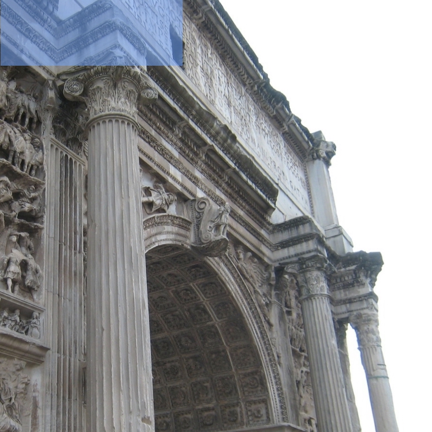
(a) A pair of images to be matched

(the blue masks cover the coarse overlap regions)

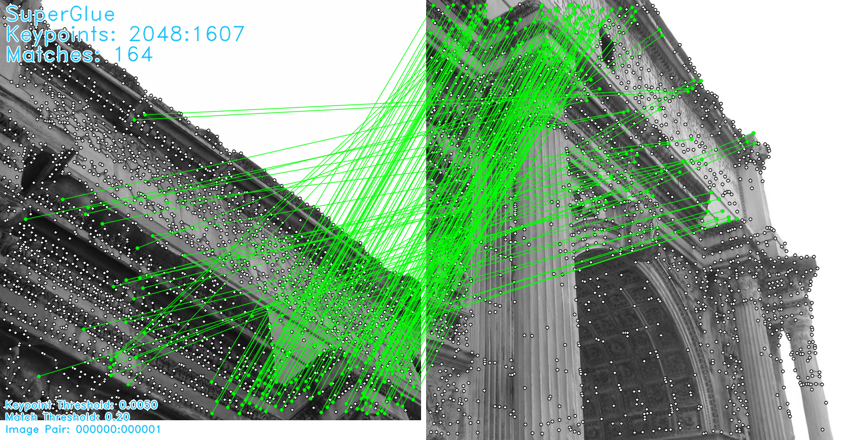
(b) The output from SuperGlue [9]

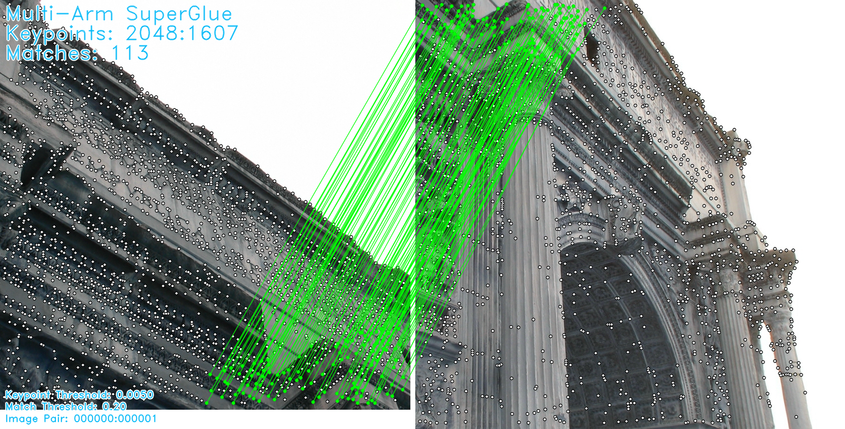
(c) The output from the MAN

Figure 1: (a). Humans tend to find coarse overlap regions in keypoint matching. (b)(c). We lead the MAN to aware of coarse overlap regions for each keypoints and tend to avoid match keypoints out of this region. In such challenging conditions, our proposed MAN finds more consistent correspondences than SuperGlue.

1 Introduction

Finding point correspondence is a fundamental problem in Computer Vision and has many important applications in visual Simultaneous Localization and Mapping (SLAM), Structure-from-Motion (SfM), and so on. Such correspondence is often solved through matching local features under certain geometric constraints (e.g., mutual nearest and ratio tests). Specifically, matching algorithms calculate similarities between a keypoint of an image and all the keypoints on another image.

In this work, our main idea is to mimic the human’s visual system. We expect the matching network to be aware of region-level information after communicating cross images. To this end, we propose to compute keypoint matching combine with solving two auxiliary tasks, with which region overlap and regional-level correspondence would have been estimated. Specifically, as the network estimates a feature for each keypoint, we expect this feature could contain the overlap region and depth region information of the keypoint. Fig. 1 illustrates this idea, whose difference from the current state-of-the-art matching approach (e.g., SuperGlue [9] is demonstrated).

SuperGlue [9] demonstrates remarkable performance in both outdoor and indoor datasets for keypoint matching. However, it needs to be fed with keypoint coordinates, descriptions, and confidence; hence it needs to be retrained each time when it adapts to different keypoint detectors. This training process will take a half month or more, even on the latest graphics cards. After conducting experiments on the influence of three keypoint attribution on SuperGlue, we find that the keypoint confidence has little effect on performance. Hence, we hypothesize that the keypoint confidence contributes little to the matching results. This discovery provides us with experimental support for removing keypoint confidence, and it is an important step in proposing the detector-oblivious network. We introduce a new design into the matching pipeline, the detector-oblivious description network, which is fed with keypoint coordinates from any detectors and outputs unique keypoint descriptions for it. With this design, our pipeline does not need to be retrained when a new detector is adopted.

In summary, our contributions are threefold:

• We propose a Multi-Arm Network (MAN) for keypoint matching, which utilizes region overlap and regional-level correspondence to enhance the robustness of keypoint matching.

• We develop a detector-oblivious description network that makes the matching pipeline be able to adapt to any keypoint detector without a time-consuming re-training procedure.

• We conduct thorough experiments and demonstrated that our pipeline leads to state-of-the-art results on both outdoor and indoor datasets.

2 Method

In this section, we will introduce our detector-oblivious multi-arm network for keypoint matching. Sec. 2.1 gives the problem formulation about keypoint matching. Sec. 2.2 introduces the approach to building the detector-oblivious network. Sec. LABEL:sec:MAN introduces the auxiliary tasks and loss functions developed in the multi-arm network for overlap and depth region estimation.

2.1 Problem formulation

Given a pair of images $\mathbf{A}$ and $\mathbf{B}$, each with a set of keypoint coordinates $\mathbf{p}$, which consist of $\mathbf{x}$ and $\mathbf{y}$ coordinates, $\mathbf{p}_{i}:=(\mathbf{x},\mathbf{y})_{i}$. Images $\mathbf{A}$ and $\mathbf{B}$ have $M$ and $N$ keypoint coordinates, indexed by $\mathcal{A}:=\{1,\ldots,M\}$ and $\mathcal{B}:=\{1,\ldots,N\}$, respectively. Our goal is to train a network that estimates the augmented partial assignment matrix, $\bar{\mathbf{P}}\in[0,1]^{\scaleto{(M+1)}{5pt}\times\scaleto{(N+1)}{5pt}}$, from two sets of keypoint coordinates.

2.2 Detector-oblivious approach

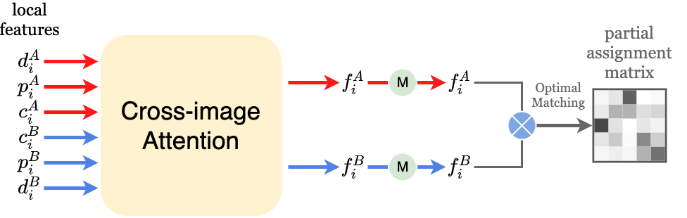
As illustrated in Fig. 2, SuperGlue requires input with keypoint descriptions $\mathbf{d}$, coordinates $\mathbf{p}$, and confidence $\mathbf{c}$, which represent as local features. Descriptions $\mathbf{d}_{i}\in\mathbb{R}^{D}$ and confidence $\mathbf{c}\in[0,1]$ can be extracted by a network, e.g., SuperPoint [2] and R2D2 [8], or an algorithm, e.g., SIFT [6].

However, if we train SuperGlue under SuperPoint [2], then we integrate it with other detectors, e.g., R2D2 [8], the performance will be bad. As SuperPoint and R2D2 are trained under different network architectures and loss functions, they will give two completely different keypoint descriptions $\mathbf{d}$ and confidence $\mathbf{c}$ for the same keypoint. SuperGlue can only learn one of the detectors through training and cannot transfer to other detectors directly.

Figure 2: The architecture of the original SuperGlue [9]. The $\mathbf{d}$, $\mathbf{p}$, and $\mathbf{c}$ represent keypoint descriptions, coordinates, and confidence, respectively.

Out of curiosity about the impact of the three input parameters ($\mathbf{d}$, $\mathbf{p}$, and $\mathbf{c}$) on the performance, we conducted a series of experiments (details can be found in Section 3). We found that $\mathbf{p}$ and $\mathbf{d}$ make the main contribution to performance, while $\mathbf{c}$ has very little. Therefore, we came up with an idea, since $\mathbf{c}$ hardly contributes to performance, why don’t we remove it? As such, we remove it.

Furthermore, we propose a detector-oblivious description function $\mathop{\gamma}(\mathbf{I},\mathbf{p})$ to obtain the keypoint descriptions $\mathbf{d}$, who is fed with an image $\mathbf{I}\in\{\mathbf{A},\mathbf{B}\}$ and keypoint coordinates $\mathbf{p}$. In practice, we implement the function $\mathop{\gamma}$ by a network. As such, we could convert keypoint descriptions $\mathbf{d}$ from a required input parameter to the intermediate value of the network. The network is used to implement $\mathop{\gamma}$ could be any network that satisfies the formula $\mathbf{d}=\mathop{\gamma}(\mathbf{I},\mathbf{p})$. Simply put, if a network could provide dense feature maps for the input image $\mathbf{I}$, then it could be used to implement $\mathop{\gamma}$.

In this way, we could build a detector-oblivious network architecture; see Fig. LABEL:fig:man. This network only requires to be fed with the keypoint coordinates $\mathbf{p}$ and can adapt to any keypoint detector with only one training process.

# Outdoor p d c MegaDepth (868 image pairs) YFCC (4000 image pairs) @$5^{\circ}$ @$10^{\circ}$ @$20^{\circ}$ $\mathbf{P}$ $\mathbf{M}$ @$5^{\circ}$ @$10^{\circ}$ @$20^{\circ}$ $\mathbf{P}$ $\mathbf{M}$ 1 SP SP SP $39.90$ $52.49$ $63.07$ $\mathbf{92.88}$ $25.91$ $38.92$ $59.12$ $75.45$ $\mathbf{98.72}$ $23.57$ 2 R2D2 SP SP $20.90$ $30.98$ $40.82$ $87.09$ $\mathbf{28.21}$ $34.94$ $54.97$ $71.31$ $97.43$ $\mathbf{29.65}$ 3 SP R2D2 SP $0.00$ $0.14$ $0.45$ $1.01$ $0.52$ $0.00$ $0.00$ $0.00$ $0.11$ $0.03$ 4 SP SP R2D2 $37.02$ $49.68$ $60.30$ $92.35$ $22.89$ $38.83$ $\mathbf{59.43}$ $\mathbf{75.78}$ $98.53$ $23.28$ 5 SP SP RAND $\mathbf{40.18}$ $\mathbf{52.64}$ $\mathbf{63.21}$ $92.76$ $25.95$ $\mathbf{39.10}$ $59.29$ $75.56$ $98.57$ $23.87$ 6 SP SP ZERO $36.96$ $49.88$ $60.59$ $91.05$ $25.95$ $37.86$ $58.27$ $75.00$ $98.48$ $24.07$ 7 SP SP ONE $38.70$ $51.59$ $62.74$ $92.81$ $26.49$ $38.60$ $58.91$ $75.46$ $98.42$ $24.44$ 8 SIFT SIFT SIFT $-$ $-$ $-$ $-$ $-$ $30.49$ $51.29$ $69.72$ $-$ $-$ 9 SIFT SP SIFT $24.77$ $35.19$ $45.82$ $89.66$ $15.53$ $\mathbf{37.28}$ $\mathbf{55.47}$ $\mathbf{70.65}$ $\mathbf{95.60}$ $15.37$ 10 SIFT SP RAND $\mathbf{25.39}$ $\mathbf{36.35}$ $46.70$ $\mathbf{89.69}$ $\mathbf{18.34}$ $36.43$ $54.91$ $70.60$ $95.45$ $\mathbf{17.22}$ 11 SIFT SP ZERO $25.30$ $36.13$ $46.92$ $88.73$ $15.60$ $36.30$ $54.39$ $69.77$ $95.31$ $15.57$ 12 SIFT SP ONE $24.56$ $35.46$ $\mathbf{47.00}$ $89.63$ $15.71$ $36.36$ $54.79$ $70.38$ $95.26$ $15.79$

Table 1: Outdoor pose estimation. The first column represents the number of the experiments. The $\mathbf{p}$, $\mathbf{d}$, and $\mathbf{c}$ represent keypoint coordinates, descriptions, and confidence, respectively. The $\mathbf{P}$ and $\mathbf{M}$ represent matching precision and matching score, respectively. In the outdoor scene, we find that record #5, whose confidence is set randomly, achieves better results on pose estimation than record #1, which is the original SuperGlue.

# Indoor p d c ScanNet (1500 image pairs) SUN3D (14872 image pairs) @$5^{\circ}$ @$10^{\circ}$ @$20^{\circ}$ $\mathbf{P}$ $\mathbf{M}$ @$5^{\circ}$ @$10^{\circ}$ @$20^{\circ}$ $\mathbf{P}$ $\mathbf{M}$ 1 SP SP SP $\mathbf{16.45}$ $\mathbf{33.62}$ $\mathbf{51.96}$ $\mathbf{84.13}$ $31.68$ $7.08$ $18.05$ $33.88$ $87.07$ $44.96$ 2 R2D2 SP SP $4.66$ $12.81$ $24.00$ $68.53$ $16.33$ $3.87$ $11.13$ $23.74$ $83.23$ $34.37$ 3 SP R2D2 SP $0.00$ $0.00$ $0.00$ $0.60$ $0.01$ $0.00$ $0.00$ $0.02$ $0.83$ $0.02$ 4 SP SP R2D2 $16.04$ $33.35$ $51.69$ $83.83$ $\mathbf{31.87}$ $7.07$ $17.96$ $33.86$ $86.94$ $45.04$ 5 SP SP RAND $15.54$ $32.77$ $50.47$ $83.31$ $31.78$ $\mathbf{7.17}$ $\mathbf{18.24}$ $\mathbf{34.10}$ $86.78$ $\mathbf{45.20}$ 6 SP SP ZERO $15.23$ $31.33$ $49.23$ $84.07$ $31.41$ $6.89$ $17.54$ $33.31$ $\mathbf{87.11}$ $44.76$ 7 SP SP ONE $14.70$ $31.70$ $49.34$ $82.58$ $31.61$ $7.07$ $18.14$ $33.94$ $86.32$ $45.09$ 8 SIFT SIFT SIFT $6.71$ $15.70$ $28.67$ $74.20$ $9.8$ $-$ $-$ $-$ $-$ $-$ 9 SIFT SP SIFT $\mathbf{7.80}$ $\mathbf{19.50}$ $\mathbf{33.88}$ $\mathbf{76.95}$ $19.05$ $5.78$ $14.97$ $\mathbf{29.13}$ $\mathbf{85.83}$ $32.40$ 10 SIFT SP RAND $7.77$ $18.85$ $33.52$ $76.36$ $\mathbf{20.40}$ $\mathbf{5.92}$ $\mathbf{15.03}$ $29.05$ $85.40$ $\mathbf{33.97}$ 11 SIFT SP ZERO $6.74$ $17.57$ $31.15$ $75.69$ $18.15$ $5.39$ $14.41$ $28.42$ $85.68$ $32.04$ 12 SIFT SP ONE $7.35$ $18.89$ $33.75$ $75.62$ $19.67$ $5.63$ $14.78$ $28.73$ $84.99$ $32.95$

Table 2: Indoor pose estimation. In ScanNet, record #1 performs best on the pose estimation. While in SUN3D record #5 performs better, and its confidence is set randomly.

3 Experiments for the detector-oblivious
approach

This section tests the influence of keypoint coordinates $\mathbf{p}$, descriptions $\mathbf{d}$, and confidence $\mathbf{c}$ for keypoint matching in SuperGlue [9] in outdoor and indoor scenes.

Metrics: We follow previous works  [9, 14, 16] and report the area under the cumulative error curve (AUC) of the pose error at the thresholds ($5^{\circ}$,$10^{\circ}$,$20^{\circ}$). The pose error is the maximum of the angular errors in rotation and translation. Poses are computed by first estimating the essential matrix with OpenCV’s findEssentialMat and RANSAC [3, 7] with an inlier threshold of $1$ pixel divided by the focal length, followed by recoverPose. In addition, we also report the matching precision ($\mathbf{P}$) and the matching score ($\mathbf{M}$) [15], where a match is considered correct based on its epipolar distance. The epipolar correctness threshold is $5\cdot 10^{-4}$.

Baselines: The original SuperGlue is trained under SuperPoint (SP), which is record #1 in Table 1 and Table 2. To test the generalization of SuperGlue integrated with different detectors, we change $\mathbf{p}$, $\mathbf{d}$, and $\mathbf{c}$ from original SP to R2D2.

Implement details: The SuperGlue model be used in this experiment is the official release model, which needs feeding with keypoint coordinates($2$-dim), descriptions($256$-dim), and confidence($scalar$). To fit the description input dimension of $256$, we train a $256$-dim R2D2 [8] by its official release code (the original R2D2 output $128$-dim descriptions for the keypoints).

3.1 Outdoor scenes

Details: In the outdoor scenario, we use the MegaDepth [5] dataset and the YFCC100M dataset [12] for testing. The MegaDepth consisting of $196$ different scenes reconstructed from $1,070,468$ internet photos using COLMAP [10, 11]. We select eight challenge scenes (868 image pairs) for evaluation. The YFCC100M contains several touristic landmark images whose ground-truth poses were created by generating 3D reconstructions from a subset of the collections [4]. We select four scenes (4000 image pairs) for evaluation.

Conditions: In testing, images are resized so that their longest dimension is equal to $1600$ pixels. We detect $2048$ keypoints for both R2D2 and SuperPoint.

Results: As shown in Table 1, after changing the keypoint coordinates $\mathbf{p}$, see record #2, the performance of pose estimation is decreased larger than 18% in MegaDepth. While in YFCC, this phenomenon is alleviated, but the performance is still degraded.

After changing the keypoint descriptors $\mathbf{d}$, see record #3; in both datasets, the model is not working. Because SuperGlue is only trained under SuperPoint’s description, it cannot adapt to R2D2’s description.

After replacing keypoint confidence $\mathbf{c}$ from SuperPoint (SP) to R2D2, random numbers, zeros, and ones, see record #4 - #7, in two datasets, the performance variance is small. In addition, we obtain the best pose estimation result on the MegaDepth when setting the keypoint confidence randomly, rather than the original SuperPoint one.

3.2 Indoor scenes

Datasets: In the indoor scenario, we use the ScanNet [1] dataset and the SUN3D dataset [13]. The ScanNet dataset is a large-scale indoor dataset composed of monocular sequences with ground truth poses and depth images. We select $1500$ image pairs from the well-defined test sequences for evaluation. The SUN3D dataset comprises a series of indoor videos captured with a Kinect, with 3D reconstructions, and we use the $14872$ image pairs from the well-defined test sequences for evaluation.

Conditions: In testing, images are resized so that their longest dimension is equal to $640$ pixels. We detect $1024$ keypoints for both R2D2 and SuperPoint.

Results: As shown in Table 2, after changing keypoint coordinates $\mathbf{p}$, see record #2, the pose estimation performance degrades significantly in both ScanNet and SUN3D.

After changing keypoint descriptors $\mathbf{d}$, see record #3, in both ScanNet and SUN3D, the model is not working. This result is consistent with the experimental results in the outdoor scene; see Table 1.

After replacing keypoint confidence $\mathbf{c}$ from SuperPoint (SP) to R2D2, random numbers, zeros, and ones, see record #4 - #7, in both ScanNet and SUN3D, there is little change in performance. In addition, we obtain the best pose estimation result in the SUN3D when setting the keypoint confidence randomly, while in the ScanNet, the original one still performs better than others.

Discussion about the keypoint confidence: Base on the experiment results above, we could conclude that the $\mathbf{p}$ and $\mathbf{d}$ dominate the matching performance of SuperGlue. About $\mathbf{c}$, we cannot say that $\mathbf{c}$ is insignificant for matching, but currently, in the SuperGlue architecture, it does not contribute much to matching.

For this result, a very intuitive guess is that the confidence of the keypoints is initially used in the keypoint selection stage. In the matching stage, the keypoints have been selected, and all the keypoints are treated equally for the matching method or network; therefore, the confidence of the keypoints is not important at this time.

However, another situation in which the current SuperGlue does not use the information in the $\mathbf{c}$ appropriately. We could find a better approach to dig out the valuable information from $\mathbf{c}$, such as combining the confidence value with the final matching results for joint consideration and calculation. In this work, we chose to remove $\mathbf{c}$ when matching keypoints to achieve the purpose of detector-oblivious.

4 Conclusion

This work proposed a multi-arm network to extract information from overlap and depth regions in the images, which provides extra supervision signals for training. Solving the auxiliary tasks of OVerlap Estimation (OVE) and DEpth region Estimation (DEE) help significantly improve the keypoint matching performance while bringing the little computational cost in inference.

Besides, we designed the detector-oblivious description network and integrated it into the matching pipeline. This design makes our network can directly adapt to unlimited keypoint detectors without a time-consuming re-training process.

References

- [1] Angela Dai, Angel X. Chang, M. Savva, Maciej Halber, T. Funkhouser, and M. Nießner. Scannet: Richly-annotated 3d reconstructions of indoor scenes. 2017 IEEE Conference on Computer Vision and Pattern Recognition (CVPR), 2017.
- [2] Daniel DeTone, Tomasz Malisiewicz, and Andrew Rabinovich. Superpoint: Self-supervised interest point detection and description. 2018 IEEE/CVF Conference on Computer Vision and Pattern Recognition Workshops (CVPRW), 2018.
- [3] M. Fischler and R. Bolles. Random sample consensus: a paradigm for model fitting with applications to image analysis and automated cartography. Commun. ACM, 1981.
- [4] Jared Heinly, J. Schonberger, E. Dunn, and J. Frahm. Reconstructing the world* in six days *(as captured by the yahoo 100 million image dataset). In CVPR 2015, 2015.
- [5] Z. Li and Noah Snavely. Megadepth: Learning single-view depth prediction from internet photos. 2018 IEEE/CVF Conference on Computer Vision and Pattern Recognition, 2018.
- [6] G. LoweDavid. Distinctive image features from scale-invariant keypoints. International Journal of Computer Vision, 2004.
- [7] R. Raguram, J. Frahm, and M. Pollefeys. A comparative analysis of ransac techniques leading to adaptive real-time random sample consensus. In ECCV, 2008.
- [8] Jérôme Revaud, C. D. Souza, M. Humenberger, and Philippe Weinzaepfel. R2d2: Reliable and repeatable detector and descriptor. In Advances in Neural Information Processing Systems, 2019.
- [9] Paul-Edouard Sarlin, Daniel DeTone, Tomasz Malisiewicz, and Andrew Rabinovich. SuperGlue: Learning feature matching with graph neural networks. In CVPR, 2020.
- [10] Johannes L. Schönberger and J. Frahm. Structure-from-motion revisited. 2016 IEEE Conference on Computer Vision and Pattern Recognition (CVPR), 2016.
- [11] Johannes L. Schönberger, Enliang Zheng, J. Frahm, and M. Pollefeys. Pixelwise view selection for unstructured multi-view stereo. In ECCV, 2016.
- [12] B. Thomee, D. Shamma, G. Friedland, B. Elizalde, Karl Ni, D. Poland, D. Borth, and L. Li. Yfcc100m: the new data in multimedia research. Commun. ACM, 2016.
- [13] J. Xiao, Andrew Owens, and A. Torralba. Sun3d: A database of big spaces reconstructed using sfm and object labels. 2013 IEEE International Conference on Computer Vision, 2013.
- [14] K. Yi, Eduard Trulls, Y. Ono, Vincent Lepetit, M. Salzmann, and P. Fua. Learning to find good correspondences. 2018 IEEE/CVF Conference on Computer Vision and Pattern Recognition, 2018.
- [15] Kwang Moo Yi, Eduard Trulls, Vincent Lepetit, and Pascal Fua. Lift: Learned invariant feature transform. In European conference on computer vision, 2016.
- [16] Jiahui Zhang, Dawei Sun, Zixin Luo, A. Yao, L. Zhou, Tianwei Shen, Y. Chen, Long Quan, and H. Liao. Learning two-view correspondences and geometry using order-aware network. 2019 IEEE/CVF International Conference on Computer Vision (ICCV), 2019.