Some Combinatorial Problems in Power-law Graphs

Abstract

The power-law behavior is ubiquitous in a majority of real-world networks, and it was shown to have a strong effect on various combinatorial, structural, and dynamical properties of graphs. For example, it has been shown that in real-life power-law networks, both the matching number and the domination number are relatively smaller, compared with homogeneous graphs. In this paper, we study analytically several combinatorial problems for two power-law graphs with the same number of vertices, edges, and the same power exponent. For both graphs, we determine exactly or recursively their matching number, independence number, domination number, the number of maximum matchings, the number of maximum independent sets, and the number of minimum dominating sets. We show that power-law behavior itself cannot characterize the combinatorial properties of a heterogenous graph. Since the combinatorial properties studied here have found wide applications in different fields, such as structural controllability of complex networks, our work offers insight in the applications of these combinatorial problems in power-law graphs.

1 Introduction

Let $\mathcal{G}=(\mathcal{V},\mathcal{E})$ be a connected unweighted graph with vertex set $\mathcal{V}$ and edge set $\mathcal{E}$. A matching of graph $\mathcal{G}$ is a subset of edge set $\mathcal{E}$, where no two edges are incident to a common vertex. A matching of maximum cardinality is called a maximum matching. The matching number of graph $\mathcal{G}$ is the cardinality of a maximum matching. An independent set of a graph $\mathcal{G}$ is a subset $\mathcal{I}$ of vertex set $\mathcal{V}$, such that each pair of vertices in $\mathcal{I}$ is not adjacent in $\mathcal{G}$. A maximum independent set (MIS) is an independent set $\mathcal{I}$ with the largest cardinality. The cardinality of a MIS for graph $\mathcal{G}$ is called its independent number. Graph $\mathcal{G}$ is called a unique independence graph if it has a unique MIS [1]. A dominating set of a graph $\mathcal{G}$ is a subset $\mathcal{D}$ of vertex set $\mathcal{V}$, such that every vertex in $\mathcal{V}\setminus\mathcal{D}$ is connected to at least one vertex in set $\mathcal{D}$. A dominating set $\mathcal{D}$ is called a minimum dominating set (MDS) if it has the least cardinality. The cardinality of a MDS for graph $\mathcal{G}$ is called its domination number.

The aforementioned combinatorial problems have been applied to numerous aspects in various disciplines or practical areas. For example, the size and the number of maximum matchings have found applications in physics [2], chemistry [3], computer science [4]; the MIS problem is associated with many fundamental graph problems, being equivalent to the minimum vertex cover problem [5] in the same graph and the maximum clique problem in its complement graph [6], and has been widely used to collusion detection in voting pools [7] and wireless networking schedules [8]; while the MDS problem is closely related to multi-document summarization in sentence graphs [9], routing on ad hoc wireless networks [10], and controllability in protein interaction networks [11]. Of particular interest is the connection of maximum matchings and MDS to structural controllability of complex networks [12], in the contexts of vertex [13] and edge [14] dynamics, respectively.

In view of the intrinsic relevance in both theoretical and practical scenarios, the above combinatorial problems have received considerable attention from the scientific community of theoretical computer science, theoretical physics, discrete mathematics, among others. In the past decade, these problems have become very active and have been popular research objects. Many authors have devoted their efforts to developing algorithms for the problems associated with maximum matchings [15, 16, 17, 18, 19, 20], MISs [21, 22, 23], as well as MDSs [24, 25, 26, 27, 28]. Although scientists have made a concerted effort, solving these problems is an important challenge and often computationally difficult. For example, finding a MDS [29] or a MIS [30, 31] of a general graph is NP-hard; while enumerating maximum matchings, or MISs, or MDSs in a graph is more difficult, which is #P-complete even in a bipartite graph [32, 33]. Thus, it makes sense to construct or seek special graph classes for which these combinatorial problems can be exactly solved [4], in order to achieve a particular goal.

On the other hand, extensive empirical study [34] has uncovered that a majority of real-world networks are typically scale-free [35], characterized by a power-law distribution $P(k)\sim k^{-\gamma}$ ($2<\gamma\leq 3$) for their vertex degree. This nontrivial scale-free structure is a fundamental concept in the study of the emerging network sciences. Many previous studies have shown that the scale-free topology plays an important role in various structural [36], combinatorial [13, 19, 26, 27, 28], and dynamical [37, 38, 39] properties of a graph. In the context of combinatorial aspect, it has been shown that compared with non-scale-free graphs, in scale-free networks, both the matching number [13] and the number of maximum matchings [19] are significantly smaller. It is the same with the domination number and the number of MDSs [26, 27, 20]. In addition, scale-free architecture also strongly affects the MIS problem [40] and its related optimization algorithms [41]. As is well known, in addition to the scale-free topology, many real networks show simultaneously some other remarkable properties, e.g., self-similarity [42]. Thus, it is difficult to separate the role or effect of a specific structural property in the performance of a network. Then, an interesting question is raised naturally: whether the scale-free structure is a unique ingredient characterizing the above combinatorial problems in power-law graphs?

In this paper, we study several combinatorial problems in two self-similar scale-free networks with the same power exponent: one is fractal but not small-world [43], the other is small-world but not fractal [44]. For both graphs, by using the decimation technique based on their self-similarity, we determine exactly the matching number, the independence number, and the domination number. Moreover, we determine exactly or recursively the number of maximum matchings, the number of MISs, and the number of MDSs. We show that the two networks differ in the studied quantities, which implies that scale-free topology alone cannot determine the combinatorial properties of power-law graphs, including maximum matchings, MISs and MDSs. Moreover, our exact results are instrumental for testing heuristic or stochastic algorithms associated with related combinatorial problems.

2 Constructions and structural properties of self-similar scale-free networks

In this section, we give a brief introduction to constructions and their structural properties of two self-similar scale-free networks, with the same number of vertices, the same number of edges, and the same power exponent. One is fractal but not small-world [43], the other is small-world but not fractal [44].

2.1 Constructions and structural properties of fractal scale-free networks

We first introduce the fractal scale-free networks under consideration, which are generated by an iterative way. Let $\mathcal{G}_{n}$, $n\geq 0$, denote the fractal scale-free network after $n$ iterations. Then, $\mathcal{G}_{n}$ is constructed as follows: For $n=0$, $\mathcal{G}_{0}$ is the complete graph $\mathcal{K}_{2}$ with two vertices connected by an iterative edge. For $n\geq 1$, $\mathcal{G}_{n}$ is obtained from $\mathcal{G}_{n-1}$ by performing the following operation: replace each iterative edge by the connected cluster on the right-hand side (rhs) of the arrow in Fig. 1.

Figure 1: Construction method for the fractal scale-free networks. To obtain network of next iteration, each iterative edge $(v_{i},v_{j})$ of current iteration is replaced by two parallel paths of two iterative edges (solid lines) on the rhs of the arrow, with $v_{i}$ and $v_{j}$ being the end vertices of two paths, and then link the two new vertices other than $v_{i}$ and $v_{j}$ by a new non-iterative edge (dotted line).

Figure 2 illustrates the construction process of the first several iterations.

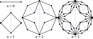
Figure 2: The first three iterations of the fractal scale-free networks.

The fractal scale-free networks are self-similar, which can be easily seen from an alternative construction approach [43] as shown in Fig. 3. For $\mathcal{G}_{n}$, $n\geq 0$, we call the two vertices in $\mathcal{G}_{0}$ as initial vertices, and denote them as $X_{n}$ and $Y_{n}$; while call the two vertices generated at iteration $1$ as hub vertices, and denote them as $W_{n}$ and $Z_{n}$. Then, given the network $\mathcal{G}_{n}$, $n\geq 1$, $\mathcal{G}_{n+1}$ can be obtained by merging four copies of $\mathcal{G}_{n}$ at their initial vertices. Let $\mathcal{G}_{n}^{(\theta)}$, $\theta=1,2,3,4$, be four replicas of $\mathcal{G}_{n}$, and denote the two initial vertices of $\mathcal{G}_{n}^{(\theta)}$ by $X_{n}^{(\theta)}$ and $Y_{n}^{(\theta)}$, respectively. Then, $\mathcal{G}_{n+1}$ can be obtained by merging $\mathcal{G}_{n}^{(\theta)}$, $\theta=1,2,3,4$, with $X_{n}^{(1)}$ ($Y_{n}^{(2)}$) and $X_{n}^{(3)}$ ($Y_{n}^{(4)}$) being identified as the initial vertex $X_{n+1}$ ($Y_{n+1}$) in $\mathcal{G}_{n+1}$, while $Y_{n}^{(1)}$ ($Y_{n}^{(3)}$) and $X_{n}^{(2)}$ ($X_{n}^{(4)}$) being identified as the hub vertex $W_{n+1}$ ($Z_{n+1}$) in $\mathcal{G}_{n+1}$. After the joining process, we link the two hub vertices $W_{n+1}$ and $Z_{n+1}$ by a non-iterative edge and get $\mathcal{G}_{n+1}$.

Figure 3: Second approach for the construction of $\mathcal{G}_{n+1}$.

Let $N_{n}$ and $E_{n}$, respectively, stand for the number of vertices and the number of edges in $\mathcal{G}_{n}$. By the second construction rules, $N_{n}$ and $E_{n}$ satisfy relations $N_{n}=4N_{n-1}-4$ and $E_{n}=4E_{n-1}+1$. With the initial conditions $N_{1}=4$ and $E_{1}=5$, we have $N_{n}=\frac{2}{3}\left(4^{n}+2\right)$ and $E_{n}=\frac{1}{3}\left(4^{n+1}-1\right)$. Then the average degree of all vertices in $\mathcal{G}_{n}$ is $\frac{2E_{n}}{N_{n}}=\frac{2(4^{n+1}-1)}{2\times 4^{n}+4}$, which is asymptotically equal to $4$ for large $n$.

The resulting graph $\mathcal{G}_{n}$ is scale-free, since the degree of its vertices obeys a power-law distribution $P(k)\propto k^{-3}$. Moreover, it is fractal with a fractal dimension being $2$ [43]. However, it is not small-world, since for large $n$, the average distance $\bar{d}_{n}$ of $\mathcal{G}_{n}$ grows as a power function of $N_{n}$, that is, $\bar{d}_{n}\sim(N_{n})^{1/2}$.

2.2 Constructions and structural properties of non-fractal scale-free networks

The second networks we consider are non-fractal and scale-free, which are also constructed iteratively. Let $\mathcal{G}^{\prime}_{n}$, $n\geq 0$, denote the network after $n$ iterations. Then, $\mathcal{G}^{\prime}_{n}$ is built as follows. For $n=0$, $\mathcal{G}^{\prime}_{0}$ is the complete graph $\mathcal{K}_{2}$ with two vertices connected by an iterative edge. For $n\geq 1$, $\mathcal{G}^{\prime}_{n}$ is obtained from $\mathcal{G}^{\prime}_{n-1}$ by performing the following operation: replace each iterative edge by the connected cluster on the rhs of the arrow in Fig. 4.

Figure 4: Construction method for the non-fractal scale-free networks. To obtain network of next iteration, each iterative edge $(v_{i},v_{j})$ of current iteration is replaced by two parallel paths of two iterative edges (solid lines) on the rhs of the arrow, with $v_{i}$ and $v_{j}$ being the end vertices of two paths, and then link $v_{i}$ and $v_{j}$ by a new non-iterative edge (dotted line).

Figure 5 illustrates the construction process of the first several iterations.

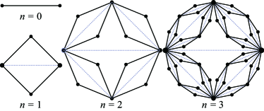
Figure 5: The first three iterations of the non-fractal scale-free networks.

The non-fractal scale-free network $\mathcal{G}^{\prime}_{n}$ is also self-similar, which suggests another construction approach highlighting its self-similarity [44] as shown in Fig. 6. For $\mathcal{G}^{\prime}_{n}$, $n\geq 0$, we call the two vertices in $\mathcal{G}^{\prime}_{0}$ as hub vertices, and denote them as $X^{\prime}_{n}$ and $Y^{\prime}_{n}$; while call the two vertices generated at iteration $1$ as border vertices, and denote them as $W^{\prime}_{n}$ and $Z^{\prime}_{n}$. Then, given the network $\mathcal{G}^{\prime}_{n}$, $n\geq 1$, $\mathcal{G}^{\prime}_{n+1}$ can be obtained by merging four copies of $\mathcal{G}^{\prime}_{n}$ at their hub vertices. Let $\mathcal{G}_{n}^{{}^{\prime}(\theta)}$, $\theta=1,2,3,4$, be four replicas of $\mathcal{G}^{\prime}_{n}$, and denote the two hub vertices of $\mathcal{G}_{n}^{{}^{\prime}(\theta)}$ by $X_{n}^{{}^{\prime}(\theta)}$ and $Y_{n}^{{}^{\prime}(\theta)}$, respectively. Then, $\mathcal{G}^{\prime}_{n+1}$ can be obtained by merging $\mathcal{G}_{n}^{{}^{\prime}(\theta)}$, $\theta=1,2,3,4$, with $X_{n}^{{}^{\prime}(1)}$ ($Y_{n}^{{}^{\prime}(2)}$) and $X_{n}^{{}^{\prime}(3)}$ ($Y_{n}^{{}^{\prime}(4)}$) being identified as the hub vertex $X^{\prime}_{n+1}$ ($Y^{\prime}_{n+1}$) in $\mathcal{G}^{\prime}_{n+1}$, while $Y_{n}^{{}^{\prime}(1)}$ ($Y_{n}^{{}^{\prime}(3)}$) and $X_{n}^{{}^{\prime}(2)}$ ($X_{n}^{{}^{\prime}(4)}$) being identified as the bounder vertex $W^{\prime}_{n+1}$ ($Z^{\prime}_{n+1}$) in $\mathcal{G}^{\prime}_{n+1}$. After the joining process, we link the two hub vertices $X^{\prime}_{n+1}$ and $Y^{\prime}_{n+1}$ by a non-iterative edge and get $\mathcal{G}^{\prime}_{n+1}$.

Figure 6: Second approach for the construction of $\mathcal{G}^{\prime}_{n+1}$.

By construction, $\mathcal{G}^{\prime}_{n}$ has the same number of vertices $N_{n}$, the same number of edge $E_{n}$, and thus the same average degree as those of $\mathcal{G}_{n}$. Moreover, the $\mathcal{G}^{\prime}_{n}$ is also scale-free with the same power exponent 3 as that of $\mathcal{G}_{n}$. However, different from $\mathcal{G}_{n}$, $\mathcal{G}^{\prime}_{n}$ is non-fractal since its fractal dimension is infinite, but is small-world, with its average distance average distance $\bar{d}_{n}$ growing logarithmically with the number of vertices $N_{n}$.

After introducing the construction and topological properties of the two self-similar scale-free networks, in what follows, by using their self-similarity we will study some combinatorial problems for these two networks, including the matching number, the independence number, the domination number, the number of maximum matchings, the number of MISs, and the number of MDSs. We will show that for the studied quantities, the two networks exhibit quite different behaviors. We note that in the process of the following computation or proof, we employ the same notation for $\mathcal{G}_{n}$ and $\mathcal{G}^{\prime}_{n}$ in the case without inducing confusion.

3 Matching number and the number of maximum matchings

In this section, we study the matching number and the number of maximum matchings in the self-similar scale-free networks.

3.1 Matching number and the number of maximum matchings in fractal scale-free networks

We first study the matching number and the number of maximum matchings in graph $\mathcal{G}_{n}$.

3.1.1 Matching number

Let $\beta_{n}$ denote the matching number of graph $\mathcal{G}_{n}$. In order to determine $\beta_{n}$, we define some intermediate quantities. Note that according to the number of covered initial vertices, all the matchings of $\mathcal{G}_{n}$ can be classified into three types: $\Omega^{0}_{n}$, $\Omega^{1}_{n}$ and $\Omega^{2}_{n}$, where $\Omega^{k}_{n}$, $k=0,1,2$, represent the set of matchings with each covering exactly $k$ initial vertices of $\mathcal{G}_{n}$. Let $\Theta^{k}_{n}$, $k=0,1,2$, be the subset of $\Omega^{k}_{n}$, where each matching has the largest cardinality, denoted by $\beta^{k}_{n}$, $k=0,1,2$. Then, $\beta_{n}={\rm max}\{\beta^{0}_{n},\beta^{1}_{n},\beta^{2}_{n}\}$.

Theorem 3.1.

The matching number of graph $\mathcal{G}_{n}$ is $\beta_{n}=\frac{4^{n}+2}{3}$.

Proof 3.2.

Since $\beta_{n}={\rm max}\{\beta^{0}_{n},\beta^{1}_{n},\beta^{2}_{n}\}$, we next evaluate the three quantities $\beta^{0}_{n}$, $\beta^{1}_{n}$ and $\beta^{2}_{n}$, all of which can be determined graphically.

Figures 7, 8, and 9 show, respectively, all the available configurations of maximum matchings of graph $\mathcal{G}_{n+1}$ belonging to $\Omega^{k}_{n+1}$, $k=0,1,2$, which contains all the matchings in $\Theta^{k}_{n+1}$. In Figs. 7, 8, and 9, only the initial vertices $X_{n}^{(\theta)}$ and $Y_{n}^{(\theta)}$ of $\mathcal{G}_{n}^{(\theta)}$, $\theta=1,2,3,4$, forming $\mathcal{G}_{n+1}$ are shown explicitly, with filled circles representing covered vertices and empty circles representing vacant vertices. Note that in Figs. 7, 8, and 9, if both of the hub vertices, $W_{n+1}$ and $Z_{n+1}$, of $\mathcal{G}_{n+1}$ are vacant, then the non-iterative edge connecting them is included in the matching in order to maximize its cardinality. From these three figures, we establish the following recursion relations for $\beta^{0}_{n}$, $\beta^{1}_{n}$, and $\beta^{2}_{n}$:

$$\beta^{0}_{n+1} ={\rm max}\{4\beta^{0}_{n}+1,3\beta^{0}_{n}+\beta^{1}_{n},2\beta^{0}_{n}+2\beta^{1}_{n}\}\,,$$ (1)

$$\beta^{1}_{n+1} ={\rm max}\{3\beta^{0}_{n}+\beta^{1}_{n}+1,3\beta^{0}_{n}+\beta^{2}_{n},2\beta^{0}_{n}+2\beta^{1}_{n},$$

$$\quad\quad\quad\quad 2\beta^{0}_{n}+\beta^{1}_{n}+\beta^{2}_{n},\beta^{0}_{n}+3\beta^{1}_{n}\}\,,$$ (2)

$$\beta^{2}_{n+1} ={\rm max}\{2\beta^{0}_{n}+2\beta^{1}_{n}+1,2\beta^{0}_{n}+\beta^{1}_{n}+\beta^{2}_{n},\beta^{0}_{n}+3\beta^{1}_{n},$$

$$\quad\quad\quad\quad 2\beta^{0}_{n}+2\beta^{2}_{n},\beta^{0}_{n}+2\beta^{1}_{n}+\beta^{2}_{n},4\beta^{1}_{n}\}\,.$$ (3)

With initial condition $\beta^{0}_{1}=1$, $\beta^{1}_{1}=1$, and $\beta^{2}_{1}=2$, the above equations are solved to yield $\beta^{0}_{n}=\frac{4^{n}-1}{3}$, $\beta^{1}_{n}=\frac{4^{n}-1}{3}$, and $\beta^{2}_{n}=\frac{4^{n}+2}{3}$.

Since the number of vertices $N_{n}$ in graph $\mathcal{G}_{n}$ is $N_{n}=\frac{2}{3}\left(4^{n}+2\right)$, which is exactly twice as large as the matching number $\beta_{n}=\frac{4^{n}+2}{3}$, there are perfect matchings in $\mathcal{G}_{n}$ for all $n\geq 0$.

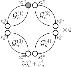
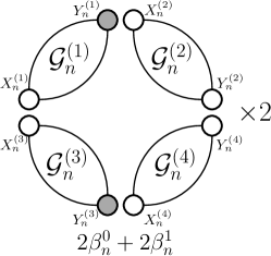
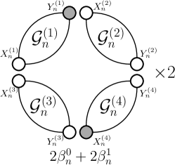
Figure 7: Illustration of all possible configurations and their sizes of matchings for graph $\mathcal{G}_{n+1}$ belonging to $\Omega^{0}_{n+1}$, which contain all matchings in $\Theta^{0}_{n+1}$.

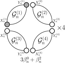
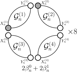
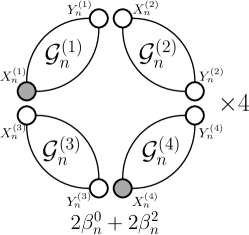
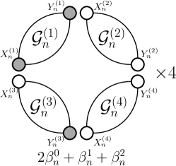
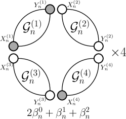
Figure 8: Illustration of all possible configurations and their sizes of matchings for graph $\mathcal{G}_{n+1}$ belonging to $\Omega^{1}_{n+1}$, which contain all matchings in $\Theta^{1}_{n+1}$.

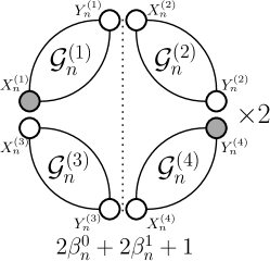
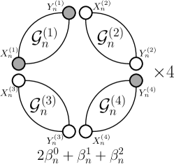
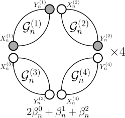
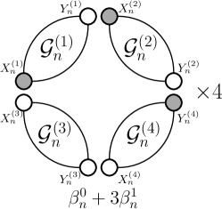
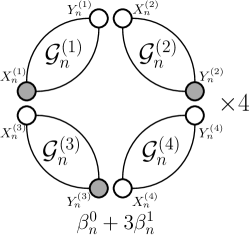
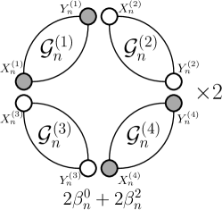
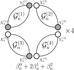
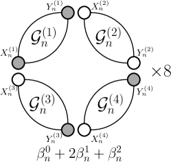
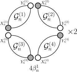
Figure 9: Illustration of all possible configurations and their sizes of matchings for graph $\mathcal{G}_{n+1}$ belonging to $\Omega^{2}_{n+1}$, which contain all matchings in $\Theta^{2}_{n+1}$.

3.1.2 Number of maximum matchings

Let $\theta_{n}$ denote the number of maximum matchings or perfect matchings in $\mathcal{G}_{n}$. To calculate $\theta_{n}$, we introduce an additional quantity $\phi_{n}$, which denotes the number of maximum matchings in $\Omega^{0}_{n}$, satisfying that each matching is maximum among all the matchings of $\mathcal{G}_{n}$ with both initial vertices $X_{n}$ and $Y_{n}$ being vacant.

Theorem 3.3.

The number of maximum matchings of $\mathcal{G}_{n}$, $n\geq 1$, is $2^{2^{n}-1}$.

Proof 3.4.

Note that for $n=1$, $\theta_{1}=2$ and $\phi_{1}=1$. For $n\geq 1$, we first establish the following recursion relations for the two quantities $\theta_{n}$ and $\phi_{n}$ associated with graph $\mathcal{G}_{n}$:

$$\theta_{n+1}= 2\theta_{n}^{2}\phi_{n}^{2},$$ (4)

$$\phi_{n+1}= \phi_{n}^{4}.$$ (5)

We only prove Eq. (5). Since $\beta^{0}_{n}=\beta^{1}_{n}$, Eq. (1) and Fig. 7 show that, the cardinality of each matching in $\Omega^{0}_{n+1}$ is maximized if and only if all the matchings of the four copies $\mathcal{G}_{n}^{(\theta)}$, $\theta=1,2,3,4$, are in $\Omega^{0}_{n}$. Then, we establish $\phi_{n+1}=\phi_{n}^{4}$.

By using Eq. (1) and Fig. 9, Eq. (4) can be proved analogously.

Equations (4) and (5), together with the initial conditions $\theta_{1}=2$ and $\phi_{1}=1$, are solved to yield $\theta_{n}=2^{2^{n}-1}$ and $\phi_{n}=1$ for all $n\geq 1$.

Note that both the matching number and the number of maximum matchings for graph $\mathcal{G}_{n}$ have been previously obtained in [19] by using the technique of Pfaffian orientations, which is more complicated than the approach used here.

3.2 Matching number and the number of maximum matchings in non-fractal scale-free networks

We continue to study the matching number and the number of maximum matchings in graph $\mathcal{G}^{\prime}_{n}$.

3.2.1 Matching number

Let $\Omega^{k}_{n}$, $k=0,1,2$, represent matchings covering exactly $k$ hub vertices of $\mathcal{G}^{\prime}_{n}$. Let $\Theta^{k}_{n}$, $k=0,1,2$, be the subset of $\Omega^{k}_{n}$, where each matching has the largest cardinality among all matchings in $\Omega^{k}_{n}$, with the largest cardinality being denoted by $\beta^{k}_{n}$, $k=0,1,2$. Then, the matching number $\beta_{n}$ of $\mathcal{G}^{\prime}_{n}$ can be expressed as $\beta_{n}={\rm max}\{\beta^{0}_{n},\beta^{1}_{n},\beta^{2}_{n}\}$.

Theorem 3.5.

The matching number of graph $\mathcal{G}^{\prime}_{n}$ is $\beta_{n}=\frac{2^{2n-1}+4}{3}$.

Proof 3.6.

In order to find $\beta_{n}$, we can alternatively evaluate the three quantities $\beta^{0}_{n}$, $\beta^{1}_{n}$ and $\beta^{2}_{n}$ by using the self-similar structure of graph $\mathcal{G}^{\prime}_{n}$. We now graphically compute $\beta^{k}_{n}$, $k=0,1,2$. Figures 10, 11, and 12 show, respectively, all the possible configurations of matchings in $\Omega^{0}_{n+1}$, $\Omega^{1}_{n+1}$ and $\Omega^{2}_{n+1}$, which contain $\Theta^{0}_{n+1}$, $\Theta^{1}_{n+1}$ and $\Theta^{2}_{n+1}$. In Figs. 10, 11, and 12, only the hub vertices $X_{n}^{{}^{\prime}(\theta)}$ and $Y_{n}^{{}^{\prime}(\theta)}$ of $\mathcal{G}_{n}^{{}^{\prime}(\theta)}$, $\theta=1,2,3,4$, forming $\mathcal{G}^{\prime}_{n+1}$ are shown explicitly, with filled circles denoting covered vertices and empty circles denoting vacant vertices. Note that in Fig. 12, the iterative edge linking the two hub vertices $X^{\prime}_{n+1}$ and $Y^{\prime}_{n+1}$ of $\mathcal{G}^{\prime}_{n+1}$ will be included in the matching if both of the two hub vertices of $\mathcal{G}^{\prime}_{n+1}$ are vacant after joining process. From Figs. 10, 11, and 12, we establish recursive relations governing $\beta^{0}_{n}$, $\beta^{1}_{n}$, and $\beta^{2}_{n}$:

$$\beta^{0}_{n+1} ={\rm max}\{4\beta^{0}_{n},3\beta^{0}_{n}+\beta^{1}_{n},2\beta^{0}_{n}+2\beta^{1}_{n}\}\,,$$ (6)

$$\beta^{1}_{n+1} ={\rm max}\{3\beta^{0}_{n}+\beta^{1}_{n},3\beta^{0}_{n}+\beta^{2}_{n},2\beta^{0}_{n}+2\beta^{1}_{n},$$

$$\quad\quad\quad\quad 2\beta^{0}_{n}+\beta^{1}_{n}+\beta^{2}_{n},\beta^{0}_{n}+3\beta^{1}_{n}\}\,,$$ (7)

$$\beta^{2}_{n+1} ={\rm max}\{2\beta^{0}_{n}+2\beta^{1}_{n},2\beta^{0}_{n}+\beta^{1}_{n}+\beta^{2}_{n},\beta^{0}_{n}+3\beta^{1}_{n},$$

$$\quad\quad\quad\quad 2\beta^{0}_{n}+2\beta^{2}_{n},\beta^{0}_{n}+2\beta^{1}_{n}+\beta^{2}_{n},4\beta^{1}_{n},4\beta^{0}_{n}+1,$$

$$\quad\quad\quad\quad 3\beta^{0}_{n}+\beta^{1}_{n}+1,2\beta^{0}_{n}+2\beta^{1}_{n}+1\}\,.$$ (8)

With initial condition $\beta^{0}_{1}=0$, $\beta^{0}_{1}=1$, and $\beta^{0}_{1}=2$, the above equations are solved to yield $\beta^{0}_{n}=\frac{2^{2n-1}-2}{3}$, $\beta^{1}_{n}=\frac{2^{2n-1}+1}{3}$, and $\beta^{2}_{n}=\frac{2^{2n-1}+4}{3}$.

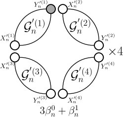
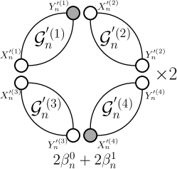
Figure 10: Illustration of all possible configurations and their sizes of matchings for graph $\mathcal{G}^{\prime}_{n+1}$ belonging to $\Omega^{0}_{n+1}$, which contain all matchings in $\Theta^{0}_{n+1}$.

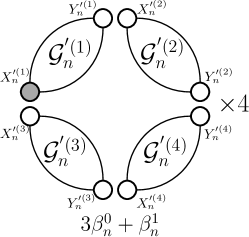
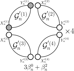
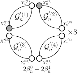
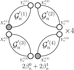
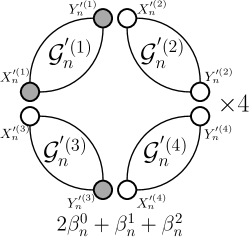
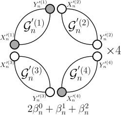
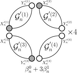
Figure 11: Illustration of all possible configurations and their sizes of matchings for graph $\mathcal{G}^{\prime}_{n+1}$ belonging to $\Omega^{1}_{n+1}$, which contain all matchings in $\Theta^{1}_{n+1}$.

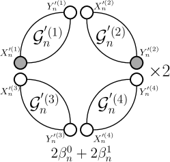
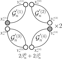
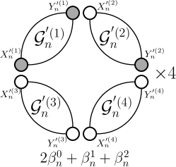
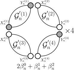
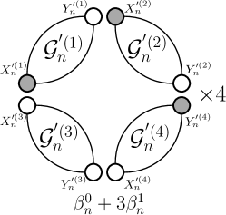
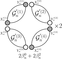
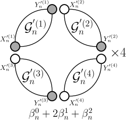
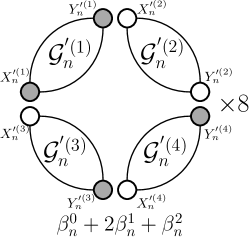
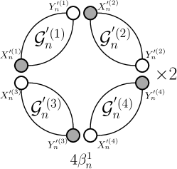
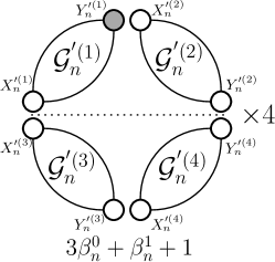
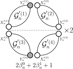
Figure 12: Illustration of all possible configurations and their sizes of matchings for graph $\mathcal{G}^{\prime}_{n+1}$ belonging to $\Omega^{2}_{n+1}$, which contain all matchings in $\Theta^{2}_{n+1}$.

3.2.2 Number of matchings

Let $\theta_{n}$ denote the number of maximum matchings of $\mathcal{G}^{\prime}_{n}$. To calculate $\theta_{n}$, we introduce two additional quantities. Let $\phi_{n}$ be the number of maximum matchings in $\Omega^{0}_{n}$, and let $\varphi_{n}$ be the number of maximum matchings in $\Omega^{1}_{n}$. For small $n$, quantities $\phi_{n}$, $\varphi_{n}$ and $\theta_{n}$ can be easily determined by using a computer. For example, for $n=1$, $\theta_{1}=2$, $\phi_{1}=1$ and $\varphi_{1}=2$. For large $n$, they can be determined recursively as follows.

Theorem 3.7.

For graph $\mathcal{G}_{n}$, $n\geq 1$, the three quantities $\theta_{n}$, $\phi_{n}$ and $\varphi_{n}$ can be calculated recursively according to the following relations:

$$\theta_{n+1}= 2\theta_{n}^{2}\phi_{n}^{2}+2\varphi_{n}^{4}+12\theta_{n}\phi_{n}\varphi_{n}^{2},$$ (9)

$$\phi_{n+1}= 4\phi_{n}^{2}\varphi_{n}^{2},$$ (10)

$$\varphi_{n+1}= 4\theta_{n}\phi_{n}^{2}\varphi_{n}+4\phi_{n}\varphi_{n}^{3}.$$ (11)

with initial conditions $\theta_{1}=2$, $\phi_{1}=1$, and $\varphi_{1}=2$.

Proof 3.8.

We only prove Eq. (10), because the other two equations can be proved analogously. Since for $n\geq 1$, $\beta^{0}_{n}<\beta^{1}_{n}<\beta^{2}_{n}$, according to Eq. (6) and Fig. 10, all maximum matchings with size $\beta^{0}_{n+1}$ in $\Omega^{0}_{n+1}$ are those matchings having size $2\beta^{0}_{n}+2\beta^{1}_{n}$, which together with the symmetry of graph $\mathcal{G}^{\prime}_{n+1}$, yields Eq. (10).

4 Independence number and the number of maximum independence sets

In this section, we study the independence number and the number of MISs in the two studied self-similar scale-free networks.

4.1 Independence number and the number of maximum independence sets in fractal scale-free networks

We first study the independence number and the number of MISs in fractal scale-free graph $\mathcal{G}_{n}$.

4.1.1 Independence number

Let $\alpha_{n}$ denote independence number of graph $\mathcal{G}_{n}$. To find $\alpha_{n}$, we define some intermediate quantities. Note that all the independent sets of $\mathcal{G}_{n}$ can be classified into three types: $\Psi^{0}_{n}$, $\Psi^{1}_{n}$ and $\Psi^{2}_{n}$, where $\Psi^{k}_{n}$, $k=0,1,2$, represent the set of independent sets, each including exactly $k$ initial vertices of $\mathcal{G}_{n}$. Let $\Phi^{k}_{n}$, $k=0,1,2$, be the subset of $\Psi^{k}_{n}$, where each independent set has the largest cardinality, denoted as $\alpha^{k}_{n}$, $k=0,1,2$. Then, $\alpha_{n}$ can be represented as $\alpha_{n}={\rm max}\{\alpha^{0}_{n},\alpha^{1}_{n},\alpha^{2}_{n}\}$.

Theorem 4.1.

The independence number of graph $\mathcal{G}_{n}$, $n\geq 1$, is $\alpha_{n}=2^{2n-2}$.

Proof 4.2.

Since $\alpha_{n}={\rm max}\{\alpha^{0}_{n},\alpha^{1}_{n},\alpha^{2}_{n}\}$, the problem of determining $\alpha_{n}$ is reduced to evaluating the three quantities $\alpha^{0}_{n}$, $\alpha^{1}_{n}$ and $\alpha^{2}_{n}$. By using the self-similar structure, it is not difficult to prove that quantities $\alpha^{0}_{n}$, $\alpha^{1}_{n}$ and $\alpha^{2}_{n}$ satisfy the following relations:

$$\alpha^{0}_{n+1} ={\rm max}\{4\alpha^{0}_{n},2\alpha^{0}_{n}+2\alpha^{1}_{n}-1\}\,,$$ (12)

$$\alpha^{1}_{n+1} ={\rm max}\{2\alpha^{0}_{n}+2\alpha^{1}_{n}-1,\alpha^{0}_{n}+2\alpha^{1}_{n}+\alpha^{2}_{n}-2\}\,,$$ (13)

$$\alpha^{2}_{n+1} ={\rm max}\{2\alpha^{1}_{n}+2\alpha^{2}_{n}-3,4\alpha^{1}_{n}-2\}\,.$$ (14)

By definition, $\alpha_{n+1}^{k}$, $k=0,1,2$, is the cardinality of an independent set in $\Psi^{k}_{n}$. Below, we will show that $\Psi^{0}_{n+1}$, $\Psi^{1}_{n+1}$, and $\Psi^{2}_{n+1}$ can be iteratively constructed from $\Psi^{0}_{n}$, $\Psi^{1}_{n}$, and $\Psi^{2}_{n}$. Thus, $\alpha_{n+1}^{0}$, $\alpha_{n+1}^{1}$, and $\alpha_{n+1}^{0}$ can be expressed in terms of $\alpha_{n}^{0}$, $\alpha_{n}^{1}$, and $\alpha_{n}^{2}$. We now prove graphically the above recursive relations given by Eqs. (12), (13), and (14).

We first prove Eq. (12). By the second construction, $\mathcal{G}_{n+1}$ consists of four copies of $\mathcal{G}_{n}$, $\mathcal{G}_{n}^{(\theta)}$, $\theta=1,2,3,4$. By definition, for any independent set $\chi$ in $\Psi_{n+1}^{0}$, the two initial vertices $X_{n+1}$ and $Y_{n+1}$ of $\mathcal{G}_{n+1}$ do not belong to $\chi$, implying that the corresponding two pairs ($X_{n}^{(1)}$ and $X_{n}^{(3)}$, $Y_{n}^{(2)}$ and $Y_{n}^{(4)}$) of the identified initial vertices of $\mathcal{G}_{n}^{(\theta)}$, $\theta=1,2,3,4$, are not in $\chi$. In addition, since the two hub vertices $W_{n+1}$ and $Z_{n+1}$ of $\mathcal{G}_{n+1}$ are adjacent, at most one of them is in $\chi$, meaning that among the two pairs of vertices ($Y_{n}^{(1)}$ and $X_{n}^{(2)}$, $Y_{n}^{(3)}$ and $X_{n}^{(4)}$), at most one pair is in $\chi$, see Fig. 13. Therefore, we can construct set $\chi$ only from $\Psi_{n}^{0}$ and $\Psi_{n}^{1}$ by considering whether the initial vertices of $\mathcal{G}_{n}^{(\theta)}$, $\theta=1,2,3,4$, are in $\chi$ or not. Figure 13 illustrates all possible configurations of independent sets in $\Phi_{n+1}^{0}$ that include $\Psi_{n+1}^{0}$ as its subset. From Fig. 13, we obtain Eq. (12).

Similarly we can prove Eqs. (13) and (14), the graphical representations of which are shown in Figs. 14 and 15, respectively.

Considering the initial conditions $\alpha^{0}_{1}=1$, $\alpha^{1}_{1}=1$, and $\alpha^{2}_{1}=2$, Eqs. (12), (13), and (14) are solved to yield $\alpha^{0}_{n}=2^{2n-2}$, $\alpha^{1}_{n}=2^{2n-2}-2^{n-1}+1$, and $\alpha^{2}_{n}=2^{2n-2}-(n-1)2^{n-1}+1$. Thus, $\alpha_{n}={\rm max}\{\alpha^{0}_{n},\alpha^{1}_{n},\alpha^{2}_{n}\}=2^{2n-2}$.

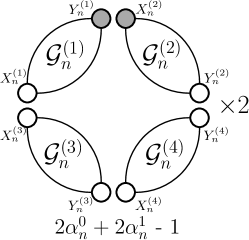
Figure 13: Illustration of all possible configurations and their sizes of independent sets $\Psi^{0}_{n+1}$ in graph $\mathcal{G}_{n+1}$, which contain all independent sets in $\Phi^{0}_{n+1}$.

Figure 14: Illustration of all possible configurations and their sizes of independent sets $\Psi^{1}_{n+1}$ in graph $\mathcal{G}_{n+1}$, which contain all independent sets in $\Phi^{1}_{n+1}$.

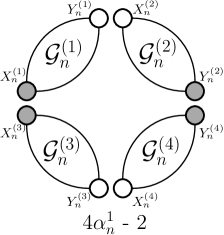
Figure 15: Illustration of all possible configurations and their sizes of independent sets $\Psi^{2}_{n+1}$ in graph $\mathcal{G}_{n+1}$, which contain all independent sets in $\Phi^{2}_{n+1}$.

4.1.2 Number of maximum independent sets

In addition the independence number, the number of MISs in graph $\mathcal{G}_{n}$ can also be determined exactly.

Theorem 4.3.

The number of maximum independent sets in graph $\mathcal{G}_{n}$, $n\geq 1$, is $2^{2^{2n-2}}$.

Proof 4.4.

From the proof of Theorem 4.1, we have $\alpha^{0}_{n}>\alpha^{1}_{n}>\alpha^{2}_{n}$ when $n\geq 2$. Thus, according to Eq. (12), $\alpha^{0}_{n+1}={\rm max}\{4\alpha^{0}_{n},2\alpha^{0}_{n}+2\alpha^{1}_{n}-1\}=4\alpha^{0}_{n}$. Let $x_{n}$ denote the number of MISs in graph $\mathcal{G}_{n}$. From Fig. 13, we obtain

$$x_{n+1}=x_{n}^{4},$$ (15)

which, under the initial value $x_{1}=2$, is solved to yield $x_{n}=2^{2^{2n-2}}$.

Theorem 4.3 shows that number of MISs in graph $\mathcal{G}_{n}$ grows exponentially with the number of vertices $N_{n}$ .

4.2 Independence number and the number of maximum independent sets in non-fractal scale-free networks

We continue to study the independence number and the number of MISs in non-fractal scale-free graph $\mathcal{G}^{\prime}_{n}$.

4.2.1 Independence number

We classify all the independent sets of $\mathcal{G}^{\prime}_{n}$ into two types: $\Psi^{0}_{n}$ and $\Psi^{1}_{n}$, where $\Psi^{k}_{n}$, $k=0,1,2$, represent the set of independent sets, each including exactly $k$ hub vertices of $\mathcal{G}^{\prime}_{n}$. Let $\Phi^{k}_{n}$, $k=0,1,2$, be the subset of $\Psi^{k}_{n}$, where each independent set has the largest cardinality, denoted by $\alpha^{k}_{n}$, $k=0,1,2$. Since there is an edge connecting the two hub vertices $X^{\prime}_{n}$ and $Y^{\prime}_{n}$, set $\Psi^{2}_{n}$ is empty, implying $\alpha^{2}_{n}=0$. Let $\alpha_{n}$ denote the independence number of $\mathcal{G}^{\prime}_{n}$. Then, $\alpha_{n}$ can be expressed as $\alpha_{n}={\rm max}\{\alpha^{0}_{n},\alpha^{1}_{n}\}$.

Theorem 4.5.

The independence number of graph $\mathcal{G}^{\prime}_{n}$, $n\geq 1$, is $\alpha_{n}=2^{2n-1}$.

Proof 4.6.

Considering $\alpha_{n}={\rm max}\{\alpha^{0}_{n},\alpha^{1}_{n}\}$, in order to determine, we alternatively evaluate the two quantities $\alpha^{0}_{n}$ and $\alpha^{1}_{n}$ by using the self-similarity of the graph. First, we show that $\alpha^{0}_{n}$ and $\alpha^{1}_{n}$ obey the following recursion relations:

$$\alpha^{0}_{n+1} ={\rm max}\{4\alpha^{0}_{n},2\alpha^{0}_{n}+2\alpha^{1}_{n}-1,4\alpha^{1}_{n}-2\}\,,$$ (16)

$$\alpha^{1}_{n+1} =2\alpha^{0}_{n}+2\alpha^{1}_{n}-1\,.$$ (17)

Equations (16) and (17) be proved graphically. Figures 16, and 17 show the graphical representations of Eqs. (16) and (17), respectively.

Using the initial conditions $\alpha^{0}_{1}=2$ and $\alpha^{1}_{1}=1$, Eqs. (16) and (17) are solved to yield exact solutions for $\alpha^{0}_{n}$ and $\alpha^{1}_{n}$ as $\alpha^{0}_{n}=2^{2n-1}$ and $\alpha^{1}_{n}=2^{2n-1}-2^{n}+1$. Then, we have $\alpha_{n}={\rm max}\{\alpha^{0}_{n},\alpha^{1}_{n}\}=2^{2n-1}$ for $n\geq 1$.

Figure 16: Illustration of all possible configurations and their sizes of independent sets $\Psi^{0}_{n+1}$ in graph $\mathcal{G}^{\prime}_{n+1}$, which contain all independent sets in $\Phi^{0}_{n+1}$.

Figure 17: Illustration of all possible configurations and their sizes of independent sets $\Psi^{1}_{n+1}$ in graph $\mathcal{G}^{\prime}_{n+1}$, which contain all independent sets in $\Phi^{1}_{n+1}$.

4.2.2 Number of maximum independence sets

In contrast to the its fractal counterpart $\mathcal{G}_{n}$, the non-fractal scale-free graph $\mathcal{G^{\prime}}_{n}$ has only one maximum independence set for all $n\geq 1$.

Theorem 4.7.

In the non-fractal scale-free graph $\mathcal{G^{\prime}}_{n}$, $n\geq 1$, there exists a unique maximum independence set.

Proof 4.8.

Let $x_{n}$ denote the number of MISs in $\mathcal{G}^{\prime}_{n}$. Equation (16) and Fig. 16 show that for $n\geq 2$ any MIS of $\mathcal{G}^{\prime}_{n+1}$ is in fact the union of maximum independent sets in $\Phi_{n}^{0}$, of the four copies of $\mathcal{G}^{\prime}_{n}$ (i.e. $\mathcal{G}_{n}^{{}^{\prime}(1)}$, $\mathcal{G}_{n}^{{}^{\prime}(2)}$, $\mathcal{G}_{n}^{{}^{\prime}(3)}$, and $\mathcal{G}_{n}^{{}^{\prime}(4)}$) forming $\mathcal{G}^{\prime}_{n+1}$. Thus, any MIS of $\mathcal{G}_{n+1}$ is determined by those of $\mathcal{G}_{n}^{{}^{\prime}(1)}$, $\mathcal{G}_{n}^{{}^{\prime}(2)}$, $\mathcal{G}_{n}^{{}^{\prime}(3)}$, and $\mathcal{G}_{n}^{{}^{\prime}(4)}$. Moreover, $x_{n+1}=x_{n}^{4}$. Since $x_{1}=1$, we have $x_{n}=1$ for all $n\geq 1$.

Theorem 4.7 indicates that for all $n\geq 1$, $\mathcal{G}^{\prime}_{n}$ is a unique independence graph. Furthermore, it is easy to see that the unique MIS of $\mathcal{G}^{\prime}_{n}$, $n\geq 1$, contains exactly all the vertices with degree two that are generated at iteration $n-1$.

5 Domination number and the number of minimum dominating sets

In this section, we study the domination number and the number of MDSs in two self-similar scale-free networks $\mathcal{G}_{n}$ and $\mathcal{G}^{\prime}_{n}$.

5.1 Domination number and the number of MDSs in fractal scale-free networks

We first study the domination number and the number of MDSs in the fractal scale-free network $\mathcal{G}_{n}$.

Let $\gamma_{n}$ denote the domination number of graph $\mathcal{G}_{n}$. In order to determine $\gamma_{n}$, we classify into all the dominating sets of $\mathcal{G}_{n}$ into three groups: $\Gamma^{0}_{n}$, $\Gamma^{1}_{n}$ and $\Gamma^{2}_{n}$, where $\Gamma^{k}_{n}$, $k=0,1,2$, represent the set of those dominating sets including exactly $k$ initial vertices of $\mathcal{G}_{n}$. Moreover, let $\Upsilon^{k}_{n}$, $k=0,1,2$, be the subset of $\Upsilon^{k}_{n}$, where each independent set has the largest cardinality, denoted as $\gamma^{k}_{n}$, $k=0,1,2$. By definition, we have $\gamma_{n}={\rm min}\{\gamma^{0}_{n},\gamma^{1}_{n},\gamma^{2}_{n}\}$.

Theorem 5.1.

For $n\geq 2$, the domination number of graph $\mathcal{G}_{n}$ is $\gamma_{n}=\frac{5\cdot 2^{2n-4}+4}{3}$.

Proof 5.2.

Since the problem of determining $\gamma_{n}$ can be reduced to finding $\gamma^{0}_{n}$, $\gamma^{1}_{n}$ and $\gamma^{2}_{n}$, we now determine these three intermediate quantities. To this end, we provide the following recursion relation for $n\geq 2$ governing these quantities:

$$\gamma^{0}_{n+1} ={\rm min}\{4\gamma^{0}_{n},2\gamma^{0}_{n}+2\gamma^{1}_{n}-1,4\gamma^{1}_{n}-2\}\,,$$ (18)

$$\gamma^{1}_{n+1} ={\rm min}\{2\gamma^{0}_{n}+2\gamma^{1}_{n}-1,\gamma^{0}_{n}+2\gamma^{1}_{n}+\gamma^{1}_{n}-2,$$

$$\quad\quad\quad\quad 2\gamma^{1}_{n}+2\gamma^{2}_{n}-3\}\,,$$ (19)

$$\gamma^{2}_{n+1} ={\rm min}\{4\gamma^{1}_{n}-2,2\gamma^{1}_{n}+2\gamma^{2}_{n}-3,4\gamma^{2}_{n}-4\}\,.$$ (20)

Equations (18), (19), and (20) can all be proved graphically.

We first prove Eq. (18). According to Fig. 3, $\mathcal{G}_{n+1}$ is consist of four copies of $\mathcal{G}_{n}$, $\mathcal{G}_{n}^{(\theta)}$, $\theta=1,2,3,4$. By definition, for any dominating set $\xi$ in $\Upsilon_{n+1}^{0}$, both of the two initial vertices $X_{n+1}$ and $Y_{n+1}$ of $\mathcal{G}_{n+1}$ are not in $\xi$, implying that the corresponding two pairs ($X_{n}^{(1)}$ and $X_{n}^{(3)}$, $Y_{n}^{(2)}$ and $Y_{n}^{(4)}$) of identified initial vertices of $\mathcal{G}_{n}^{(\theta)}$, $\theta=1,2,3,4$, are not in $\xi$. In addition, according to the number of hub vertices in a dominating sets belonging $\Upsilon_{n+1}^{0}$, the dominating sets in $\Upsilon_{n+1}^{0}$ can be further sorted into three disjoint subsets. Figure 18 illustrates all possible configurations of dominating sets in $\Gamma_{n+1}^{0}$ that contains all dominating sets in $\Upsilon_{n+1}^{0}$. In Fig. 18, only the initial vertices of $\mathcal{G}_{n}^{(\theta)}$, $\theta=1,2,3,4$, are shown, with solid vertices being in the dominating sets, while open vertices not. From Fig. 18, we establish Eq. (18).

In a similar way, we can prove Eqs. (19) and (20), the graphical representations of which are provided in Figs. 19 and 20, respectively.

With initial condition $\gamma^{0}_{2}=4$, $\gamma^{1}_{2}=3$ and $\gamma^{2}_{2}=3$, Eqs. (18), (19), and (20) are solved to yield $\gamma^{0}_{n}=\frac{5\cdot 2^{2n-4}+3\cdot 2^{n-1}-2}{3}$, $\gamma^{1}_{n}=\frac{5\cdot 2^{2n-4}+3\cdot 2^{n-2}+1}{3}$, and $\gamma^{2}_{n}=\frac{5\cdot 2^{2n-4}+4}{3}$. Thus, the domination number of graph $\mathcal{G}_{n}$ is $\gamma_{n}={\rm min}\{\gamma^{0}_{n},\gamma^{1}_{n},\gamma^{2}_{n}\}=\gamma^{2}_{n}=\frac{5\cdot 2^{2n-4}+4}{3}$ for all $n\geq 2$.

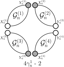
Figure 18: Illustration of all possible configurations and their sizes of dominating sets $\Gamma^{0}_{n+1}$ in graph $\mathcal{G}_{n+1}$ containing $\Upsilon^{0}_{n+1}$.

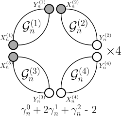
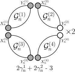
Figure 19: Illustration of all possible configurations and their sizes of dominating sets $\Gamma^{1}_{n+1}$ in graph $\mathcal{G}_{n+1}$ containing $\Upsilon^{1}_{n+1}$.

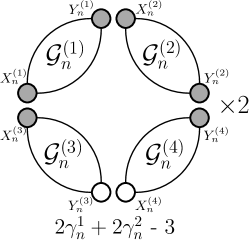
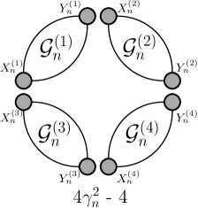
Figure 20: Illustration of all possible configurations and their sizes of dominating sets $\Gamma^{2}_{n+1}$ in graph $\mathcal{G}_{n+1}$ containing $\Upsilon^{2}_{n+1}$.

5.1.1 Number of minimum dominating sets

In addition the domination number, the number of MDSs in graph $\mathcal{G}_{n}$ can also be determined exactly.

Theorem 5.3.

The number of maximum dominating sets in graph $\mathcal{G}_{n}$, $n\geq 2$, is $2^{2^{2n-4}}$.

Proof 5.4.

Let $y_{n}$ denote the number of MDSs in graph $\mathcal{G}_{n}$. From Eq. (20) and Fig. 13, we know that for $n\geq 2$, any MDS of $\mathcal{G}_{n+1}$ is in fact the union of MDSs in $\Upsilon_{n}^{2}$, of the four copies of $\mathcal{G}_{n}$ (i.e. $\mathcal{G}_{n}^{(1)}$, $\mathcal{G}_{n}^{(2)}$, $\mathcal{G}_{n}^{(3)}$, and $\mathcal{G}_{n}^{(4)}$) constituting $\mathcal{G}_{n+1}$. Therefore, we obtain

$$y_{n+1}=y_{n}^{4},$$ (21)

which, under the initial value $y_{2}=2$, is solved to yield $x_{n}=2^{2^{2n-4}}$.

Theorem 5.3 shows that the number of MDSs in graph $\mathcal{G}_{n}$ grows exponentially with the number of vertices $N_{n}$, which is similar to the number of MISs.

5.2 Domination number and the number of minimum dominating sets in non-fractal scale-free networks

We finally study the domination number and the number of MDSs in the non-fractal scale-free network $\mathcal{G}^{\prime}_{n}$.

Analogously to graph $\mathcal{G}^{\prime}_{n}$, all the dominating sets in $\mathcal{G}^{\prime}_{n}$ can be classified into three sets: $\Gamma^{0}_{n}$, $\Gamma^{1}_{n}$ and $\Gamma^{2}_{n}$, where $\Gamma^{k}_{n}$, $k=0,1,2$, represent the set of dominating sets, each including exactly $k$ hub vertices of $\mathcal{G}^{\prime}_{n}$. Let $\Upsilon^{k}_{n}$, $k=0,1,2$, be the subset of $\Gamma^{k}_{n}$, where each independent set has the smallest cardinality, denoted by $\gamma^{k}_{n}$, $k=0,1,2$. Then, the domination number $\gamma_{n}$ of $\mathcal{G}^{\prime}_{n}$ can be expressed by $\gamma_{n}={\rm min}\{\gamma^{0}_{n},\gamma^{1}_{n},\gamma^{2}_{n}\}$.

Theorem 5.5.

For $n\geq 3$, the domination number of non-fractal scale-free graph $\mathcal{G}^{\prime}_{n}$ is $\gamma_{n}=\frac{2^{2n-3}+4}{3}$.

Proof 5.6.

Since $\gamma_{n}={\rm min}\{\gamma^{0}_{n},\gamma^{1}_{n},\gamma^{2}_{n}\}$, we first evaluate the quantities $\gamma^{0}_{n}$, $\gamma^{1}_{n}$ and $\gamma^{2}_{n}$. In a way similar to the case of graph $\mathcal{G}_{n}$, we establish the following recursive relations governing the three quantities $\gamma^{0}_{n}$, $\gamma^{1}_{n}$ and $\gamma^{2}_{n}$:

$$\gamma^{0}_{n+1} ={\rm min}\{4\gamma^{0}_{n},2\gamma^{0}_{n}+2\gamma^{1}_{n}-1,4\gamma^{1}_{n}-2\}\,,$$ (22)

$$\gamma^{1}_{n+1} ={\rm min}\{2\gamma^{0}_{n}+2\gamma^{1}_{n}-1,\gamma^{0}_{n}+2\gamma^{1}_{n}+\gamma^{1}_{n}-2,$$

$$\quad\quad\quad\quad 2\gamma^{1}_{n}+2\gamma^{2}_{n}-3\}\,,$$ (23)

$$\gamma^{2}_{n+1} ={\rm min}\{4\gamma^{1}_{n}-2,2\gamma^{1}_{n}+2\gamma^{2}_{n}-3,4\gamma^{2}_{n}-4\}\,.$$ (24)

Figures 21, 22, and 23 show, respectively, all the possible configurations of dominating sets $\Gamma^{0}_{n+1}$, $\Gamma^{1}_{n+1}$, and $\Gamma^{2}_{n+1}$ for graph $\mathcal{G}^{\prime}_{n+1}$. From these three figures, we can establish Eqs. (22), (23), and (24). By using the initial conditions $\gamma^{0}_{3}=8$, $\gamma^{1}_{3}=7$ and $\gamma^{2}_{3}=4$, Eqs. (22), (23), and (24) are solved to yield $\gamma^{0}_{n}=\frac{2^{2n-3}+3\cdot 2^{n}-2}{3}$, $\gamma^{1}_{n}=\frac{2^{2n-3}+3\cdot 2^{n-1}+1}{3}$ and $\gamma^{2}_{n}=\frac{2^{2n-3}+4}{3}$. Hence, $\gamma_{n}={\rm min}\{\gamma^{0}_{n},\gamma^{1}_{n},\gamma^{2}_{n}\}=\gamma^{2}_{n}=\frac{2^{2n-3}+4}{3}$.

Figure 21: Illustration of all possible configurations and their sizes of dominating sets $\Gamma^{0}_{n+1}$ in graph $\mathcal{G}^{\prime}_{n+1}$ containing $\Upsilon^{0}_{n+1}$.

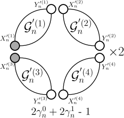
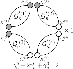
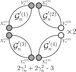
Figure 22: Illustration of all possible configurations and their sizes of dominating sets $\Gamma^{1}_{n+1}$ in graph $\mathcal{G}^{\prime}_{n+1}$ containing $\Upsilon^{1}_{n+1}$.

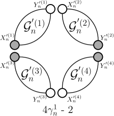
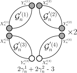
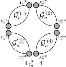
Figure 23: Illustration of all possible configurations and their sizes of dominating sets $\Gamma^{2}_{n+1}$ in graph $\mathcal{G}^{\prime}_{n+1}$ containing $\Upsilon^{2}_{n+1}$.

5.2.1 Number of minimum dominating sets

In contrast to the its fractal counterpart $\mathcal{G}_{n}$, the non-fractal scale-free graph $\mathcal{G}^{\prime}_{n}$ has only one maximum independence set for all $n\geq 3$.

Theorem 5.7.

In the non-fractal scale-free graph $\mathcal{G}^{\prime}_{n}$, $n\geq 3$, there exists a unique minimum dominating set.

Proof 5.8.

Denote by $y_{n}$ the number of MDSs in $\mathcal{G}^{\prime}_{n}$. Eq. (24) and Fig. 23 show that for $n\geq 3$, any MDS of $\mathcal{G}^{\prime}_{n+1}$ is actually the union of MDSs in $\Upsilon_{n}^{2}$, of the four copies of $\mathcal{G}^{\prime}_{n}$ (i.e. $\mathcal{G}_{n}^{{}^{\prime}(1)}$, $\mathcal{G}_{n}^{{}^{\prime}(2)}$, $\mathcal{G}_{n}^{{}^{\prime}(3)}$, and $\mathcal{G}_{n}^{{}^{\prime}(4)}$) forming $\mathcal{G}^{\prime}_{n+1}$. Thus, one obtains $y_{n+1}=y_{n}^{4}$, which with the initial value $y_{2}=1$ is solved to give $y_{n}=1$ for all $n\geq 3$.

Theorem 5.7 implies that for all $n\geq 3$, $\mathcal{G}^{\prime}_{n}$ has a unique MDS. Moreover, the unique MDSs of $\mathcal{G}^{\prime}_{n}$, $n\geq 3$, in fact contains exactly all the hub and border vertices in graph $\mathcal{G}^{\prime}_{n-1}$.

6 Conclusion

Many real-world networks simultaneously display the striking scale-free and self-similar properties. Prior works have shown that the scale-free topology has an substantial effects on the various properties of graphs, e.g., combinatorial properties. In this paper, we studied some combinatorial problems for two self-similar scale-free networks with identical power exponent, both of which are constructed in an iterative manner. At any iteration, the two networks have the same number of vertices and the same number of edges. Although both networks bear some resemblance, they differ in some aspects. For example, the first one is “large-world” and fractal, while the second one is small-world and non-fractal. By using their self-similarity and decimation technique, we provide exact expressions for the maximum number, the matching number, the independence number, and the domination number for both networks. Moreover, we find exact or recursive solutions to the number of maximum matchings, the number of MISs, and the number of MDSs for both graphs.

For the maximum matching problem, the matching number of the fractal graph is about twice that of the non-fractal graph, but in both graphs the number of maximum matchings grows exponentially with the number of total edges in the graphs. With respect to the MIS problem, the independence number of the first network is exactly half of the second network. In addition, the number of the MISs in the first graph grows exponentially with the number of vertices in the graph. In contrast, the second graph has a unique MIS. Finally, as for the MDS problem, the domination number of the fractal graph is about twice as large as its non-fractal counterpart. Moreover, the number of the MDSs in the fractal graph grows exponentially with the vertex number, while there exists a unique MDS in the non-fractal graph. Thus, although both graphs are self-similar and scale-free with the same vertex number, edge number, and power exponent, they greatly differ in the studied combinatorial aspects. Our results show that scale-free topology itself is not sufficient to characterize combinatorial properties in power-law graphs. Given the relevance of combinatorial problems to various practical scenarios, our work sheds light on better understanding the applications of combinatorial properties for scale-free networks.

Data Availability Statement

No new data were generated or analysed in support of this research.

References

- [1] Hopkins, G. and Staton, W. (1985) Graphs with unique maximum independent sets. Discrete Math., 57, 245–251.
- [2] Montroll, E. W. (1964) Lattice statistics. In Beckenbach, E. (ed.), Applied Combinatorial Mathematics, pp. 96–143. Wiley, New York.
- [3] Vukičević, D. (2011) Applications of perfect matchings in chemistry. In Dehmer, M. (ed.), Structural Analysis of Complex Networks, pp. 463–482. Birkhäuser Boston.
- [4] Lovász, L. and Plummer, M. D. (1986) Matching Theory, Annals of Discrete Mathematics, 29. North Holland, New York.
- [5] Karp, R. M. (1972) Reducibility among combinatorial problems. Complexity of Computer Computations, pp. 85–103. Springer.
- [6] Pardalos, P. M. and Xue, J. (1994) The maximum clique problem. J. Global Optim., 4, 301–328.
- [7] Araujo, F., Farinha, J., Domingues, P., Silaghi, G. C., and Kondo, D. (2011) A maximum independent set approach for collusion detection in voting pools. J. Parallel Distrib. Comput., 71, 1356–1366.
- [8] Joo, C., Lin, X., Ryu, J., and Shroff, N. B. (2016) Distributed greedy approximation to maximum weighted independent set for scheduling with fading channels. IEEE/ACM Trans. Netw., 24, 1476–1488.
- [9] Shen, C. and Li, T. Multi-document summarization via the minimum dominating set. Proceedings of the 23rd International Conference on Computational Linguistics, 2010, pp. 984–992. Association for Computational Linguistics.
- [10] Wu, J. (2002) Extended dominating-set-based routing in ad hoc wireless networks with unidirectional links. IEEE Trans. Parallel Distrib. Syst., 13, 866–881.
- [11] Wuchty, S. (2014) Controllability in protein interaction networks. Proc. Natl. Acad. Sci. USA, 111, 7156–7160.
- [12] Liu, Y. Y. and Barabási, A.-L. (2016) Control principles of complex systems. Rev. Mod. Phys., 88, 035006.
- [13] Liu, Y.-Y., Slotine, J.-J., and Barabási, A.-L. (2011) Controllability of complex networks. Nature, 473, 167–173.
- [14] Nepusz, T. and Vicsek, T. (2012) Controlling edge dynamics in complex networks. Nature Phys., 8, 568–573.
- [15] Yan, W. and Zhang, F. (2005) Graphical condensation for enumerating perfect matchings. J. Comb. Theory Ser. A, 110, 113 – 125.
- [16] Yan, W. and Zhang, F. (2008) A quadratic identity for the number of perfect matchings of plane graphs. Theor. Comput. Sci., 409, 405–410.
- [17] Chebolu, P., Frieze, A., and Melsted, P. (2010) Finding a maximum matching in a sparse random graph in expected time. J. ACM, 57, 24.
- [18] Yuster, R. (2013) Maximum matching in regular and almost regular graphs. Algorithmica, 66, 87–92.
- [19] Zhang, Z. and Wu, B. (2015) Pfaffian orientations and perfect matchings of scale-free networks. Theoret. Comput. Sci., 570, 55–69.
- [20] Li, H. and Zhang, Z. (2017) Maximum matchings in scale-free networks with identical degree distribution. Theoret. Comput. Sci., 675, 64–81.
- [21] Xiao, M. and Nagamochi, H. (2013) Confining sets and avoiding bottleneck cases: A simple maximum independent set algorithm in degree-3 graphs. Theoret. Comput. Sci., 469, 92–104.
- [22] Hon, W.-K., Kloks, T., Liu, C.-H., Liu, H.-H., Poon, S.-H., and Wang, Y.-L. (2015) On maximum independent set of categorical product and ultimate categorical ratios of graphs. Theoret. Comput. Sci., 588, 81–95.
- [23] Chuzhoy, J. and Ene, A. (2016) On approximating maximum independent set of rectangles. Proceedings of IEEE 2016 Annual Symposium on Foundations of Computer Science, pp. 820–829. IEEE.
- [24] Fomin, F. V., Grandoni, F., Pyatkin, A. V., and Stepanov, A. A. (2008) Combinatorial bounds via measure and conquer: Bounding minimal dominating sets and applications. ACM Tran. Algorithms, 5, 9.
- [25] Hedar, A.-R. and Ismail, R. (2012) Simulated annealing with stochastic local search for minimum dominating set problem. Int. J. Mach. Learn. Cybernet., 3, 97–109.
- [26] Nacher, J. C. and Akutsu, T. (2012) Dominating scale-free networks with variable scaling exponent: heterogeneous networks are not difficult to control. New J. Phys., 14, 073005.
- [27] Gast, M., Hauptmann, M., and Karpinski, M. (2015) Inapproximability of dominating set on power law graphs. Theoret. Comput. Sci., 562, 436–452.
- [28] Shan, L., Li, H., and Zhang, Z. (2017) Domination number and minimum dominating sets in pseudofractal scale-free web and Sierpiński graph. Theoret. Comput. Sci., 677, 12–30.
- [29] Haynes, T. W., Hedetniemi, S., and Slater, P. (1998) Fundamentals of Domination in Graphs. Marcel Dekker, New York.
- [30] Robson, J. M. (1986) Algorithms for maximum independent sets. J. Algorithms, 7, 425–440.
- [31] Halldórsson, M. M. and Radhakrishnan, J. (1997) Greed is good: Approximating independent sets in sparse and bounded-degree graphs. Algorithmica, 18, 145–163.
- [32] Valiant, L. (1979) The complexity of computing the permanent. Theor. Comput. Sci., 8, 189–201.
- [33] Valiant, L. (1979) The complexity of enumeration and reliability problems. SIAM J. Comput., 8, 410–421.
- [34] Newman, M. E. J. (2003) The structure and function of complex networks. SIAM Rev., 45, 167–256.
- [35] Barabási, A. and Albert, R. (1999) Emergence of scaling in random networks. Science, 286, 509–512.
- [36] Chung, F. and Lu, L. (2002) The average distances in random graphs with given expected degrees. Proc. Natl. Acad. Sci., 99, 15879–15882.
- [37] Albert, R., Jeong, H., and Barabási, A.-L. (2000) Error and attack tolerance of complex networks. Nature, 406, 378.
- [38] Chakrabarti, D., Wang, Y., Wang, C., Leskovec, J., and Faloutsos, C. (2008) Epidemic thresholds in real networks. ACM Trans. Inform. Syst. Secur., 10, 13.
- [39] Yi, Y., Zhang, Z., and Patterson, S. (2020) Scale-free loopy structure is resistant to noise in consensus dynamics in complex networks. IEEE Trans. Cybern., 50, 190–200.
- [40] Shan, L., Li, H., and Zhang, Z. (2018) Independence number and the number of maximum independent sets in pseudofractal scale-free web and Sierpiński gasket. Theoret. Comput. Sci., 720, 47–54.
- [41] Ferrante, A., Pandurangan, G., and Park, K. (2008) On the hardness of optimization in power-law graphs. Theoret. Comput. Sci., 393, 220–230.
- [42] Song, C., Havlin, S., and Makse, H. (2005) Self-similarity of complex networks. Nature, 433, 392–395.
- [43] Zhang, Z., Liu, H., Wu, B., and Zou, T. (2011) Spanning trees in a fractal scale-free lattice. Phys. Rev. E, 83, 016116.
- [44] Hinczewski, M. and Berker, A. N. (2006) Inverted Berezinskii-Kosterlitz-Thouless singularity and high-temperature algebraic order in an Ising model on a scale-free hierarchical-lattice small-world network. Phys. Rev. E, 73, 066126.