Serial interconnections of $1$-contracting and $2$-contracting systems

Abstract

The flow of contracting systems contracts 1-dimensional polygons (i.e. lines) at an exponential rate. One reason for the usefulness of contracting systems is that many interconnections of contracting sub-systems yield an overall contracting system. A recent generalization of contracting systems is called $k$-contracting systems, where $k\in\{1,\dots,n\}$. The flow of such systems contracts $k$-dimensional polygons at an exponential rate, and in particular they reduce to contracting systems when $k=1$. Here, we analyze serial interconnections of $1$-contracting and $2$-contracting systems. We provide conditions guaranteeing that such interconnections have a well-ordered asymptotic behaviour, and demonstrate the theoretical results using several examples.

I Introduction

Contracting systems have found numerous applications in systems and control theory. This is due to several reasons. First, contracting systems have a well-ordered behaviour: any two trajectories approach one another at an exponential rate [1]. In particular, if an equilibrium point exists then it is unique and globally exponentially stable. If the vector field is $T$-periodic then the system entrains, i.e. all solutions converge exponentially to a unique $T$-periodic trajectory [1, 2]. In fact, contracting systems have a well-defined frequency response, as shown in [3] in the context of convergent systems [4]. Second, there exist simple sufficient conditions for contraction based on matrix measures [1, 5]. Third, various interconnections of contracting systems, including parallel, serial, and feedback connections, yield an overall contracting system [1, 6].

Ref. [7] studied a generalization called $k$-contraction (see also the note [8]), with $k\in\{1,\dots,n\}$. The flow of such systems contracts $k$-dimensional polygons at an exponential rate. In particular, for $k=1$ these are just standard contracting systems. This generalization is motivated in part by the seminal work by Muldowney and his colleagues [9, 10], on systems that, using the new terminology, are $2$-contracting in a constant metric. Roughly speaking, every bounded solution of a time-invariant $2$-contracting system converges to an equilibrium point. This is different from the case of $1$-contracting systems, as the equilibrium point is not necessarily unique.

Contraction theory is an active area of research. Recent contributions include contraction on Riemannian manifolds [11], various notions of “weak contraction” (see, e.g. [12, 13]), contraction of piecewise-smooth dynamical systems [14], analysis of learning algorithms using contraction theory [15], and the introduction of $\alpha$-contracting systems, with $\alpha\geq 1$ real, which is motivated in part by the seminal works of Douady and Oesterlé [16], and Leonov and his colleagues (see the recent monograph by Kuznetsov and Reitmann [17]) on bounding the Hausdorff dimension of complex attractors.

Since many interconnections of contracting systems yield an overall contracting system, it is natural to ask if the same holds for $k$-contracting systems as well [8]. Here, we address this question in some detail for $k$-contracting systems with $k\in\{1,2\}$. This problem is more delicate than in the case of $1$-contracting systems because the well-ordered behaviour of $2$-contracting systems only holds in the time-invariant case, while connecting two systems implies that at least one system has an input from the other system and thus is time-varying.

Our main contribution is a proof that various serial connections of $k$-contracting systems, with $k\in\{1,2\}$, have a “well-ordered” asymptotic behaviour: they have no non-trivial periodic solutions, and, under stronger assumptions, all solutions converge to an equilibrium point (which is not necessarily unique). We also show that such connections are in general neither $1$-contracting nor $2$-contracting, and thus our results may be used to analyze systems that cannot be studied using only the theory of $2$-contracting systems. To apply our results to wider set of systems, we also provide sufficient conditions guaranteeing that a given system can be decomposed as the serial connection of two systems.

The next section reviews known definitions and results that are used later on. Section III includes the main results, and the final section concludes. Due to space limitations, we focus on theoretical results and provide only a few applications in Section IV. More applications will appear in an extended version of this note that is now in preparation.

We use standard notation. Small [capital] letters denote column vectors [matrices]. $I_{n}$ is the $n\times n$ identity matrix. For a matrix $A$, $A^{T}$ is the transpose of $A$. If $A$ is square, then $|A|$ [$\operatorname{trace}(A)$] is the determinant [trace] of $A$.

II Preliminaries

The sufficient condition for $k$-contraction in [7] is based on the $k$th additive compound of the Jacobian of the vector field. To make this note more accessible, we briefly review these topics. For more details, see also [9]. For more recent applications of these compounds in systems and control theory, see [18, 19, 20, 21, 22].

Let $C\in\mathbb{R}^{n\times m}$. For $k\in\{1,\dots,\min\{n,m\}\}$, the $k$th multiplicative compound of $C$, denoted $C^{(k)}$, is the $\binom{n}{k}\times\binom{m}{k}$ matrix that contains all the $k\times k$ minors of $C$ in lexicographic order [9]. For example, for $n=m=3$ and $k=2$, $C^{(2)}$ is the $3\times 3$ matrix:

$$\begin{bmatrix}\begin{vmatrix}c_{11}&c_{12}\\ c_{21}&c_{22}\end{vmatrix}&\begin{vmatrix}c_{11}&c_{13}\\ c_{21}&c_{23}\end{vmatrix}&\begin{vmatrix}c_{12}&c_{13}\\ c_{22}&c_{23}\end{vmatrix}\\ \begin{vmatrix}c_{11}&c_{12}\\ c_{31}&c_{32}\end{vmatrix}&\begin{vmatrix}c_{11}&c_{13}\\ c_{31}&c_{33}\end{vmatrix}&\begin{vmatrix}c_{12}&c_{13}\\ c_{32}&c_{33}\end{vmatrix}\\ \begin{vmatrix}c_{21}&c_{22}\\ c_{31}&c_{32}\end{vmatrix}&\begin{vmatrix}c_{21}&c_{23}\\ c_{31}&c_{33}\end{vmatrix}&\begin{vmatrix}c_{22}&c_{23}\\ c_{32}&c_{33}\end{vmatrix}\end{bmatrix},$$

where $|B|$ denotes the determinant of $B$. In particular, $C^{(1)}=C$ and if $n=m$ then $C^{(n)}=|C|$. The Cauchy–Binet formula [23, Chapter 0], asserts that for any $B\in\mathbb{R}^{n\times m},C\in\mathbb{R}^{m\times p}$ and any $k\in\{1,\dots,\min\{n,m,p\}\}$, we have

$$(BC)^{(k)}=B^{(k)}C^{(k)}.$$ (1)

This justifies the term multiplicative compound. In particular, (1) implies that if $n=m=p$ then $|BC|=|B||C|$, and that if $A\in\mathbb{R}^{n\times n}$ is non-singular then $(A^{(k)})^{-1}=(A^{-1})^{(k)}$.

Let $A\in\mathbb{R}^{n\times n}$ with eigenvalues $\lambda_{i}$, $i\in\{1,\dots,n\}$. The eigenvalues of $A^{(k)}$ are $\lambda_{i_{1}}\lambda_{i_{2}}\dots\lambda_{i_{k}},$ with $1\leq i_{1}<i_{2}<\dots<i_{k}\leq n$.

For $k\in\{1,\dots,n\}$, the $k$th additive compound of $A$ is the $\binom{n}{k}\times\binom{n}{k}$ matrix defined by

$$A^{[k]}:=\frac{d}{d\varepsilon}(I+\varepsilon A)^{(k)}|_{\varepsilon=0}.$$

In other words, $(I+\varepsilon A)^{(k)}=I+\varepsilon A^{[k]}+o(\varepsilon)$. In particular, $A^{[1]}=A$, and $A^{[n]}=\operatorname{trace}(A).$ The eigenvalues of $A^{[k]}$ are $\lambda_{i_{1}}+\lambda_{i_{2}}+\dots+\lambda_{i_{k}},$ with $1\leq i_{1}<i_{2}<\dots<i_{k}\leq n$.

It is useful to know how these compounds are affected by a coordinate transformation. Let $V\in\mathbb{R}^{m\times n},W\in\mathbb{R}^{n\times p}$. Then (1) yields

$$(VAW)^{(k)}=V^{(k)}A^{(k)}W^{(k)}.$$

If, in addition, $m=p$ and $VW=I_{m}$ then

$$(VAW)^{[k]} =\frac{d}{d\varepsilon}\left(I_{m}+\varepsilon VAW\right)^{(k)}|_{\varepsilon=0}$$

$$=\frac{d}{d\varepsilon}(V(I_{n}+\varepsilon A)W)^{(k)}|_{\varepsilon=0}$$

$$=V^{(k)}A^{[k]}W^{(k)}.$$ (2)

In the context of dynamical systems, the importance of these compounds is due to following fact. If $\Phi:\mathbb{R}_{+}\to\mathbb{R}^{n\times n}$ is the solution of the matrix differential equation

$$\frac{d}{dt}\Phi(t)=A(t)\Phi(t),\quad\Phi(0)=I,$$

where $t\to A(t)$ is continuous, then

$$\frac{d}{dt}(\Phi(t))^{(k)}=(A(t))^{[k]}(\Phi(t))^{(k)}.$$ (3)

In other words, $(\Phi(t))^{(k)}$ also evolves according to a linear dynamics with the matrix $(A(t))^{[k]}$. Roughly speaking, $\Phi^{(k)}$ determines the evolution of $k$-dimensional polygons under the dynamics $\dot{x}=Ax$ [24].

Recall that a vector norm $|\cdot|:\mathbb{R}^{n}\to\mathbb{R}_{+}$ induces a matrix norm $||A||:=\max_{|x|=1}|Ax|$, and a matrix measure $\mu(A):=\lim_{\varepsilon\to 0^{+}}(||I+\varepsilon A||-1)/\varepsilon$. If $\mu((A(t))^{[k]})\leq-\eta<0$ all $t\geq 0$ then applying Coppel’s inequality [25] to (3) yields $||(\Phi(t))^{(k)}||\leq\exp(-\eta t)||(\Phi(0))^{(k)}||$ for all $t\geq 0$. This leads to the following.

Definition 1.

[7] Consider the nonlinear system $\dot{x}(t)=f(t,x(t))$, with $f$ a $C^{1}$ mapping, and suppose that its trajectories evolve on a convex set $\Omega\subseteq\mathbb{R}^{n}$. Let $J(t,x):=\frac{\partial}{\partial x}f(t,x)$ denote the Jacobian of $f$ with respect to $x$. The system is called $k$-contracting if

$$\mu\left((J(t,z))^{[k]}\right)\leq-\eta<0,\text{ for all }t\geq 0,z\in\Omega.$$ (4)

Note that for $k=1$ this reduces to the standard infinitesimal contraction condition [5], as $J^{[1]}=J$. Note also that condition (4) is robust in the sense that if it holds for $f$ it also holds for small perturbations of $f$ (but perhaps with a different $\eta)$.

For $p\in\{1,2,\infty\}$, let $\mu_{p}$ denote the matrix measure induced by the $L_{p}$ vector norm $|\cdot|_{p}$. An important advantage of contraction theory is that there exist easy to verify sufficient conditions for contraction in terms of matrix measures. For our purposes, it is useful to provide similar conditions for 2-contraction. These can be easily derived using the following result.

Proposition 1.

(see, e.g. [9]) Let $A\in\mathbb{R}^{n\times n}$. Then

$$\mu_{\infty}(A^{[2]}) =\max_{1\leq i<j\leq n}\{a_{ii}+a_{jj}+\sum_{k\not=i,j}|a_{ik}|+|a_{jk}|\},$$

$$\mu_{1}(A^{[2]}) =\max_{1\leq i<j\leq n}\{a_{ii}+a_{jj}+\sum_{k\not=i,j}|a_{ki}|+|a_{kj}|\},$$

and $\mu_{2}(A^{[2]})=\lambda_{1}+\lambda_{2},$ where $\lambda_{1}\geq\lambda_{2}\geq\dots\geq\lambda_{n}$ are the eigenvalues of $(A+A^{T})/2$.

We say that a dynamical systems has a non-oscillatory behaviour (NOB) if it has no non-trivial periodic solutions. In other words, the only possible periodic solutions are equilibrium points. For example, a time-invariant contracting system is NOB. The same is true for time-invariant $2$-contracting systems [9, 10]. To illustrate this, consider the LTI $\dot{x}=Ax$. If $A$ is 2-contracting then in particular $A^{[2]}$ is Hurwitz. Since the eigenvalues of $A^{[2]}$ are $\lambda_{i}+\lambda_{j}$, $1\leq i<j\leq n$, this implies that $A$ has no purely imaginary eigenvalues, and thus the LTI is NOB.

Note that the NOB of 2-contracting systems only holds for time-invariant systems. For example, consider the time-varying system:

$$\dot{x}_{1} =\sin(t),$$

$$\dot{x}_{2} =-x_{2}.$$ (5)

The Jacobian of this system is $J(t,x)=\begin{bmatrix}0&0\\ 0&-1\end{bmatrix}$ and since $J^{[2]}(t,x)=\operatorname{trace}(J(t,x))\equiv-1$, the system is $2$-contracting. However, it admits a non-trivial periodic solution, namely,

$$\begin{bmatrix}x_{1}(t)\\ x_{2}(t)\end{bmatrix}=\begin{bmatrix}1+x_{1}(0)-\cos(t)\\ 0\end{bmatrix},$$

so it is not NOB. The dynamics of (II) contracts 2D polygons to lines, yet since the system is time-varying, it has a periodic solution along a 1D line.

Establishing NOB of a dynamical system is important for several reasons. First, certain systems admit a strong Poincaré-Bendixson property: any omega limit set that does not include an equilibrium is a periodic solution. This holds for example for systems that are monotone with respect to a cone of rank 2 [26] and in particular for $3$-dimensional competitive systems [27] and for $2$-cooperative systems [28]. If such a system is also NOB then every omega limit set must contain an equilibrium, and local stability analysis near each equilibrium can often lead to a global picture of the dynamics. This idea has been used to provide a global analysis of many models in epidemiology, see e.g. [29]. These models are not $1$-contracting, as they typically include two equilibrium points corresponding to the disease-free and the endemic steady states. Second, NOB can sometimes be combined with the closing lemma [30] to show that every $\alpha$ or $\omega$ limit set of the dynamics consists entirely of equilibria [10].

Here, we analyze the serial interconnections of $k$-contracting systems, with $k\in\{1,2\}$, and provide sufficient conditions guaranteeing that the overall system is NOB or, moreover, that every bounded solution converges to an equilibrium.

Figure 1: Serial connections of $k$-contracting systems studied in this note.

III Main Results

We begin by studying a serial connection of two sub-systems in the configurations shown in Fig. 1. We then turn to consider a more general question, namely, when can $\dot{x}=f(t,x)$ be decomposed as the serial connection of two systems? We provide a sufficient condition stated as a uniform “reducibility condition” on the Jacobian of $f$. We then combine these ideas to provide sufficient conditions for well-ordered behaviour of the dynamical system.

III-A Serial connections of two $k$-contracting systems, with $k\in\{1,2\}$

Consider the serial interconnection of two nonlinear sub-systems. The first is the time-invariant sub-system

$$\dot{x}^{1} =f^{1}(x^{1}),$$

$$y =h(x^{1}),$$ (6)

with state $x^{1}$ and output $y$. We assume that the trajectories of this sub-system evolve on a compact and convex set $\Omega^{1}$, and that the output map $h$ is continuous. The second sub-system is

$$\dot{x}^{2}=f^{2}(x^{2},u),$$ (7)

with state $x^{2}$ and input $u$. We assume that for any admissible control the trajectories of this sub-system evolve on a compact and convex set $\Omega^{2}$.

The interconnection of the two sub-systems is via $u=y$ (we assume that $u,y$ have the same dimension and the same range of admissible values). The overall system is thus

$$\dot{x}^{1} =f^{1}(x^{1}),$$

$$\dot{x}^{2} =f^{2}(x^{2},h(x^{1})).$$ (8)

The next two results guarantee the well-ordered asymptotic behaviour of the serial connection (III-A). The first result guarantees convergence to an equilibrium (that is not necessarily unique).

Proposition 2.

Suppose that (III-A) is 2-contracting and that (7) is $1$-contracting. Then any solution of (III-A) converges to an equilibrium.

Proof.

Fix $x^{i}(0)\in\Omega^{i}$, $i=1,2$. Since (III-A) is 2-contracting, time-invariant, and its trajectories evolve on a compact and convex set, every solution converges to an equilibrium. Thus, the limit $a:=\lim_{t\to\infty}h(x^{1}(t,x^{1}(0)))$ exists. Let $u_{a}$ denote the constant control $u(t)\equiv a$. Since (7) is contracting and its trajectories evolve on a compact and convex set, every solution of the system $\dot{x}^{2}=f^{2}(x^{2},u_{a})$ converges to a GAS equilibrium $e(a)$. This implies that the $x^{2}$ system satisfies the converging-input converging-state (CICS) property (see, e.g., [31]), so $\lim_{t\to\infty}x^{2}(t,x^{2}(0),h(x^{1}(t,x^{1}(0))))$ exists, and this completes the proof.

The next result guarantees the non-existence of non-trivial periodic solutions in the serial connection (III-A).

Proposition 3.

Suppose that (III-A) is NOB, and that for any constant input $u$ system (7) is NOB. Then (III-A) is NOB.

Proof.

Suppose that (III-A) admits a $T$-periodic solution $\gamma(t)=\begin{bmatrix}\gamma^{1}(t)\\ \gamma^{2}(t)\end{bmatrix}$, with $\gamma(T)=\gamma(0)$. Since (III-A) has no non-trivial periodic solutions, $\gamma^{1}(t)\equiv\gamma^{1}(0)$, so $h(\gamma^{1}(t))\equiv h(\gamma^{1}(0))$. Thus, along $\gamma(t)$ the $x^{2}$ system has a constant input $u(t)\equiv h(\gamma^{1}(0))$ and therefore $\gamma^{2}(t)\equiv\gamma^{2}(0)$. We conclude that $\gamma(t)\equiv\gamma(0)$, i.e. $\gamma(t)$ is a trivial periodic solution.

It is straightforward to provide conditions guaranteeing that the sub-systems (III-A) and (7) satisfy the requirements in Prop. 3. For example, this will be the case if the $x^{1}$ system is $2$-contracting, and the $x^{2}$ system is $2$-contracting for any constant input. Note that the $x^{2}$ system in (III-A) has a time-varying vector field, as $x^{1}$ depends on time. Still, we can rule out nontrivial periodic solutions $\gamma$, because we assume that along any such solution the component $\gamma^{1}(t)$ is constant.

Note, however, that even if a time-varying system is NOB for any constant input it may still display a complicated behaviour for a non-constant input. The next example illustrates this.

Example 1.

Consider the forced Duffing oscillator

$$\ddot{x}+\delta\dot{x}+\beta x^{3}-\alpha x=\gamma\cos(\omega t).$$ (9)

with $\alpha,\beta,\gamma,\omega\geq 0$ and $\delta>0$. Here the term $\delta\dot{x}$ represents a damping term, and $\beta x^{3}$ is a nonlinear restoring force. Write (9) as

$$\dot{x}_{1} =x_{2},$$

$$\dot{x}_{2} =-\beta x_{1}^{3}+\alpha x_{1}-\delta x_{2}+\gamma\cos(\omega t).$$ (10)

The trace of the Jacobian of (1) is $-\delta<0$, so this system is $2$-contracting and thus NOB for any constant forcing. Fig. 2 depicts the trajectory of (1) for the parameters $\alpha=0$, $\beta=0.1$, $\delta=0.1$, $\omega=1$, $\gamma=5$ and the initial condition $x_{1}(0)=x_{2}(0)=0$. It may be seen that the trajectory converges to a strange attractor.

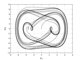
Figure 2: Trajectory of the Duffing oscillator with a sinusoidal forcing.

Props. 2 and 3 can also be applied to a hierarchical combination of more than two sub-systems. For Prop. 2, note that the serial connection of any number of 1-contracting sub-systems yields a 1-contracting system, so Prop. 2 may be applied to system where a 2-contracting sub-system feeds a serial connection of multiple 1-contracting sub-systems. For Prop. 3, it is clear from the proof that any number of sub-systems may be used, as long as each sub-system is NOB for any constant input.

Often we are given a dynamical system in the form

$$\dot{x}(t)=f(t,x),$$ (11)

and not necessarily the interconnection of two sub-systems. We may still be able to apply Props. 2 and 3 above if we can first decompose the given system as the serial connection of two sub-systems.

III-B Decomposing a given system as a serial connection of two sub-systems

An interesting and nontrivial problem is, given an $n$-dimensional dynamical system in the form (11), can the system be decomposed as the serial connection of two sub-systems? We address this question using a decomposition of $\mathbb{R}^{n}$ into two orthogonal subspaces, and a “uniform reducability” condition on the Jacobian of $f$.

We assume throughout that $f$ is $C^{1}$, that the solutions of (11) evolve on a convex state-space $\Omega\subseteq\mathbb{R}^{n}$, and that for any initial condition ${a\in\Omega}$, and time $t_{0}\geq 0$ a unique solution $x(t,t_{0},a)$ exists and satisfies $x(t,t_{0},a)\in\Omega$ for all $t\geq t_{0}$. Let $J(t,x):=\frac{\partial}{\partial x}f(t,x)$.

Consider an orthogonal decomposition of $\mathbb{R}^{n}$ into two linear subspaces $\mathcal{U}$ and $\mathcal{V}$ of dimensions $p$ and $q$, respectively, with $p,q\geq 1$ and $p+q=n$. Similar decompositions have been used in the context of contraction to subspaces [32] or manifolds [33]. The subspaces $\mathcal{U}$ and $\mathcal{V}$ are spanned by the columns of $U\in\mathbb{R}^{n\times p}$ and $V\in\mathbb{R}^{n\times q}$, respectively, which in turn are chosen such that

$$U^{T}U=I_{p},\;V^{T}V=I_{q},\;U^{T}V=0_{p\times q},\;UU^{T}+VV^{T}=I_{n}.$$ (12)

The next result provides a sufficient condition guaranteeing that (11) can be decomposed as the serial connection of two sub-systems.

Proposition 4.

Assume that any one of the following four equivalent conditions holds:

1. $V^{T}f(t,x)=V^{T}f(t,VV^{T}x)$ for all $t\in\mathbb{R}_{+}$, $x\in\Omega$;

2. $V^{T}J(t,x)U=0$ for all $t\in\mathbb{R}_{+}$, $x\in\Omega$;

3. $J(t,x)\mathcal{U}\subseteq\mathcal{U}$ for all $t\in\mathbb{R}_{+}$, $x\in\Omega$;

4. $J^{T}(t,x)\mathcal{V}\subseteq\mathcal{V}$ for all $t\in\mathbb{R}_{+}$, $x\in\Omega$.

Let $y^{1}:=V^{T}x$ and $y^{2}:=U^{T}x$. Then

$$\dot{y}^{1} =V^{T}f(t,Vy^{1}),$$

$$\dot{y}^{2} =U^{T}f(t,Uy^{2}+Vy^{1}).$$ (13)

Thus, any one of the four equivalent conditions guarantees that (11) can be decomposed as the serial interconnection of the two sub-systems in (4), where the output $Vy^{1}$ of the $q$-dimensional $y^{1}$ system is fed into the $p$-dimensional $y^{2}$ system. Note that conditions (c) and (d) are a form of “uniform reducibility” assumption on the Jacobian of the vector field or its transpose.

A typical case where the reducibility condition holds is when the dynamics is time-invariant and admits a first integral $H(x)=c^{T}x$, with $c\in\mathbb{R}^{n}\setminus\{0\}$. Then along solutions of the system, we have $0=\frac{d}{dt}H(x(t))=c^{T}f(x(t)),$ so condition (a) holds for $V={c}/{|c|}$.

Note also that $Vy^{1}=VV^{T}x=x-UU^{T}x,$ that is, the difference between $x$ and the (Euclidean norm) projection of $x$ on $\cal U$.

Proof.

We first show that the four conditions are equivalent. Suppose that condition (a) holds. Differentiating this condition with respect to $x$ gives $V^{T}J(t,x)=V^{T}J(t,VV^{T}x)VV^{T},$ and multiplying by $U$ on the right gives (b). To prove the converse implication, assume that (b) holds. Then

$$\begin{split}0&=\int_{0}^{1}V^{T}J(t,VV^{T}x+rUU^{T}x)UU^{T}x\mathrm{d}r\\ &=\int_{0}^{1}V^{T}\frac{\partial}{\partial r}f(t,VV^{T}x+rUU^{T}x)\mathrm{d}r\\ &=V^{T}f(t,x)-V^{T}f(t,VV^{T}x),\end{split}$$ (14)

where in the last equation we used (12). Thus, (b) implies (a). The equivalence of (b), (c), and (d) follows from (12). Now suppose that condition (a) holds. Let $y(t):=\begin{bmatrix}y^{1}(t)\\ y^{2}(t)\end{bmatrix}$, with $y^{1}:=V^{T}x$ and $y^{2}:=U^{T}x$. Then

$$\dot{y}^{1} =V^{T}f(t,x)$$

$$=V^{T}f(t,VV^{T}x)$$

$$=V^{T}f(t,Vy^{1}),$$ (15)

and

$$\dot{y}^{2} =U^{T}f(t,x)$$

$$=U^{T}f(t,UU^{T}x+VV^{T}x)$$

$$=U^{T}f(t,Uy^{2}+Vy^{1}),$$

and this completes the proof.

Example 2.

Consider the nonlinear system

$$\dot{x}=f(Lx),$$

where $L$ is the Laplacian of a weighted digraph. For example, if $f(y)=-y$ we get the linear consensus protocol, whereas if $f(y)=\begin{bmatrix}-\tanh(y_{1})&\dots&-\tanh(y_{n})\end{bmatrix}$ we get a form of a “bounded derivatives” consensus protocol.

Since $L1_{n}=0$, we can take $U:=\frac{1}{\sqrt{n}}1_{n}$, and let $V$ be as in (12). Then for $y^{1}:=V^{T}x$, $y^{2}:=U^{T}x$, we have

$$\dot{y}^{1}=V^{T}f(Lx)=V^{T}f(L(UU^{T}+VV^{T})x)=V^{T}f(LVy^{1}),$$

and

$$\dot{y}^{2}=(1/\sqrt{n})1_{n}^{T}f(Lx)=(1/\sqrt{n})1_{n}^{T}f(LVy^{1}).$$

The $(n-1)$-dimensional $y^{1}$ system describes the dynamics on the subspace orthogonal to the “consensus subspace” ${\cal U}=\operatorname{span}(1_{n})$. The dynamics of the $1$-dimensional $y^{2}$ system depends on $Vy^{1},$ that is, the difference between $x$ and its (Euclidean norm) projection on $\cal U$.

Remark 1.

Prop. 4 implies the well-known result that any LTI system $\dot{x}=Ax$, $A\in\mathbb{R}^{n\times n}$, with $n\geq 3$, may be decomposed into a serial interconnection of two sub-systems. If $A$ has a real eigenvalue $\lambda$, with a corresponding real eigenvector $u$, then $\mathcal{U}$ may be chosen as the subspace spanned by $u$. Otherwise, $A$ has a pair of complex conjugate eigenvalues $\alpha\pm j\beta$ and corresponding eigenvectors $u^{1}\pm ju^{2}$, where $\alpha\in\mathbb{R}$, $\beta\in\mathbb{R}\setminus\{0\}$, $u^{1}\in\mathbb{R}^{n}$, $u^{2}\in\mathbb{R}^{n}\setminus\{0\}$, and $j=\sqrt{-1}$. Let $\mathcal{U}:=\operatorname{span}(u^{1},u^{2})$. Then for any $z\in\mathcal{U}$,

$$Az=A(ru^{1}+su^{2})=(r\alpha+s\beta)u^{1}+(s\alpha-r\beta)u^{2},$$

so $A$ maps $\mathcal{U}$ to $\mathcal{U}$.

Remark 2.

The conditions in Prop. 4 are related to the existence of invariant sets of the dynamics (11) or of its corresponding variational equation. Indeed, pick two initial conditions $a,b\in\Omega$, an initial time $t_{0}:=0$, and let $z(t):=x(t,a)-x(t,b)$. Then

$$\dot{z}(t) =f(t,x(t,a))-f(t,x(t,b))$$

$$=\int_{0}^{1}\frac{\partial}{\partial r}f(t,rx(t,a)+(1-r)x(t,b))\mathop{}\!\mathrm{d}r$$

$$=\int_{0}^{1}J(t,rx(t,a)+(1-r)x(t,b))\mathop{}\!\mathrm{d}r\,z(t).$$

Combining this variational equation with condition (c) implies that if $a-b\in\cal U$ then $x(t,a)-x(t,b)\in\cal U$ for all $t\geq 0$.

If we assume, in addition, that $V^{T}f(t,0)=0$ for all $t\geq 0$ (this holds, for example, if $0$ is an equilibrium of (11) for all $t\geq 0$) then condition (a) gives

$$V^{T}f(t,UU^{T}x)=V^{T}f(t,VV^{T}UU^{T}x)=V^{T}f(t,0)\equiv 0,$$

and this implies that $f(t,\mathcal{U})\subseteq\mathcal{U},$ i.e. $\mathcal{U}$ is an invariant set of the dynamics.

The next result demonstrates an application of Prop. 4 to a system with a feedback form.

Corollary 1.

Consider an $(n+m)$-dimensional system:

$$\dot{x} =g(z),$$ (16)

$$\dot{z} =h(Mx,z),$$

where $x\in\mathbb{R}^{n}$, $z\in\mathbb{R}^{m}$, and $M\in\mathbb{R}^{k\times n}$. Suppose that there exist $U\in\mathbb{R}^{n\times p}$ and $V\in\mathbb{R}^{n\times(n-p)}$ as in (12) such that

$$MU=0.$$ (17)

Define $y^{1}:=V^{T}x$, $y^{2}:=z$, and $y^{3}:=U^{T}x$. Then

$$\dot{y}^{1} =V^{T}g(y^{2}),$$

$$\dot{y}^{2} =h(MVy^{1},y^{2}),$$

$$\dot{y}^{3} =U^{T}g(y^{2}).$$ (18)

Note that this implies a decomposition into an $(n+m-p)$-dimensional sub-system with state $\begin{bmatrix}y^{1}\\ y^{2}\end{bmatrix}$, whose output $g(y^{2})$ is fed into the $p$-dimensional $y^{3}$ sub-system. Note also that if $\operatorname{rank}(M)<n$ then we can always find $U,V$ satisfying condition (17).

Proof.

Define matrices $\tilde{U}\in\mathbb{R}^{(n+m)\times p}$ and $\tilde{V}\in\mathbb{R}^{(n+m)\times(n+m-p)}$ by $\tilde{U}:=\begin{bmatrix}U\\ 0\end{bmatrix}$, $\tilde{V}:=\begin{bmatrix}V&0\\ 0&I\end{bmatrix}.$ The Jacobian of (16) is

$$J(x,z)=\begin{bmatrix}0&\frac{\partial}{\partial z}g(z)\\ \frac{\partial}{\partial x}h(Mx,z)M&\frac{\partial}{\partial z}h(Mx,z)\end{bmatrix},$$ (19)

so $J(x,z)\begin{bmatrix}U\\ 0\end{bmatrix}=0$ for all $x,z$. Thus, $J$ maps the subspace ${\cal\tilde{U}}$ corresponding to $\tilde{U}$ to itself. By Prop. 4, the system can be decomposed as the serial connection of two sub-systems by defining $\tilde{y}^{1}:=\tilde{V}^{T}\begin{bmatrix}x\\ z\end{bmatrix}$ and $\tilde{y}^{2}:=\tilde{U}^{T}\begin{bmatrix}x\\ z\end{bmatrix}$, that is, $\tilde{y}^{1}=\begin{bmatrix}V^{T}x\\ z\end{bmatrix}$ and $\tilde{y}^{2}:=U^{T}x$. Computing the dynamics of $y^{1}$ and $y^{2}$ yields (1).

Example 3.

Consider the second-order consensus system [34]:

$$\dot{x} =v,$$

$$\dot{v} =u,$$ (20)

with

$$u=f(\beta Lx+\alpha Lv).$$

Here $x\in\mathbb{R}^{n}$, $x_{i}$ describes the (scalar) location of agent $i$, $v_{i}$ is the velocity of agent $i$, $L$ is the Laplacian of a weighted digraph, and $\alpha,\beta>0$. The goal is to drive both the $x_{i}$s and the $v_{i}$s to consensus, that is, $x(t)\to c_{1}1_{n}$, $v(t)\to c_{2}1_{n}$ for some constants $c_{1},c_{2}$. The nonlinear function can be for example $f(y)=-y$ or $f(y)=-\tanh(y)$.

This system has the form described in Corollary 1 with $z=v$, $m=n$, $g(z)=z$, $M=\beta L$, and $h(Mx,z)=f(Mx+\alpha Lz)$. We can thus take $U=\frac{1}{\sqrt{n}}1_{n}$, and a $V\in\mathbb{R}^{n\times(n-1)}$ such that (12) holds. Then for $y^{1}:=V^{T}x$, $y^{2}:=v$, and $y^{3}:=\frac{1}{\sqrt{n}}1_{n}^{T}x$, we get

$$\dot{y}^{1} =V^{T}y^{2},$$

$$\dot{y}^{2} =f(\beta LVy^{1}+\alpha Lv),$$

$$\dot{y}^{3} =U^{T}y^{2}.$$

The first two equations form a $(2n-1)$ dimensional system, and the third describes the dynamics of $1_{n}^{T}x$.

In the next subsection, we combine Props. 2 and 3 with the reducibility condition to guarantee the well-ordered behaviour of the time-invariant system

$$\dot{x}=f(x).$$ (21)

We assume throughout that $f$ is $C^{1}$ and that the trajectories evolve on a convex set $\Omega\subseteq\mathbb{R}^{n}$. Let $J(x):=\frac{\partial}{\partial x}f(x)$.

III-C Conditions for well-ordered behaviour of $\dot{x}=f(x)$

The next result provides a sufficient condition for NOB that is based on 2-contraction on a certain subspace. As shown in Example 4 below, this is weaker than requiring 2-contraction on the entire state-space.

Proposition 5.

Suppose that the decomposition condition in Prop. 4 holds for (21) with $\mathcal{U}$ a one-dimensional subspace, i.e. $p=1$, and that there exists a matrix measure $\mu$ such that

$$\mu\left((V^{T})^{(2)}J^{[2]}(x)V^{(2)}\right)\leq-\eta<0,\text{ for all }x\in\Omega.$$ (22)

Then (21) is NOB.

Proof.

We know that for $y^{1}:=V^{T}x$ and $y^{2}:=U^{T}x$, we have $\dot{y}^{1}=V^{T}f(Vy^{1}),$ and $\dot{y}^{2}=U^{T}f(Uy^{2}+Vy^{1})$. The Jacobian of the $y^{1}$ system is $V^{T}J(Vy^{1})V$, and combining this with (II) and (22) implies that the $y^{1}$ system is 2-contracting and thus NOB. The $y^{2}$ system is one-dimensional and thus NOB for any constant input. Applying Prop. 3 completes the proof.

Note that the existence of a one-dimensional invariant subspace is quite common in various systems, e.g. in models for synchronization, where the synchronized state (i.e., $x_{1}=\dots=x_{n}$) is invariant, see also the examples in Section IV.

It is instructive to demonstrate Prop. 5 in the case of an LTI system.

Example 4.

Consider the LTI system

$$\dot{x}(t)=Ax(t).$$ (23)

In this case, the decomposition condition is $A\,{\mathcal{U}}\subseteq\mathcal{U}$. Let $T$ be the $n\times n$ matrix

$$T:=\begin{bmatrix}V^{T}\\ U^{T}\\ \end{bmatrix}.$$ (24)

Then $T^{-1}=\begin{bmatrix}V&U\end{bmatrix}$, and

$$TAT^{-1}=\begin{bmatrix}U^{T}AU&U^{T}AV\\ 0&V^{T}AV\end{bmatrix}.$$ (25)

Thus, $TAT^{-1}$ is reducible. The spectrum of $A$ is the union of the real scalar $U^{T}AU$ and the spectrum of $V^{T}AV$. Since $V^{T}AV$ is 2-contracting, it has no pure imaginary eigenvalues, so $A$ has no pure imaginary eigenvalues. Thus, (23) has no non-trivial periodic trajectories.

It is important to note that the eigenvalue $U^{T}AU$ of $TAT^{-1}$, and thus of $A$, can be arbitrarily large, so $A$ is not necessarily $2$-contracting in the entire state-space.

Roughly speaking, Prop. 5 requires that $\mathcal{U}$ is one-dimensional and that the system is 2-contracting on $\mathcal{V}$, and proves that such a configuration is NOB. By requiring that the system is instead 1-contracting on $\mathcal{U}$ (no longer necessarily one-dimensional), we now derive a stronger result, namely that every bounded trajectory of the overall system converges to an equilibrium point. Example 5 below shows that these conditions do not imply that the system is 2-contracting on the entire state-space.

Proposition 6.

Suppose that the decomposition condition in Prop. 4 holds, and that there exists a matrix measure $\mu$ such that

$$\mu((V^{T})^{(2)}J^{[2]}(x)V^{(2)})\leq-\eta<0$$ (26)

and

$$\mu(U^{T}J(x)U)\leq-\beta<0$$ (27)

for all $x\in\Omega$. Then every bounded trajectory of (21) converges to an equilibrium point.

Proof.

For $y^{1}:=V^{T}x$ and $y^{2}:=U^{T}x$, we have $\dot{y}^{1}=V^{T}f(Vy^{1}),$ and $\dot{y}^{2}=U^{T}f(Uy^{2}+Vy^{1})$. The Jacobian of the $y^{1}$ system is $V^{T}J(Vy^{1})V$, and combining this with (II) and (26) implies that the $y^{1}$ system is 2-contracting. The Jacobian of the $y^{2}$ system is $U^{T}J(Vy^{1}+Uy^{2})U$, so (27) implies that the $y^{2}$ system is 1-contracting. Applying Prop. 2 completes the proof.

Again, it is instructive to demonstrate Prop. 6 in the case of an LTI system.

Example 5.

Consider the LTI system (23). The decomposition condition implies that $V^{T}AU=0$, so (25) holds. Eq. (27) implies that all the eigenvalues of $U^{T}AU$ have a negative real part. Eq. (26) implies that $V^{T}AV$ has no pure imaginary eigenvalue. We conclude that the spectrum of $A$ has no pure imaginary eigenvalues. Thus, any bounded trajectory of the LTI converges to an equilibrium point.

Note that the conditions do not imply that the overall system is 2-contracting on the entire state-space. Consider for example the LTI system (23) with $A=\operatorname{diag}(2,-3,-1,-1)$. Let $U:=\begin{bmatrix}0\\ I_{2}\end{bmatrix},V:=\begin{bmatrix}I_{2}\\ 0\end{bmatrix}.$ Then, for any monotonic norm $\mu(U^{T}AU)\leq-1$ and $\mu((V^{T})^{(2)}A^{[2]}V^{(2)})=-1$. The decomposition condition also holds. However, the maximal eigenvalue of $A^{[2]}$ is one, so the system is not 2-contracting on the entire state-space for any norm.

IV Applications

We describe two simple applications of the theoretical results. We will make use of the following fact (see, e.g. [35]). If $A\in\mathbb{R}^{3\times 3}$ then

$$A^{[2]}=\begin{bmatrix}a_{11}+a_{22}&a_{23}&-a_{13}\\ a_{32}&a_{11}+a_{33}&a_{12}\\ -a_{31}&a_{21}&a_{22}+a_{33}\end{bmatrix}.$$ (28)

Our first application is a 3D system with two agents.

Corollary 2.

Consider the system

$$\dot{x}_{1} =f(x_{1},x_{2}),$$

$$\dot{x}_{2} =x_{3}-x_{1},$$ (29)

$$\dot{x}_{3} =g(x_{3},x_{2}).$$

Assume that

$$\frac{\partial}{\partial x_{1}}f(x_{1},x_{2})=\frac{\partial}{\partial x_{3}}g(x_{3},x_{2})\leq-\delta<0\text{ for all }x,$$ (30)

and that the trajectories evolve on a convex and compact set. Then every trajectory of (2) converges to an equilibrium point.

Here $x_{1}$ and $x_{3}$ may represent the state of two “agents”, and $x_{2}$ evolves according to the difference between the agent states. A typical example is a system describing the interconnection of two synchronous generators, that interact via an integral of the difference between their frequencies (i.e. the relative phase angle) [36]. In the control theory community, such models are often called network reduced power systems.

Proof.

The Jacobian of (2) is $J=\begin{bmatrix}\frac{\partial}{\partial x_{1}}f&\frac{\partial}{\partial x_{2}}f&0\\ -1&0&1\\ 0&\frac{\partial}{\partial x_{2}}g&\frac{\partial}{\partial x_{3}}g\end{bmatrix}.$ Consider the orthogonal decomposition generated by the matrices

$$U:=\frac{1}{\sqrt{2}}\begin{bmatrix}1\\ 0\\ 1\end{bmatrix},\quad V:=\frac{1}{\sqrt{2}}\begin{bmatrix}0&1\\ \sqrt{2}&0\\ 0&-1\\ \end{bmatrix}.$$

Then $V^{T}JU=(1/2)\begin{bmatrix}0\\ \frac{\partial}{\partial x_{1}}f-\frac{\partial}{\partial x_{3}}g\end{bmatrix},$ and (30) gives $V^{T}JU=0$. Additionally, $V^{(2)}=\begin{bmatrix}-1&0&-1\end{bmatrix}^{T}$, and

$$J^{[2]}=\begin{bmatrix}\frac{\partial}{\partial x_{1}}f&1&0\\ \frac{\partial}{\partial x_{2}}g&\frac{\partial}{\partial x_{1}}f+\frac{\partial}{\partial x_{3}}g&\frac{\partial}{\partial x_{2}}f\\ 0&-1&\frac{\partial}{\partial x_{3}}g\end{bmatrix},$$

so (30) yields $(V^{T})^{(2)}J^{[2]}V^{(2)}=\frac{\partial}{\partial x_{1}}f+\frac{\partial}{\partial x_{3}}g\leq-2\delta<0$, and the 2D sub-system is 2-contracting. Similarly, $U^{T}JU\leq-2\delta<0$ and the scalar sub-system is 1-contracting. Applying Prop. 6 completes the proof of Corollary 2.

Our second application describes a system of three “synchronizing agents”.

Corollary 3.

Consider the system:

$$\dot{x}_{1} =f(x_{1}-x_{2})+f(x_{1}-x_{3}),$$

$$\dot{x}_{2} =g(x_{2}-x_{1})+g(x_{2}-x_{3}),$$ (31)

$$\dot{x}_{3} =h(x_{3}-x_{2})+h(x_{3}-x_{1}),$$

where $f,g,h:\mathbb{R}\to\mathbb{R}$ are $C^{1}$. Suppose that the trajectories evolve on a compact and convex set $\Omega$ and that

$$f^{\prime}(p)+g^{\prime}(-p)+f^{\prime}(q)+h^{\prime}(-q)+g^{\prime}(q-p)+h^{\prime}(p-q)\leq-\eta<0$$ (32)

for any $p,q\in\mathbb{R}$. Then (3) is NOB.

Proof.

Let $x_{ij}:=x_{i}-x_{j}$. The Jacobian $J(x)$ of (3) is

$$\begin{bmatrix}f^{\prime}(x_{12})+f^{\prime}(x_{13})&-f^{\prime}(x_{12})&-f^{\prime}(x_{13})\\ -g^{\prime}(x_{21})&g^{\prime}(x_{21})+g^{\prime}(x_{23})&-g^{\prime}(x_{23})\\ -h^{\prime}(x_{31})&-h^{\prime}(x_{32})&h^{\prime}(x_{32})+h^{\prime}(x_{31})\end{bmatrix},$$

and using (28) implies that

$$J^{[2]}(x)=\left[\begin{smallmatrix}J_{11}(x)+J_{22}(x)&-g^{\prime}(x_{23})&f^{\prime}(x_{13})\\ -h^{\prime}(x_{32})&J_{11}(x)+J_{33}(x)&-f^{\prime}(x_{12})\\ h^{\prime}(x_{31})&-g^{\prime}(x_{21})&J_{22}(x)+J_{33}(x)\end{smallmatrix}\right].$$

Let $U:=\frac{1}{\sqrt{3}}\begin{bmatrix}1\\ 1\\ 1\end{bmatrix}$, $V:=\frac{1}{\sqrt{6}}\begin{bmatrix}2&0\\ -1&-\sqrt{3}\\ -1&\sqrt{3}\end{bmatrix}$. Then $J(x)U=0$ for all $x$, so the reducibility condition holds. A calculation gives $V^{(2)}=\frac{1}{\sqrt{3}}\begin{bmatrix}-1&1&-1\end{bmatrix}^{T}$, and

$$(V^{T})^{(2)} J^{[2]})(x)V^{(2)}=f^{\prime}(x_{12})+f^{\prime}(x_{13})$$

$$+g^{\prime}(x_{21})+g^{\prime}(x_{23})+h^{\prime}(x_{31})+h^{\prime}(x_{32}).$$

Combining this with (32) implies that all the conditions in Prop. 5 hold. This completes the proof of Corollary 3.

V Conclusion

An important topic in systems theory is analyzing an interconnected system based on the properties of the sub-systems and the interconnection network. In this context, an important advantage of contracting systems is that various interconnections of such systems yield a contracting system.

We analyzed the serial interconnection of $k$-contracting systems, with $k\in\{1,2\}$. Our results guarantee NOB and, under stronger assumptions, that every bounded solution converges to an equilibrium (that is not necessarily unique). To apply these results to a wider set of systems, we also derived a reducibility condition guaranteeing that a given system can be decomposed as the serial connection of two systems.

Prop. 4 provides a sufficient condition for decomposing a system as the serial connection of two sub-systems based on a decomposition of $\mathbb{R}^{n}$ into two subspaces. It may be of interest to extend this result using more general decompositions of $\mathbb{R}^{n}$.

Our reducibility condition is restrictive and not robust to small perturbations in the dynamics. Another topic for further research is to apply our results to a system $\dot{x}=f(x)$ that does not satisfy the reducibility condition using the following scheme: (1) approximate $f$ using a vector field $g$ that does satisfy the reducibility condition; (2) analyze the dynamics $\dot{y}=g(y)$ using the tools developed here; and (3) use comparison principles for ODEs [37] to show that the results for the $y$-system also hold for the original $x$-system. These topics are currently under study.

References

• [1] W. Lohmiller and J.-J. E. Slotine, “On contraction analysis for non-linear systems,” Automatica, vol. 34, pp. 683–696, 1998.
• [2] G. Russo, M. di Bernardo, and E. D. Sontag, “Global entrainment of transcriptional systems to periodic inputs,” PLOS Computational Biology, vol. 6, p. e1000739, 2010.
• [3] A. Pavlov, N. van de Wouw, and H. Nijmeijer, “Frequency response functions and Bode plots for nonlinear convergent systems,” in Proc. 45th IEEE Conf. on Decision and Control, 2006, pp. 3765–3770.
• [4] A. V. Pavlov, N. van de Wouw, and H. Nijmeijer, Uniform Output Regulation of Nonlinear Systems: A Convergent Dynamics Approach.   Boston, MA: Birkhauser, 2006.
• [5] Z. Aminzare and E. D. Sontag, “Contraction methods for nonlinear systems: A brief introduction and some open problems,” in Proc. 53rd IEEE Conf. on Decision and Control, Los Angeles, CA, 2014, pp. 3835–3847.
• [6] G. Russo, M. di Bernardo, and E. Sontag, “A contraction approach to the hierarchical analysis and design of networked systems,” IEEE Trans. Automat. Control, vol. 58, no. 5, pp. 1328–1331, 2013.
• [7] C. Wu, I. Kanevskiy, and M. Margaliot, “$k$-order contraction: theory and applications,” 2020, submitted. [Online]. Available: https://arxiv.org/abs/2008.10321
• [8] I. R. Manchester and J.-J. E. Slotine, “Combination properties of weakly contracting systems,” 2014. [Online]. Available: https://arxiv.org/abs/1408.5174
• [9] J. S. Muldowney, “Compound matrices and ordinary differential equations,” The Rocky Mountain J. Math., vol. 20, no. 4, pp. 857–872, 1990.
• [10] M. Y. Li and J. S. Muldowney, “On R. A. Smith’s autonomous convergence theorem,” Rocky Mountain J. Math., vol. 25, no. 1, pp. 365–378, 1995.
• [11] J. W. Simpson-Porco and F. Bullo, “Contraction theory on Riemannian manifolds,” Systems Control Lett., vol. 65, pp. 74–80, 2014.
• [12] S. Jafarpour, P. Cisneros-Velarde, and F. Bullo, “Weak and semi-contraction for network systems and diffusively-coupled oscillators,” IEEE Trans. Automat. Control, 2021, to appear.
• [13] M. Margaliot, T. Tuller, and E. Sontag, “Checkable conditions for contraction after small transients in time and amplitude,” in Feedback Stabilization of Controlled Dynamical Systems: In Honor of Laurent Praly, N. Petit, Ed.   Cham, Switzerland: Springer International Publishing, 2017, pp. 279–305.
• [14] M. di Bernardo, D. Liuzza, and G. Russo, “Contraction analysis for a class of nondifferentiable systems with applications to stability and network synchronization,” SIAM J. Control Optim., vol. 52, no. 5, pp. 3203–3227, 2014.
• [15] P. Wensing and J.-J. Slotine, “Beyond convexity-contraction and global convergence of gradient descent,” PLoS One, vol. 15, no. 8, pp. 1–29, 2020.
• [16] A. Douady and J. Oesterlé, “Dimension de Hausdorff des attracteurs,” C. R. Acad. Sc. Paris, vol. 290, pp. 1135–1138, 1980.
• [17] N. Kuznetsov and V. Reitmann, Attractor Dimension Estimates for Dynamical Systems: Theory and Computation. Dedicated to Gennady Leonov.   Cham, Switzerland: Springer, 2021.
• [18] M. Margaliot and E. D. Sontag, “Revisiting totally positive differential systems: A tutorial and new results,” Automatica, vol. 101, pp. 1–14, 2019.
• [19] R. Katz, M. Margaliot, and E. Fridman, “Entrainment to subharmonic trajectories in oscillatory discrete-time systems,” Automatica, vol. 116, p. 108919, 2020.
• [20] C. Wu, R. Pines, M. Margaliot, and J.-J. Slotine, “Generalization of the multiplicative and additive compounds of square matrices and contraction in the Hausdorff dimension,” 2021, submitted. [Online]. Available: http://arxiv.org/abs/2012.13441
• [21] C. Wu and M. Margaliot, “Diagonal stability of discrete-time $k$-positive linear systems with applications to nonlinear systems,” 2020. [Online]. Available: https://arxiv.org/abs/2102.02144
• [22] E. Bar-Shalom and M. Margaliot, “Compound matrices in systems and control theory,” in Proc. 60th IEEE Conf. on Decision and Control, 2021, accepted.
• [23] R. A. Horn and C. R. Johnson, Matrix Analysis, 2nd ed.   Cambridge University Press, 2013.
• [24] S. Winitzki, Linear Algebra via Exterior Products.   lulu.com, 2010.
• [25] W. A. Coppel, Stability and Asymptotic Behavior of Differential Equations.   Boston, MA: D. C. Heath, 1965.
• [26] L. A. Sanchez, “Cones of rank 2 and the Poincaré-Bendixson property for a new class of monotone systems,” J. Diff. Eqns., vol. 246, no. 5, pp. 1978–1990, 2009.
• [27] H. L. Smith, “Systems of ordinary differential equations which generate an order preserving flow,” SIAM Rev., vol. 30, pp. 87–113, 1988.
• [28] E. Weiss and M. Margaliot, “A generalization of linear positive systems with applications to nonlinear systems: Invariant sets and the Poincaré-Bendixson property,” Automatica, vol. 123, p. 109358, 2021.
• [29] M. Y. Li and J. S. Muldowney, “Global stability for the SEIR model in epidemiology,” Math. Biosciences, vol. 125, no. 2, pp. 155–164, 1995.
• [30] C. C. Pugh, “An improved closing lemma and a general density theorem,” American J. Math., vol. 89, no. 4, pp. 1010–1021, 1967.
• [31] E. P. Ryan and E. D. Sontag, “Well-defined steady-state response does not imply CICS,” Systems Control Lett., vol. 55, pp. 707–710, 2006.
• [32] Q. C. Pham and J.-J. Slotine, “Stable concurrent synchronization in dynamic system networks,” Neural Networks, vol. 20, no. 1, pp. 62–77, 2007.
• [33] I. R. Manchester and J.-J. E. Slotine, “Control contraction metrics: Convex and intrinsic criteria for nonlinear feedback design,” IEEE Trans. Automat. Control, vol. 62, no. 6, pp. 3046–3053, 2017.
• [34] W. Yu, G. Chen, and M. Cao, “Some necessary and sufficient conditions for second-order consensus in multi-agent dynamical systems,” Automatica, vol. 46, no. 6, pp. 1089–1095, 2010.
• [35] B. Schwarz, “Totally positive differential systems,” Pacific J. Math., vol. 32, no. 1, pp. 203–229, 1970.
• [36] P. Kundur, Power System Stability and Control.   McGraw-Hill Education, 1994.
• [37] J. Szarski, Differential Inequalities.   Instytut Matematyczny Polskiej Akademi Nauk, 1965.