Iterated star-triangle transformation
on inhomogeneous 2D Ising lattices

Abstract

We consider infinite or periodic 2D triangular Ising lattices with arbitrary positive or negative nearest-neighbor couplings $K_{i}(\vec{r})$, where $\vec{r}$ and $i$ indicate the bond position and orientation, respectively. Iterative application of the star-triangle transformation to an initial lattice $\mathcal{T}(0)$ with a set of couplings $\{K_{i}^{(0)}(\vec{r})\}$ generates a sequence of lattices $\mathcal{T}(n)$, for $n=1,2,\ldots,$ with couplings $\{K_{i}^{(n)}(\vec{r})\}$. When $\mathcal{T}(0)$ includes sufficiently strongly frustrated plaquettes, complex couplings will appear. We show that, nevertheless, the variables $1/\sinh 2K_{i}^{(n)}\!(\vec{r})$ remain confined to the union ${\mathbb{R}}\cup{\rm i}{\mathbb{R}}$ of the real and the imaginary axis. The same holds for a lattice with free boundaries, provided we distinguish between “receding” and “advancing” boundaries, the latter having degrees of freedom that must be fixed by an appropriately chosen protocol. This study establishes a framework for future analytic and numerical work on such frustrated Ising lattices.

1 Introduction

We consider an Ising model with nearest-neighbor interactions on a triangular lattice. Figure 1 shows on the left a local configuration where a triangle of spins $\sigma_{1}$, $\sigma_{2}$, and $\sigma_{3}$ interacts via three nearest-neighbor couplings $K_{1},K_{2},$ and $K_{3}$. The expression for the partition function of this lattice may be transformed in various ways. It is in particular possible to “decorate” the lattice by inserting a central spin $\sigma_{0}$ such that the triangle of couplings is replaced with a three-legged star of couplings $p_{1}$, $p_{2}$, and $p_{3}$ linking the central spin to the three others, as shown on the right of figure 1. The $p_{j}$ have well-defined expressions in terms of the $K_{i}$ (with $i,j=1,2,3$), and inversely. The relevant formulas, of which a derivation may be found in Syozi [1], will be displayed in section 2.

The decoration transformation is fully reversible: we may “decimate” the central spin in a star of pairwise interacting spins and thereby recover the original triangle. Applied either way, the operation is referred to as the star-triangle (ST) transformation.

Figure 1: The star-triangle transformation. The coupling strengths $K_{i}$ of the triangle sides may be transformed into the $p_{j}$ of the star legs and vice versa.

A homogeneous  triangular or hexagonal lattice is one in which the couplings depend only on the orientation $i$ of the bonds. In the study of the two-dimensional (2D) Ising model the ST transformation for the homogeneous isotropic case ($K_{i}=K$ and $p_{i}=p$ for all $i=1,2,3$) appears in Onsager [2] and in Wannier [3]. The homogeneous but anisotropic case (three different $K_{i}$ and $p_{i}$) seems to have been first exhibited by Houtappel [4]. This author combined the ST transformation with a high/low temperature duality and established the critical surfaces of the triangular and hexagonal Ising lattices in the $K_{1}K_{2}K_{3}$ and $p_{1}p_{2}p_{3}$ parameter space, respectively. In one important line of development the ST transformation and its generalization to the Yang-Baxter equations have become a cornerstone in the study of integrable models (see, e.g., Perk and Au-Yang [5, 6]).

1.1 Star-triangle (ST) evolution

The focus of our work is on triangular and hexagonal lattices with nearest-neighbor couplings $\{K_{i}(\vec{r})\}$ that are inhomogeneous, i.e., that vary with the spatial position $\vec{r}$. Let us consider the triangular lattice $\mathcal{T}(0)$ made up of the thin solid lines in figure 2a and whose couplings we will denote by $\{K_{i}^{(0)}(\vec{r})\}$. We will suppose that this lattice has no boundaries (it is infinite or periodic in both directions). We start by partitioning this lattice into upward pointing triangles. Upon applying the ST transformation independently to each of these triangles we generate a collection of upward pointing stars that together constitute a hexagonal lattice, to be called $\mathcal{H}(0)$. It is made up of the thick dashed lines in figure 2a and has been reproduced in figure 2b. We now partition this lattice in a different way, namely into downward-pointing stars, and apply the ST transformation to those. This generates a collection of downward-pointing triangles that together constitute a new triangular lattice that we will call $\mathcal{T}(1)$, and that is made up of the heavy solid lines in figure 2b. The lattices $\mathcal{T}(0)$ and $\mathcal{T}(1)$ differ by a translation but are geometrically identical. If $\mathcal{T}(0)$ is homogeneous with couplings $K_{1},K_{2},$ and $K_{3}$, then $\mathcal{T}(1)$ will also be homogeneous and have the same couplings. However, if $\mathcal{T}(0)$ is inhomogeneous, then so will $\mathcal{T}(1)$ be, but with a different set $\{K_{i}^{(1)}(\vec{r})\}$ of coupling strengths.

We will view the mapping from $\mathcal{T}(0)$ to $\mathcal{T}(1)$, via the intermediate lattice $\mathcal{H}(0)$, as one iteration of the ST transformation, composed of two steps. Successive iterations generate the sequence

$$\mathcal{T}(0) \,\mapsto \mathcal{H}(0) \,\mapsto \mathcal{T}(1) \,\mapsto \mathcal{H}(1) \,\mapsto \,\mapsto \mathcal{T}(n) \,\mapsto \mathcal{H}(n) \,\mapsto$$ … …, (1.1)

in which each lattice is characterized by its set of couplings, $\{K_{i}^{(n)}(\vec{r})\}$ or $\{p_{i}^{(n)}(\vec{r})\}$, for $n=0,1,2,\ldots$, and where each step, $\mathcal{T}\mapsto\mathcal{H}$ or $\mathcal{H}\mapsto\mathcal{T}$, is followed by a repartitioning of the stars or of the triangles, respectively. We will refer to sequence (1.1) as the ST evolution  of the initial lattice. It is an inhomogeneity-driven  mapping in the space of nearest-neighbor Hamiltonians on the triangular lattice.

Figure 2: (a) Thin solid lines: lattice $\mathcal{T}(0)$. Thick dashed lines: lattice $\mathcal{H}(0)$ obtained from $\mathcal{T}(0)$ by ST transformation. (b) The same lattice $\mathcal{H}(0)$ and, in thick solid lines, lattice $\mathcal{T}(1)$ obtained from it by ST transformation.

1.2 Applications

ST evolution has led to various analytical and numerical applications. It was introduced by the author et al. [7, 8], who exploited it to construct an exact renormalization transformation in “real space” of the 2D Ising model. Their particular application was based on three couplings $K_{i}^{(n)}(\vec{r})$ that for fixed $i$ vary smoothly with the spatial position $\vec{r}$ and with the iteration index $n$. ST evolution then becomes a continuous flow described by a set of three coupled nonlinear partial differential equations. Subsequently the flow in the critical surface was studied in greater detail [9], and similar ST evolution equations were formulated for the $d$-dimensional Gaussian model [10, 11, 12], where stars have $d+1$ legs and triangles are replaced with $d$-simplices.

ST evolution has yielded new results in particular for the class of semi-infinite 2D Ising lattices. Under this evolution the boundary magnetization and the boundary-spin correlation of such lattices couple only to themselves and may be calculated numerically exactly or, in certain cases, analytically [13, 14, 15, 16, 17, 18, 19, 20, 21]. Furthermore, several of the techniques developed in this context have been transposed to 1D quantum chains, whether they be nonrandom or disordered [22, 23, 24, 25, 26, 27, 28, 29]. Review articles on these semi-infinite models are due to Iglói et al. [30] and Pelizzola [31].

1.3 This work

The present work is motivated by the absence, so far, of applications of the ST transformation to frustrated Ising lattices, and notably to Ising spin glasses. We investigate here the behavior of ST evolution for initial triangular lattices $\mathcal{T}(0)$ having a mixture of ferromagnetic (positive) and antiferromagnetic (negative) coupling strengths. Such initial conditions allow for frustration, which will cause complex couplings to be generated in the lattices $\mathcal{T}(1)$, ${\mathcal{T}}(2),\ldots$. We establish rules that are universally obeyed by the ST evolution of complex couplings. The central result is that for a system without boundaries (i.e., which is infinite or periodic in both directions) the variables $S_{i}^{(n)}(\vec{r})=1/\sinh 2K_{i}^{(n)}(\vec{r})$ remain confined to the union of the real and the imaginary axis. An analogous statement holds for the intermediate hexagonal lattices. For a system with boundaries the above statements, while remaining essentially valid, have to be formulated more carefully and require separate proof.

We are not dealing in this work with an application to any specific system. We believe that the rules that we will describe are interesting in their own right and we expect them to play a role in future applications of the ST transformation to specific frustrated lattices.

This paper is organized as follows. In Section 2 we recall the basic ST transformation formula and state the main theorem, applicable to systems without a boundary. In Section 3 we define the concept of the “color” of a bond. We derive rules for the evolution of the colors under iteration of the ST transformation and, relying on these rules, prove the main theorem. In Section 4 we consider lattices with boundaries and are led to distinguish between “advancing” and “receding” ones. Stars and triangles located at the boundaries may be incomplete, that is, they may miss legs or sides, and we provide the required modifications of the ST transformation formulas for those cases. At advancing boundaries the necessity of a “protocol” appears, as discussed in section 4.3. In Section 5 we investigate the ST evolution of the bond colors in the presence of boundaries and prove the relevant modified theorems. In Section 6 we present our conclusions.

2 The star-triangle transformation formula

When no confusion can arise we will drop the iteration index $n$ and the spatial position $\vec{r}$, and we will write $\{K_{1},K_{2},K_{3}\}$ for an arbitrary triplet of couplings under consideration. Analogous notation will be used for the coupling strengths on the intermediate hexagonal lattices.

We will now connect the coupling strengths $p_{j}$ of three star legs to the $K_{i}$ of the three corresponding triangle sides, with $i,j=1,2,3$ indicating the bond orientations according to figure 1.

When dealing with a star $\{p_{1},p_{2},p_{3}\}$ we will let $S_{i}$ and $C_{i}$ stand for

$$S_{i}=\sinh 2p_{i}\,,\qquad C_{i}=\cosh 2p_{i}\,,\qquad i=1,2,3;$$ (2.1)

and, for reasons to become clear below, when dealing with a triangle $\{K_{1},K_{2},K_{3}\}$ we will let these same variables stand for

$$S_{i}=1/\sinh 2K_{i}\,,\qquad C_{i}=\coth 2K_{i}\,,\qquad i=1,2,3.$$ (2.2)

We may therefore denote a bond by $(S_{i},C_{i})$ without specifying if it is a star leg $p_{i}$ or a triangle side $K_{i}$. Definitions (2.1) and (2.2) both lead to the relation

$$C_{i}^{2}-S_{i}^{2}=1,\qquad i=1,2,3.$$ (2.3)

Let a triplet of ingoing  bonds $(S_{j},C_{j})$, with $j=1,2,3$, be subjected to the ST transformation such that it produces a triplet of outgoing  bonds $(S_{i}^{\,\prime},C_{i}^{\,\prime})$ with $i=1,2,3$. After a somewhat tedious calculation one finds that the ST transformation takes the form [1]

$$S_{i}^{\,\prime}=\frac{F^{1/2}}{S_{j}S_{k}}\,,\qquad C_{i}^{\,\prime}=\frac{C_{i}+C_{j}C_{k}}{S_{j}S_{k}}\,,\qquad i,j,k\,\mbox{ cyclic,}$$ (2.4)

in which $F$ is given by

$$F=2+S_{1}^{2}+S_{2}^{2}+S_{3}^{2}+2C_{1}C_{2}C_{3}\,$$ (2.5)

and one may verify that again

$$C_{i}^{\,\prime\,2}-S_{i}^{\,\prime\,2}=1,\qquad i=1,2,3.$$ (2.6)

The advantage of equations (2.4)-(2.6) is that they are valid for both the step $\mathcal{T}\mapsto\mathcal{H}$ and $\mathcal{H}\mapsto\mathcal{T}$, which was the reason for definitions (2.1)-(2.2).

The ST transformation leaves the partition function invariant up to a multiplicative constant $G$, whose expression in terms of the $S_{i}$ and $C_{i}$ does not concern us here. In equation (2.4) the sign of the square root $F^{1/2}$ may be chosen according to an arbitrary convention.

3 Bond color evolution

We consider now the sequence of lattices (1.1) generated from a given initial lattice $\mathcal{T}(0)$. The basic result of this work refers to a lattice without boundaries, that is, which is infinite or periodic in both directions. It may be stated as follows.

Theorem 1. Let a triangular lattice $\mathcal{T}(0)$ without boundaries have initial couplings $K_{i}^{(0)}(\vec{r})$ that are arbitrary positive or negative reals. Then under the star-triangle evolution (1.1), represented by equations (2.4)-(2.5), the couplings $S_{i}^{(n)}(\vec{r})$ and $C_{i}^{(n)}(\vec{r})$ of the lattices $\mathcal{T}(n)$ and $\mathcal{H}(n)$, where $n=0,1,2,\ldots$, remain confined to the union of the real and imaginary axis.

In the remainder of this section we prove this theorem via a succession of definitions, properties, and corollaries.

3.1 Bond colors

We assign each bond to one of three “color” classes, depending on its numerical value. This concept of color will be the key to proving Theorem 1.

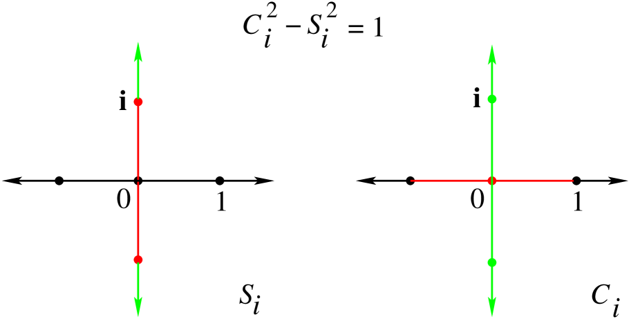
Figure 3: The three distinct color domains, black, red, and green, in the complex plane of the variable $S_{i}$ (left) and, under the relation $C_{i}^{2}-S_{i}^{2}=1$, the three corresponding domains of the variable $C_{i}$ (right).

Definition 2. For each bond $(S_{i},C_{i})$ we distinguish three possibilities, shown graphically in figure 3,

ii(i) “black” bond: $S_{i}$ an $C_{i}$ both real, which implies $|C_{i}|\geq 1$;

i(ii) “red” bond: $S_{i}$ imaginary and $C_{i}$ real, which implies $0<|S_{i}|\leq 1$ and $0\leq|C_{i}|<1$;

(iii) “green” bond: $S_{i}$ and $C_{i}$ both imaginary, which implies $|S_{i}|>1$ and $|C_{i}|>0$.

The color domains cover the union ${\mathbb{R}}\cup{\rm i}{\mathbb{R}}$ of the real and the imaginary axis. When $S_{i}$ is not in ${\mathbb{R}}\cup{\rm i}{\mathbb{R}}$ , then neither is $C_{i}$, and vice versa; such a coupling $(S_{i},C_{i})$ has no color assigned to it. For an initial lattice $\mathcal{T}(0)$ with arbitrary positive or negative couplings $K_{i}^{(0)}(\vec{r})$ all bonds are black and, to prove Theorem 1, we have to show that ST evolution does not generate couplings outside of ${\mathbb{R}}\cup{\rm i}{\mathbb{R}}$ .

3.2 Color transformation table

Table 1: Transformation (a) from triangle to star and (b) from star to triangle. “In” columns: list of possible ingoing color configurations, up to symmetry. “Out” columns: the corresponding outgoing color configurations, which depend on the sign of $F$.

Figure 4: (a) The three triangle sides (solid lines) with their three geometrically dual star legs (dashed). (b) For $i,j,k$ cyclic, side $i$ of the triangle and the pair $(j,k)$ of the star legs are said to be adjacent; similarly, leg $i$ of the star and the pair $(j,k)$ of the triangle sides are said to be adjacent.

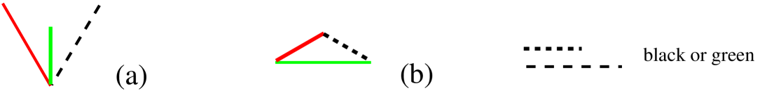
Figure 5: (a) Illustration of Property 4. (b) Illustration of Property 5.

We consider the ST transformation (2.4)-(2.5) from three given ingoing bonds $(S_{j},C_{j})$, each having one of the three colors black, red, or green, to three outgoing bonds $(S_{i}^{\,\prime},C_{i}^{\,\prime})$. We ask, given the colors of the ingoing bonds, what can be said about the colors of the outgoing bonds. The ingoing bond triplets that concern us, up to symmetry, are all listed in the “in” column of table 1a (for the steps triangle to star, $\mathcal{T}\mapsto\mathcal{H}$ ) and in the “in” column of table 1b (for the steps star to triangle, $\mathcal{H}\mapsto\mathcal{T}$ ). Notably absent from the “in” columns are those triangles or stars that have an odd number (one or three) of green bonds. This anticipates the result, still to be proven, that such in-triplets do not occur.

Equation (2.5) now implies that all ingoing triplets listed in table 1 lead to an $F$ that is real-valued. Equations (2.4)-(2.5) taken together then show that the three outgoing bonds have well-defined colors that are fully determined by those of the incoming bonds and  the sign of $F$. It is easy to verify that this leads to the entries shown in the “out” columns in table 1.

One may note that figures 1a and 1b are related by duality: by this we shall mean here the operation of replacing each bond with its geometrically dual bond (see figure 4a) while leaving the color unchanged.

3.3 Local properties

We still have to prove that table 1 actually covers all cases that may occur. To that end we first observe the following two properties of ST transformation (2.4)-(2.5).

Property 3a. Let an ingoing triplet consist of bonds $(S_{j},C_{j})$, with $j=1,2,3$, that all have one of the colors black, red, or green. Then $2+S_{1}^{2}+S_{2}^{2}+S_{3}^{2}$ is real and the variable $F$ moves off the real axis if and only if $C_{1}C_{2}C_{3}$ is pure imaginary. In that case the outgoing $(S_{i}^{\,\prime},C_{i}^{\,\prime})$ will not be in ${\mathbb{R}}\cup{\rm i}{\mathbb{R}}$ .

Property 3b. An ingoing triplet of bonds all having one of the colors black, red, or green will generate outgoing bonds not in ${\mathbb{R}}\cup{\rm i}{\mathbb{R}}$ if and only if an odd number (that is, one or three) of the ingoing bonds is green.

Proof of Properties 3a and 3b. It suffices to observe that the product $C_{1}C_{2}C_{3}$ is real for zero or two green bonds, and pure imaginary for one or three green bonds. $\square$

Three further properties will be needed. The first two of them involve the notion of adjacency, defined in figure 4b.

Property 4. Consider a star and a triangle associated with each other by ST transformation. A leg of the star is green if and only if exactly one of its two adjacent triangle sides is red.

Property 5. Consider a star and a triangle associated with each other by ST transformation. A side of the triangle is green if and only if exactly one of its two adjacent star legs is red.

Properties 4 and 5 are illustrated in figure 5a and 5b, respectively. These two properties are related by duality. Moreover, because of the “if and only if,” both properties may be applied in the step $\mathcal{T}\mapsto\mathcal{H}$ and in the step $\mathcal{H}\mapsto\mathcal{T}$. Their potential stems from the fact that only partial knowledge is needed about the colors of the three ingoing bonds (star legs or triangle sides) that participate in the transformation. We will invoke these properties repeatedly in sections 3.5, 5.1, and 5.2.

Proof of properties 4 and 5. One easily verifies these properties by examining all cases in figures 1a and 1b. $\square$

Property 6. If the number of ingoing green bonds in an ST  transformation is even (that is, zero or two), then the number of outgoing green bonds is also even.

Proof of Property 6. See table 1. $\square$

The properties listed so far are all local: they refer to the conversion of a local triplet of star legs into a local triplet of triangle sides, or vice versa, irrespective of their environment. In the next subsection we consider the interaction between neighboring triplets that arises as a consequence of the repartitionings that follow each iteration step.

3.4 Nonlocality

Each iteration of the ST transformation comprises two repartitionings of bonds, the first one (from up-stars to down-stars) after the step $\mathcal{T}\mapsto\mathcal{H}$, and the second one (from down-triangles to up-triangles) after the step $\mathcal{H}\mapsto\mathcal{T}$. The repartitionings rearrange the bonds into new triplets, and as a consequence the ST evolution becomes nonlocal. In order to efficiently discuss the implications of this we introduce two new definitions.

Definition 7a. A triangle in a triangular lattice is said to be even-green (EG) if it contains an even number (zero or two) of green sides. A triangular lattice is said to be even-green with respect to the up-triangles (EG_up) if all its up-triangles are EG; it is said to be even-green with respect to the down-triangles (EG_down) if all its down-triangles are EG. The lattice is said to be even-green (EG) if it is both EG_up and  EG_down.

Definition 7b. A star in a hexagonal lattice is said to be even-green (EG) if it contains an even number (zero or two) of green legs. A hexagonal lattice is said to be even-green with respect to the up-stars (EG_up) if all its up-stars are EG; it is said to be even-green with respect to the down-stars (EG_down) if all its down-stars are EG. The lattice is said to be even-green (EG) if it is both EG_up and  EG_down.

A lattice $\mathcal{T}(0)$ with real couplings $K_{i}^{(0)}(\vec{r})$ is obviously EG. Clearly if all lattices generated from $\mathcal{T}(0)$ in sequence (1.1) are EG, then, because of properties 3a and 3b, $F$ cannot move off the real axis and Theorem 1 is proved. We will therefore study in section 3.5 the transmission of the EG property under the action of the ST transformation.

We conclude this subsection with two corollaries that state nonlocal properties of EG lattices, and with two further definitions.

Corollary 8a. If a hexagonal lattice without boundaries is EG, then its green bonds constitute a collection of loops, and inversely. These loops are necessarily non-self-intersecting and not mutually intersecting.

Proof of Corollary 8a. Let there be an up-star two of whose bonds, say $\alpha$ and $\beta$, are green. Consider one of these bonds, say $\beta$. It is also part of a down-star, which because of the lattice being EG must contain a unique other green bond, say $\gamma$. But $\gamma$ is again also part of an up-star, etc. The sequence of bonds $\alpha$, $\beta$, $\gamma$, …, terminates only when it bites its own tail and then forms a loop. The inverse is immediate: if there were a star with one or three green legs, then these legs would not form loops. $\square$

Corollary 8b. If a triangular lattice without boundaries is EG, then the duals of its green bonds constitute a collection of loops on its dual hexagonal  lattice, and inversely. These loops are necessarily non-self-intersecting and not mutually intersecting.

Proof of Corollary 8b. Each bond of the dual lattice has the color of the corresponding primal bond. This dual lattice thus colored is hexagonal and, since under this duality EG triangles yield EG stars, it is EG. This reduces the proof to the case of Corollary 8a. $\square$

Definition 9a. A site of a triangular lattice is said to be even-red (ER) if it has an even number of red bonds (zero, two, four, or six) connected to it. A triangular lattice is said to be ER if all its sites are ER.

Definition 9b. An elementary six-legged loop on a hexagonal lattice is said to be even-red (ER) if it contains an even number (zero, two, four, or six) of red legs. A hexagonal lattice is said to be ER if all its elementary loops are ER.

We are now prepared for the proof of the main theorem.

3.5 Main theorem

Figure 6: Illustration of Step 1 in the proof of Theorem 10. (a) An offending down-star on lattice $\mathcal{H}(n)$, having an odd number of green legs. (b) Thin dashed lines indicate the three up-triangles on lattice $\mathcal{T}(n)$ that generated the three star legs. (c) One subset of several possible color configurations of the triangle sides that would lead to the offending down-star; these color configurations all violate the ER property of $\mathcal{T}(n)$, thus showing that the down-star in (a) cannot occur. Note that the only triangle sides whose colors matter are the six that join the star center. Figures (d), (e), and (f) are analogous to (a), (b), and (c), but for a different offending down-star.

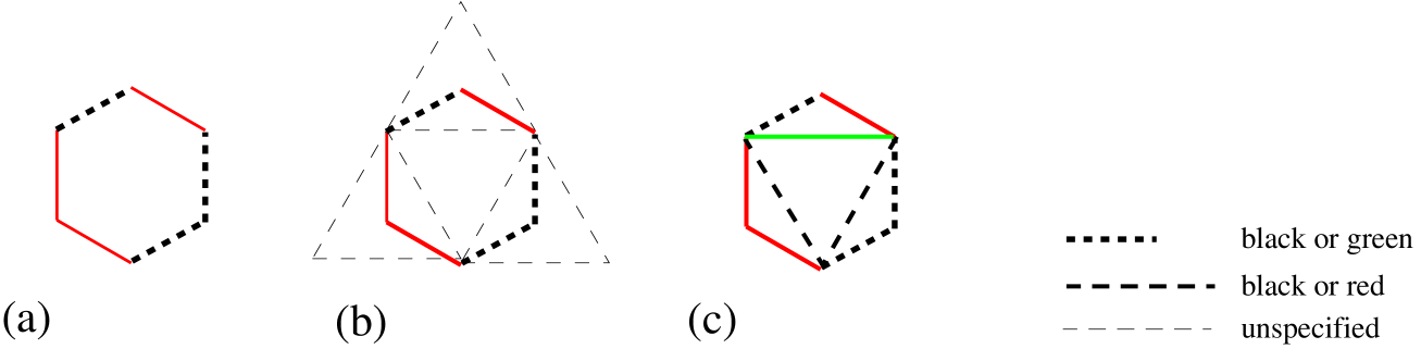
Figure 7: Illustration of Step 1 in the proof of Theorem 10. (a) An offending hexagonal loop on lattice $\mathcal{H}(n)$, having an odd number of red legs. (b) Thin dashed lines indicate the three up-triangles on lattice $\mathcal{T}(n)$ that generated the six legs of the loop. (c) One subset of several possible color configurations of the three sides of the central down-triangle that would lead to the offending hexagonal loop; these configurations all violate the EG_down property, thus showing that the hexagonal loop in (a) cannot occur. Note that there are only three triangle sides whose colors matter.

Theorem 10. Let an initial lattice $\mathcal{T}(0)$ be EG and ER. Then under the ST  evolution (1.1) all subsequent lattices $\mathcal{H}(n)$ for $n=0,1,2,\ldots$ and  $\mathcal{T}(n)$  for $n=1,2,\ldots$ are EG and ER.

Proof of Theorem 10. The proof proceeds by induction and amounts to checking all in- and outgoing color combinations that may occur. Step 1 transfers the properties of being EG and ER from $\mathcal{T}(n)$ to $\mathcal{H}(n)$, and Step 2 transfers them from $\mathcal{H}(n)$ to $\mathcal{T}(n+1)$.

Step 1: $\mathcal{T}\mapsto\mathcal{H}$. — Let $\mathcal{T}(n)$ be both EG and ER and suppose that $\mathcal{H}(n)$ is not. We will show that this leads to a contradiction.

Suppose first that $\mathcal{H}(n)$ is not EG. Since the EG_up property of $\mathcal{H}(n)$ follows from the EG_up property of $\mathcal{T}(n)$  we must then have that $\mathcal{H}(n)$ is not EG_down. This means there is an “offending” down-star of the type shown in figure 6a (possibly up to a rotation) or in 6d, having either one or three green bonds. The dashed black bonds in figure 6a stand for bonds that may be either red or black. We now trace these two configurations one step back. The three legs were generated by three different up-triangles of the lattice $\mathcal{T}(n)$, shown by thin dashed lines in figures 6b and 6e. Each of the three star legs has two adjacent triangle sides, and these six sides come together at the center of the down-star. Now by Property 4, a leg can be green if and only if among the two adjacent sides of its generating triangle there is an odd number (necessarily one) of red sides. The number of red triangle sides joining in the star center is therefore: in figure 6c, the sum of an odd integer (one) and two even integers (equal to zero or to two) and in figure 6f, the sum of three odd integers (each equal to one). Hence this number is odd, which contradicts the premise that $\mathcal{T}(n)$ is ER. It follows that $\mathcal{H}(n)$ is EG.

Suppose, secondly, that $\mathcal{H}(n)$ is not ER. This means there is an offending elementary six-legged loop that has an odd number of red legs. An example of such a loop is shown in figure 7a. These legs were generated pairwise in three independent up-triangles of $\mathcal{T}(n)$, shown by thin dashed lines in figure 7b. They together enclose a central down-triangle each of whose sides is adjacent to two consecutive legs of the loop. Now by Property 5, such a leg pair has an odd number (hence exactly one) of red legs if and only if the adjacent side of the generating triangle is green. Therefore, an odd number of red legs in the loop implies that the central down-triangle has an odd number of green sides. This contradicts the premise that $\mathcal{T}(n)$ is EG. It follows that $\mathcal{H}(n)$ is ER.

Hence $\mathcal{H}(n)$ is both EG and ER.

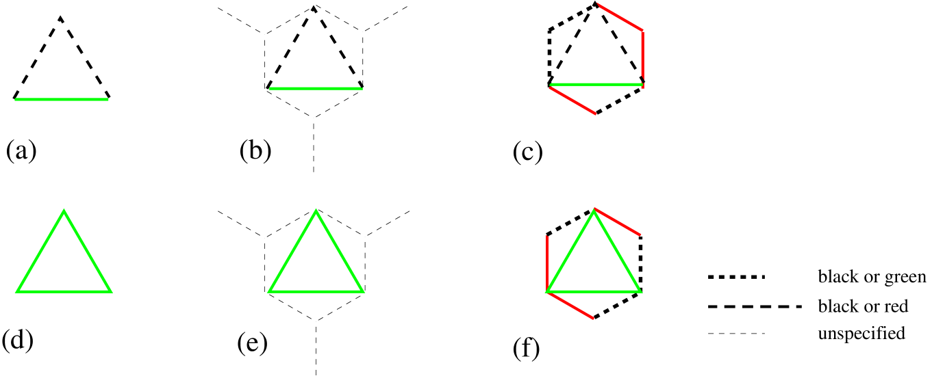
Figure 8: Illustration of Step 2 in the proof of Theorem 10. (a) An offending up-triangle on lattice $\mathcal{T}(n+1)$, having an odd number of green legs. (b) Thin dashed lines indicate the three down-stars on lattice $\mathcal{H}(n)$ that generated the three triangle sides. (c) One subset of several possible color configurations of the star legs that would lead to the offending up-triangle; these configurations all violate the ER property of $\mathcal{H}(n)$, thus showing that the up-triangle in (a) cannot occur. Note that the only six star legs whose colors matter are those that are part of the hexagonal loop around the triangle in (a). Figures (d), (e), and (f) are analogous to (a), (b), and (c), but for a different offending up-triangle.

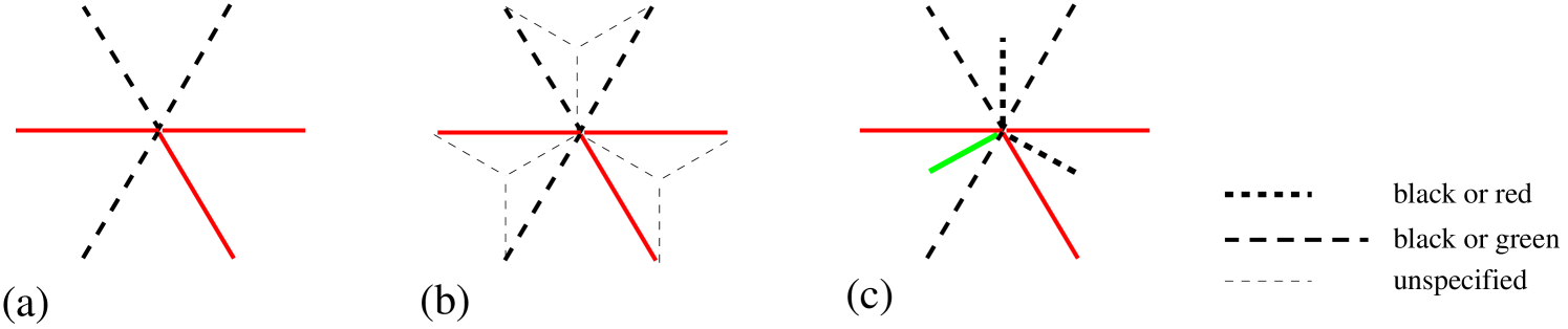
Figure 9: Illustration of Step 2 in the proof of Theorem 10. (a) An offending site on $\mathcal{T}(n+1)$, joined by an odd number of red triangle sides. (b) Thin dashed lines indicate the three down-stars on lattice $\mathcal{H}(n)$ that generated the six triangle sides joining the offending site. (c) One subset of several possible color configurations of the three legs of the central down-star that would lead to the offending site; these configurations all violate the EG_up property of $\mathcal{H}(n)$, thus showing that the site in (a), where three triangle sides join, cannot occur. Note that the only three star legs whose colors play a role are those shown in (c).

Step 2: $\mathcal{H}\mapsto\mathcal{T}$. — Let $\mathcal{H}(n)$ be both EG and ER and suppose that $\mathcal{T}(n+1)$ is not. We will show that this leads to a contradiction.

This step is related to Step 1 by symmetry under duality. We nevertheless repeat the reasoning because it will be of help in the next section in discussing a system with boundaries, for which the same duality is absent. Local color configurations relevant to this step are shown in figure 8.

Suppose first that $\mathcal{T}(n+1)$ is not EG. Since its EG_down property follows from the EG_down property of $\mathcal{H}(n)$, we must then have that $\mathcal{T}(n+1)$ is not EG_up. This means there must be an offending up-triangle which, possibly up to a rotation, is of the type shown in figure 8a or 8d, having either one or three green sides. Again, the dashed black lines in 8a stand for bonds that may be either red or black. The three triangle sides were generated by three different down-stars of the lattice $\mathcal{H}(n)$, shown in figures 8b and 8e as thin dashed lines. Each of the three triangle sides has two adjacent legs, and these six legs constitute an elementary loop of $\mathcal{H}(n)$. Now when Property 5 is applied to the three down-stars, we find that this elementary loop contains an odd number of red legs as shown in 8c and 8f. This contradicts the premise that $\mathcal{H}(n)$ is ER. Hence $\mathcal{T}(n+1)$ is ER.

Suppose, secondly, that $\mathcal{T}(n+1)$ is not ER. Then it must have an offending site where an odd number of red triangle sides come together. An example of such a is shown in figure 9a. The six sides were generated pairwise by three distinct down-stars of $\mathcal{H}(n)$, shown by thin dashed lines in figure 9b. Each down-star contributes two sides, of which, by Property 4, exactly one is red if and only if the adjacent star leg is green. Since there is an odd number of red sides, there must also be an odd number of green star legs joining at the same site. This contradicts the premise that $\mathcal{H}(n)$ is EG. Hence $\mathcal{T}(n+1)$ is ER.

Upon combining the results of Steps 1 and 2 we conclude that $\mathcal{T}(n+1)$ is both EG and ER, which proves Theorem 10. $\square$

We now return to Theorem 1.

Proof of Theorem 1. A triangular lattice that has only positive or negative couplings has only black bonds and is therefore trivially EG and ER. Hence Theorem 1 is the special case of Theorem 10 that applies to physical systems. $\square$

3.6 Numerical evaluation

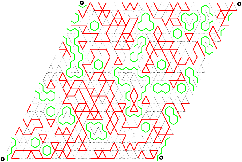
Figure 10: Snapshot of the bond coloring of lattice ${\mathcal{T}}(100)$. The lattice is periodic in two directions, the four encircled sites being identical. The figure was obtained from an initial lattice $\mathcal{T}(0)$ with random coupling strengths $S_{i}^{(0)}(\vec{r})=1/\sinh 2K_{i}^{(0)}(\vec{r})$ drawn independently for each bond from a uniform distribution on $[-0.5,0.5]$. For greater clarity, instead of showing the green bonds of ${\mathcal{T}}(100)$ themselves, the figure shows their duals. See text.

We performed the ST evolution numerically for a triangular lattice of $20\times 20$ sites with periodic boundary conditions. The initial lattice ${\mathcal{T}}(0)$ has coupling strengths $K_{i}^{(0)}(\vec{r})$ drawn randomly and independently from a distribution symmetric about zero, i.e., the system is a standard 2D symmetric Ising spin glass. Although initially all bonds are black, the frustration of a fraction of the elementary triangles leads to the appearance of red and green bonds after the first iteration. Figure 10 shows the bond colors of lattice ${\mathcal{T}}(100)$, obtained after $100$ iterations. For greater clarity it does not show the green triangle sides themselves, but rather their duals as defined by figure 4a, which are star legs. The green star legs are seen to form loops in agreement with Corollary 8b and with the lattice being EG. Moreover, each lattice site is joined by an even number, possibly zero, of red bonds, in agreement with Definition 9a and with the lattice being ER.

We have briefly considered the numerical errors incurred under ST transformation. We applied to an initial lattice ${\mathcal{T}}(0)$ of size $20\times 20$ first $n$ forward iterations so as to obtain ${\mathcal{T}}(n)$, and then $n$ backward iterations leading to a final lattice ${\mathcal{T}}^{\,\prime}(0)$; in the absence of numerical errors we would have ${\mathcal{T}}^{\,\prime}(0)={\mathcal{T}}(0)$. We took as our criterion an average discrepancy of one percent between corresponding bond strengths of the initial and the final lattice. For a symmetric distribution (whether dichotomic, block, or Gaussian) of the initial coupling strengths $S_{i}=S_{i}^{(0)}(\vec{r})$ we found that under this criterion, and using standard double precision, we could safely iterate up to but not beyond $n\approx 200$ for $\langle S_{i}\rangle^{1/2}=\pm 2.0$ (high temperature) and up to but not beyond $n\approx 100$ for $\langle S_{i}\rangle^{1/2}=\pm 0.2$ (low temperature). This accuracy for the symmetric spin glass appears to be low compared to what one obtains in the ferromagnetic regime (all couplings random but positive); in that regime we found that, depending on the exact parameters, $n$ may easily take values as high as $10^{4}$ or $10^{5}$.

There is a physical explanation for the strongly deteriorated accuracy in the case of a symmetric spin glass, namely the cancellations that occur between energy and entropy in the calculation of the system free energy. In the spin glass phase, i.e. below the critical spin glass temperature $T_{g}$, such cancellations were explained by Fisher and Huse [32, 33] in terms of their “droplet model.” Thill and Hilhorst [34] showed the relevance of similar cancellations also in the temperature region closely above  the critical temperature, which for the 2D spin glass has the value $T_{g}=0$. In the limit $T\to T_{g}$ these cancellations lead to the 2D spin glass having two nontrivial exponents, the temperature exponent $y$ and the chaos exponent $\zeta$. One may speculate that there is a way, still to be devised, to calculate these exponents with the aid of the ST transformation.

4 ST evolution in the presence of boundaries

The preceding sections apply to a lattice that does not have boundaries, as happens when it is infinite or when suitable boundary conditions (e.g. periodic ones) are imposed. However, some of the most interesting applications of the ST transformation have involved lattices with boundaries, and such systems must be considered separately. When a triangular (a hexagonal) lattice with a boundary is partitioned into up-triangles or down-triangles (into up-stars or down-stars), there remain at the boundary triangles (stars) that are incomplete, i.e., that do not have the full set of three bonds. We will show how the ST transformation applies to such incomplete triangles and stars, and will conclude that modified versions of Theorem 1 remain valid.

Figure 11: (a) Thin solid lines: lattice $\mathcal{T}(n)$, filling a horizontal slab of vertical width $L=L_{+}-L_{-}$. Horizontally it may be infinite or periodic. Thick dashed lines: lattice $\mathcal{H}(n)$ obtained from $\mathcal{T}(n)$ by ST transformation. (b) The same lattice $\mathcal{H}(n)$ and, in thick solid lines, lattice $\mathcal{T}(n+1)$ obtained from it by ST transformation.

4.1 Advancing and receding boundaries

The simplest example of a lattice with boundaries is the triangular lattice $\mathcal{T}(n)$ shown in figure 11a. It fills a slab of finite width $L=L_{+}-L_{-}$ in the vertical direction and may be either infinite or periodic in the horizontal direction. In Step 1 of the $(n+1)$th ST iteration it gets transformed into the hexagonal lattice $\mathcal{H}(n)$ shown in thick dashed lines in figure 11a and reproduced in 11b. In Step 2 of the same iteration it gets transformed into the triangular lattice $\mathcal{T}(n+1)$ indicated by thick solid lines in figure 11b. Lattice $\mathcal{T}(n+1)$ is a slab that is geometrically identical to $\mathcal{T}(n)$ but its bond strengths have changed and it has moved in the vertical direction by a distance equal to one third of the vertical separation between two successive rows. The ST transformation in such slabs (but restricted to ferromagnetic interaction) was studied by Burkhardt and Guim [18, 20] and by Lajkó and Iglói [21]. This transformation involves two special types of ingoing bond configurations:

i(i) In Step 1 the bonds in the top row (row $L_{+}$) of the lattice are isolated triangle sides. Decorating such a single-sided “triangle” amounts to inserting a new spin variable between the two spins joined by that side, which replaces the single triangle side by a pair of star legs.

(ii) In Step 2 each spin in the bottom row (row $L_{-}$) is connected to only two star legs; it is the center of an incomplete down-star. Decimating this spin produces a single triangle side.

Clearly the two borders are not equivalent: the upper border advances (moves into previously empty space), and the lower border recedes (withdraws from previously occupied space). Obviously by setting $L_{+}=\infty$ (or $L_{-}=\infty$) we obtain a half-infinite system with only a receding (or only an advancing) boundary.

Below we will first establish the special ST transformation formulas applicable at the boundaries and then study the corresponding evolution of the bond colors.

4.2 Boundary star-triangle transformation

At the boundaries the symmetry argument that motivated definitions (2.1)-(2.2) is of very limited use. We will therefore in this section, in deviation from those definitions, reserve the notation $S_{i}$ and $C_{i}$ for the bonds of a two-legged star, whence

$$S_{i}=\sinh 2p_{i}\,,\qquad C_{i}=\cosh 2p_{i}\,,\qquad i=2,3,$$ (4.1)

whereas for an isolated triangle side we adopt the notation

$$X_{1}=1/\sinh 2K_{1}\,,\qquad Y_{1}=\coth 2K_{1}\,.$$ (4.2)

Obviously

$$C_{i}^{2}-S_{i}^{2}=1,\qquad Y_{1}^{2}-X_{1}^{2}=1.$$ (4.3)

We will consider separately the incomplete decimation (star-to-triangle, $\mathcal{H}\mapsto\mathcal{T}$) and the incomplete decoration (triangle-to-star, $\mathcal{T}\mapsto\mathcal{H}$).

Table 2: Special cases at boundaries. Transformation (a) from a single triangle side at an advancing boundary into an incomplete two-legged star and (b) from an incomplete two-legged star at a receding boundary into a single triangle side.

4.2.1 From a two-legged star to a single triangle side

At a receding boundary we have to deal with incomplete two-legged stars. Decimating the central spin of such a star generates a single triangle side. Its strength $K_{1}$ follows from the general case [equations (2.1) and (2.4)] when we set $p_{1}=0$ and hence $S_{1}=0$ and $C_{1}=1$. We find, now using the notation of equation (4.2), that

$$X_{1}=\frac{C_{2}+C_{3}}{S_{2}S_{3}}\,,\qquad Y_{1}=\frac{1+C_{2}C_{3}}{S_{2}S_{3}}\,.$$ (4.4)

With the aid of (4.4) and Definition 2 one easily finds the color transformation rules listed in table 2b. The color of the triangle side generated follows deterministically by the colors of the two ingoing star legs. Absent from the “in” column are leg pairs of which exactly one leg is green. Such an ingoing pair would lead to an outgoing bond not in ${\mathbb{R}}\cup{\rm i}{\mathbb{R}}$ , and below we will show that such a pair cannot occur.

4.2.2 From a single triangle side to a two-legged star

At an advancing boundary we have to deal with single triangle sides. Decorating such a side by a central spin generates a two-legged star. This transformation may at first sight appear as the mere inverse of equation (4.4); however, since (4.4) maps the two bonds $(S_{2},C_{2})$ and $(S_{3},C_{3})$ onto the single bond $(X_{1},Y_{1})$, the inverse is not unique. This point requires a more detailed discussion, which becomes easier when with the aid of some simple hyperbolic trigonometry we write (4.4) in the alternative form

$$\tanh K_{1}=\tanh p_{2}\,\tanh p_{3}\,,$$ (4.5)

a relation well-known in 1D decimation. For given $K_{1}$ this equation admits for the pair $(p_{2},p_{3})$ a two-dimensional continuum of solutions that may be parametrized as

$$\tanh p_{2}=z(\tanh K_{1})^{1/2},\qquad\tanh p_{3}=z^{-1}(\tanh K_{1})^{1/2},$$ (4.6)

where $z$ is any nonzero complex number and we may arbitrarily choose either of the square roots of $\tanh K_{1}$. For general $z$ this would put $S_{2},C_{2},S_{3}$, and $C_{3}$ outside of ${\mathbb{R}}\cup{\rm i}{\mathbb{R}}$ . We will not explore here the consequences of such a general choice of $z$, but simply impose  that the $S_{i}$ and $C_{i}$ remain confined to ${\mathbb{R}}\cup{\rm i}{\mathbb{R}}$ . This still leaves, for given $K_{1}$, a one-dimensional continuum of possible solutions $(p_{2},p_{3})$ to (4.5), out of which we will select a convenient one. We have to distinguish two cases, depending on the color of the ingoing bond $K_{1}$.

$K_{1}$ is black or red. — Let the triangle side $K_{1}$ be given. We select a unique solution by imposing the additional restriction $p_{2}=p_{3}$. This means setting $z=1$ in equation (4.6) and leads to

$$\tanh p_{2}=\tanh p_{3}=(\tanh K_{1})^{1/2}.$$ (4.7)

We may now revert to the variables of equations (4.1)-(4.2). With the aid of the relation $\tanh K_{1}=Y_{1}-X_{1}$ and some further algebra we find that (4.7) leads to

$$S_{2}=S_{3}=\frac{\sqrt{2(Y_{1}-X_{1})}}{1-Y_{1}+X_{1}}\,,\qquad C_{2}=C_{3}=\frac{Y_{1}+1}{X_{1}}\,,$$ (4.8)

which constitutes a solution to (4.5), and in which the sign of the square root may be chosen arbitrarily. With the aid of (4.8) one easily finds the transformation rules for the colors listed in table 2a. The two cases with black or red $K_{1}$ correspond to $Y_{1}$ being real with $Y_{1}^{2}>1$ or $0<Y_{1}^{2}<1$, respectively. Moreover, for black $K_{1}$ the two subcases $Y_{1}>0$ and $Y_{1}<0$ have to be distinguished.

$K_{1}$ is green. — When the ingoing triangle side $K_{1}$ is green, then $Y_{1}$ and $X_{1}$ are pure imaginary. If we were again to set $z=1$, whence as before solution (4.8), the couplings $S_{i}$ and $C_{i}$ $(i=2,3)$ would be outside ${\mathbb{R}}\cup{\rm i}{\mathbb{R}}$ , against our wish. We therefore look for a different solution.

We note that in this case $K_{1}$ is pure imaginary, too, and we therefore set $K_{1}={\rm i}L_{1}$, the relevant values being $-\tfrac{\pi}{4}<L_{1}<\tfrac{\pi}{4}$. Preparing now for the symmetry between $p_{2}$ and $p_{3}$ to be broken we let $p_{3}={\rm i}q_{3}$ so that equation (4.5) becomes

$$\tan L_{1}=\tanh p_{2}\tan q_{3}\,.$$ (4.9)

We select the solution

$$\tanh p_{2}=\tan q_{3}=(\tan L_{1})^{1/2},$$ (4.10)

which amounts to setting $z=\mbox{e}^{{-\rm i}\pi/4}$ in (4.6) and is such that $\tanh p_{2}$ and $\tan q_{3}$ are either both real or both imaginary. When reverting to the variables of equations (4.1)-(4.2) and with the aid of the relation $\tanh K=-{\rm i}(Y_{1}-X_{1})$ we find that (4.10) leads to

$$S_{2}=\frac{2\sqrt{-{\rm i}(Y_{1}-X_{1})}}{1+{\rm i}(Y_{1}-X_{1})}\,,\qquad C_{2}=\frac{1-{\rm i}(Y_{1}-X_{1})}{1+{\rm i}(Y_{1}-X_{1})}\,,$$ (4.11a)

$$S_{3}=\frac{2{\rm i}\sqrt{-{\rm i}(Y_{1}-X_{1})}}{1-{\rm i}(Y_{1}-X_{1})}\,,\qquad C_{3}=\frac{1+{\rm i}(Y_{1}-X_{1})}{1-{\rm i}(Y_{1}-X_{1})}\,,$$ (4.11b)

which constitutes a solution to (4.5). Since ${\rm i}(Y_{1}-X_{1})$ is real, so are $C_{2}$ and $C_{3}$, which moreover are seen to satisfy the relation $C_{2}C_{3}=1$. For ${\rm i}(Y_{1}-X_{1})<0$ we have that $S_{2}$ is real and $S_{3}$ imaginary, and for ${\rm i}(Y_{1}-X_{1})>0$ the opposite is the case. This means that among $p_{2}$ and $p_{3}$ one is black and the other one red. Hence equations (4.11a) and (4.11b) allow us to establish the last line in table 2a.

We end this subsection with a remark about the symmetry between $p_{2}$ and $p_{3}$. Setting $z=\mbox{e}^{{-\rm i}\pi/4}$ in (4.6) leads to solution (4.10), which breaks this symmetry. Setting alternatively $z=\mbox{e}^{+{\rm i}\pi/4}$ breaks the symmetry the other way around and exchanges in equations (4.11) the expressions for $(S_{2},C_{2})$ with those for $(S_{3},C_{3})$, that is, it interchanges the red and the black star leg. There is no reason why one choice would be preferable over the other. In the next subsection we address the consequences of this remaining freedom.

4.3 Irreversibility and protocols

The choice between the two symmetry-related solutions of the preceding subsection may be made independently for each triangle side in the advancing boundary, and independently at Step 1 of each iteration. Clearly in order to fully define ST evolution of a lattice with an advancing boundary, we have to specify a protocol. We may, for example, assign probabilities $\eta$ and $1-\eta$, with $0\leq\eta\leq 1$, to the two possibilities, and will refer to this procedure as the “random protocol.” In the numerical example of section 5.5 below we have chosen the “uniform random protocol” $\eta=1/2$. Protocols based on values other than $z=\mbox{e}^{\pm{\rm i}\pi/4}$ are easily imagined and some may be better than others for specific applications; we have not pursued that line of investigation.

When a lattice $\mathcal{T}(0)$ with an advancing boundary is submitted to $n$ iterations of the ST evolution under any protocol and yields $\mathcal{T}(n)$, then if we invert the evolution the advancing boundary becomes a receding one, the effect of the protocol is wiped out again, and the initial state $\mathcal{T}(0)$ is reached.

At a receding boundary the ST evolution is fully deterministic. However, it is irreversible: its inverse, under which the boundary becomes advancing, is not uniquely defined and the initial state $\mathcal{T}(0)$ cannot be reconstructed from the knowledge of $\mathcal{T}(n)$.

5 Bond color evolution at boundaries

The preceding discussion makes clear that for a system with boundaries the formulation of Theorem 1 needs to be modified. We present and prove these modified theorems below. We do not attempt at full generality but consider only semi-infinite systems with a single straight boundary, as obtained from figure 11 by setting either $L_{+}=\infty$ or $L_{-}=\infty$.

Theorem 11. Let a triangular lattice $\mathcal{T}(0)$ with a receding boundary have arbitrary positive or negative initial couplings $K_{i}^{(0)}(\vec{r})$. Then under star-triangle evolution, with (2.4)-(2.5) replaced at the boundary by (4.4), the couplings $S_{i}^{(n)}(\vec{r})$ and $C_{i}^{(n)}(\vec{r})$ of the lattices $\mathcal{T}(n)$ and $\mathcal{H}(n)$, where $n=0,1,2,\ldots$, remain confined to the union of the real and imaginary axis.

Theorem 12. Let a triangular lattice $\mathcal{T}(0)$ with an advancing boundary have arbitrary positive or negative initial couplings $K_{i}^{(0)}(\vec{r})$. Then under star-triangle evolution, with (2.4)-(2.5) replaced at the boundary by (4.8) or by (4.11) and for the random protocol discussed in section 4.3, the couplings $S_{i}^{(n)}(\vec{r})$ and $C_{i}^{(n)}(\vec{r})$ of the lattices $\mathcal{T}(n)$ and $\mathcal{H}(n)$, where $n=0,1,2,\ldots$, remain confined to the union of the real and imaginary axis.

To prepare for the proof of these two theorems, we need to slightly extend Definitions 7a and 7b of the EG property in order for these to include the case of a lattice with boundaries.

Definition 13a. A triangular lattice with a receding and/or advancing boundary is said to be EG_up (EG_down) if all its complete up-triangles (complete down-triangles) are EG_up (EG_down). The lattice is said to be EG if it is both EG_up and EG_down.

Definition 13b. A two-legged star is said to be EG if it contains an even number (zero or two) of green legs. A hexagonal lattice with a receding and/or advancing boundary is said to be EG_up (EG_down) if all its complete and incomplete up-stars (down-stars) are EG. The lattice is said to be EG if it is both EG_up and EG_down.

It may be noted that Definition 13a imposes no condition on incomplete triangles, but that Definition 13b does include a condition on incomplete stars. Definitions 9a and 9b of the ER property remain unchanged. Concerning Definition 9a we note that at a boundary site at most four triangle sides may join; and concerning Definition 9b we note that all elementary loops are six-legged.

In view of the preceding observations and extended definitions Theorems 11 and 12 will be proved if we can show that in each of the steps $\mathcal{T}(n)$$\,\mapsto$$\mathcal{H}(n)$ and $\mathcal{H}(n)$$\,\mapsto$$\mathcal{T}(n+1)$, where $n=0,1,2,\ldots$, the property of the lattice being EG is transmitted from the ingoing to the outgoing lattice. As before, we will show that in fact ER and EG, now obeying Definitions 9 and 13, respectively, are transmitted together. Things amount, therefore, to proving the induction step: if $\mathcal{T}(n)$ is EG and ER, then so is $\mathcal{H}(n)$, and if $\mathcal{H}(n)$ is EG and ER, then so is $\mathcal{T}(n+1)$. We prove this for the receding boundary (Theorem 11) in section 5.1 and for the advancing boundary (Theorem 12) in section 5.2. The reasoning will be along the same lines as that in section 3.5, with many color combinations to be checked separately. We will illustrate these by the diagrammatic representation of figure 12, which serves the same purpose as figures 6 through 9, but is more compact.

Figure 12: In the proofs of Theorems 11 and 12 we consider figures (a)-(d) and (e)-(h), respectively. The top row of figures represent the step $\mathcal{T}(n)$ $\mapsto$ $\mathcal{H}(n)$ and the bottom row the step $\mathcal{H}(n)$ $\mapsto$ $\mathcal{T}(n+1)$. In each figure the solid lines represent the putative offending configuration; heaviness of a solid line, and of the dot in figure (g), indicates that it is located on the boundary. The dashed lines represent the stars or triangles, complete or incomplete, that in the preceding step gave rise to the offending configuration. The offending configurations are the following: (a) an incomplete two-legged down-star having exactly one green leg; (b) a hexagonal loop having an odd number of red legs; (c) an up-triangle having an odd number of green sides; (d) a site where four triangle sides join, out of which an odd number is red; (e) a down-star having exactly one green leg; (f) a hexagonal loop having an odd number of red legs; (g) an up-triangle having an odd number of green sides; (h) a site where four triangle sides join, out of which an odd number is red. In each of these eight figures several different colorings are possible.

5.1 Receding boundary

We consider the semi-infinite lattice obtained by letting $L_{+}\to\infty$ in figure 11. The boundary at the bottom of this lattice is receding.

Proof of Theorem 11.

Step 1: $\mathcal{T}\mapsto\mathcal{H}$. — Let $\mathcal{T}(n)$ be both EG and ER and suppose that $\mathcal{H}(n)$ is not. We will show that this leads to a contradiction.

Suppose first that $\mathcal{H}(n)$ is not EG. Since in this step all ingoing up-triangles are complete, $\mathcal{H}(n)$ is necessarily EG_up, and so we must then have that $\mathcal{H}(n)$ is not EG_down. This means $\mathcal{H}(n)$ has an offending down-star with an odd number of green bonds. If that down-star is in the bulk we have seen in section 3.5 that this leads to a contradiction, as was illustrated by figure 6. Now let the offending down-star be an incomplete two-legged star on the bottom boundary of $\mathcal{H}(n)$. The star legs are shown in figure 12a as solid lines, their thickness indicating that they are part of the boundary. The offense of this incomplete star is to have exactly one green leg (it could be either of the two shown and the figure does not distinguish between the two possibilities). Now we trace back the origin of these two legs: in the preceding step they were generated independently by two distinct up-triangles, shown in the same figure as thin dashed lines. Upon applying in both triangles Property 4 (figure 5a, rotated by $\pm 2\pi/3$ and if necessary first mirrored with respect to its central axis) we see that out of the four triangle sides joining at the center site, the number of red ones is either one or three. This contradicts the premise of $\mathcal{T}(n)$ being ER. It follows that $\mathcal{H}(n)$ is EG.

Suppose, secondly, that $\mathcal{H}(n)$ is not ER. Then there is an elementary six-legged loop containing an odd number of red legs. We have to check the case, shown in figure 12b, where this loop contains one site of the bottom boundary. It is easily seen that this leads to a contradiction in the same way as in the bulk, where it was illustrated by figure 7. It follows that $\mathcal{H}(n)$ is ER.

Hence $\mathcal{H}(n)$ is EG and ER.

Step 2: $\mathcal{H}\mapsto\mathcal{T}$. — Let $\mathcal{H}(n)$ be both EG and ER and suppose that $\mathcal{T}(n+1)$ is not. We will show that this leads to a contradiction.

Suppose first that $\mathcal{T}(n+1)$ is not EG. Since this lattice was constructed by ST transformations in down-triangles, it is necessarily EG_down. So we must then have that $\mathcal{T}(n+1)$ is not EG_up. This means that $\mathcal{T}(n+1)$ has an offending up-triangle having either a single or three green sides, as was illustrated in figure 8 for the bulk. Suppose now that the offending up-triangle has one side on the bottom boundary of $\mathcal{T}(n+1)$, as shown in figure 12c. This side was generated by an incomplete down-triangle, shown by thin dashed lines in the same figure, and this ST transformation satisfies Property 5: it contributes a green triangle side if and only if exactly one of its two legs is red. Therefore, just as in the bulk, we conclude that the hexagonal loop in $\mathcal{H}(n)$ that surrounds the offending up-triangle has an odd number of red legs, which contradicts the premise of $\mathcal{H}(n)$ being ER. It follows that $\mathcal{T}(n+1)$ is EG.

Suppose, secondly, that $\mathcal{T}(n+1)$ is not ER. Then there is an offending site where an odd number of red triangle sides come together. If that site is in the bulk, we have seen that this leads to a contradiction, as was illustrated by figure 9. Now let that site be on the boundary, as shown in figure 12d. It is then connected to four triangle sides out of which either one or three are red. The two horizontal ones of these sides were generated by incomplete down-stars of $\mathcal{H}(n)$, and the other two by a single complete down-star of $\mathcal{H}(n)$. By using again Property 5 we find that the up-star of $\mathcal{H}(n)$ centered at the offending site must have had an odd number of green legs, which contradicts the premise of $\mathcal{H}(n)$ being EG. It follows that $\mathcal{T}(n+1)$ is ER.

Hence $\mathcal{T}(n+1)$ is EG and ER. This proves Theorem 11. $\square$

5.2 Advancing boundary

We consider the semi-infinite lattice obtained by letting $L_{-}\to\infty$ in figure 11. The boundary at the top of this lattice is advancing.

Proof of Theorem 12.

Step 1: $\mathcal{T}\mapsto\mathcal{H}$. – Let $\mathcal{T}(n)$ be both EG and ER and suppose that $\mathcal{H}(n)$ is not. We will show that this leads to a contradiction.

Suppose first that $\mathcal{H}(n)$ is not EG. Those ingoing up-triangles of $\mathcal{T}(n)$ that are complete all lead to up-stars that are EG_up. The up-stars of $\mathcal{H}(n)$ located in the bulk were all generated by complete up-triangles of $\mathcal{T}(n)$ and therefore are EG_up. The top boundary of $\mathcal{H}(n)$ is a zigzagging sequence of star legs; each pair of legs was generated by a single triangle side according to the rules symbolized in table 2a, which show that a pair so generated contains either zero or two green legs. Each such pair constitutes an incomplete two-legged up-star, and therefore by Definition 13b these incomplete up-stars are also EG_up. Therefore, by the same definition, lattice $\mathcal{H}(n)$ is EG_up. Since we supposed that $\mathcal{H}(n)$ is not EG, it must then fail to be EG_down. This means $\mathcal{H}(n)$ has an offending down-star with an odd number of green bonds. If that down-star is in the bulk we have seen that this leads to a contradiction, as was illustrated by figure 6. Now let the offending down-star have its two upper legs on the top boundary of $\mathcal{H}(n)$, as shown in figure 12e. These upper legs were generated by two isolated triangle sides, both shown as thin dashed horizontal lines; whereas the vertical leg was generated by a full triangle, also shown thin dashed. We may apply Property 4 (see figure 5a) to the vertical leg and conclude that if and only if it is green, then it will contribute exactly one red triangle side joining the central site. And for each of the two upper legs, we may use table 2a to conclude that if it is green, then it must have resulted from a triangular side that was red. It follows that in $\mathcal{T}(n)$ the down-star center, viewed as a site of $\mathcal{T}(n)$, was joined by an odd number of red triangle sides. This contradicts the premise of $\mathcal{T}(n)$ being ER. It follows that $\mathcal{H}(n)$ is EG.

Suppose, secondly, that $\mathcal{H}(n)$ is not ER. This means $\mathcal{H}(n)$ has an offending elementary six-legged loop containing an odd number of red legs. We have seen that if the offending loop is in the bulk, this leads to a contradiction as illustrated by figure 7. If the loop is in the top row of loops, as shown in figure 12f, then the top one of these triangles is single-sided; nevertheless, together with the two complete up-triangles it encloses a down-triangle. But Property 5 governs in the same way the relation between the red star legs in the loop and the green triangle sides in the down-triangle. We find that its number of green sides must be odd, which contradicts the premise that $\mathcal{T}(n)$ is EG. This leads to a contradiction in the same way as in the bulk. It follows that $\mathcal{H}(n)$ is ER.

Hence $\mathcal{H}(n)$ is EG and ER.

Step 2: $\mathcal{H}\mapsto\mathcal{T}$. — Let $\mathcal{H}(n)$ be both EG and ER and suppose that $\mathcal{T}(n+1)$ is not. We will show that this leads to a contradiction.

Suppose first that $\mathcal{T}(n+1)$ is not EG. Since this lattice was constructed by ST transformations in down-triangles, it is necessarily EG_down. We must then have that $\mathcal{T}(n+1)$ is not EG_up. This means there is an offending up-triangle having either a single or three green sides. If that up-triangle is in the bulk, this leads to a contradiction, as illustrated by figure 8. Suppose now that the offending up-triangle is in the top row of up-triangles, as shown in figure 12g, so that it has one site on the upper boundary. Nothing changes and the bulk reasoning applies. Therefore we conclude that the hexagonal loop surrounding the offending up-triangle has an odd number of red legs, which contradicts the premise of $\mathcal{H}(n)$ being ER. It follows that $\mathcal{T}(n+1)$ is EG.

Suppose, secondly, that $\mathcal{T}(n+1)$ is not ER. Then $\mathcal{T}(n+1)$ must have an offending site where an odd number of red triangle sides join. If that site is in the bulk, we have seen that this leads to a contradiction, as illustrated by figure 9. Now let that site be on the boundary as in figure 12h. It is then connected to neighboring lattice sites by four bonds, out of which either one or three are red. These sides were generated by two down-stars of $\mathcal{H}(n)$ shown in the same figure by thin dashed lines. By using again Property 4 we find that out of the two star legs joining at the offending site, exactly one must be green. This contradicts the premise of $\mathcal{H}(n)$ being EG_up. It follows that $\mathcal{T}(n+1)$ is ER.

Hence $\mathcal{T}(n+1)$ is EG and ER. This proves Theorem 12. $\square$

5.3 Green bonds

Corollaries 8a and 8b apply to hexagonal and triangular lattices, respectively, without boundaries. In the presence of a receding and/or an advancing boundary, these Corollaries have to be modified in the following way.

Corollary 14a. If a hexagonal lattice with a receding and/or advancing boundary is EG under Definition 13b, then its green bonds constitute a collection of loops, and inversely. These loops are necessarily non-self-intersecting and not mutually intersecting.

Proof of Corollary 14a. The proof is identical to the proof of Corollary 8a, except that the term “star” now includes all incomplete two-legged stars. $\square$

Corollary 14b. If a triangular lattice with a receding and/or advancing boundary is EG under Definition 13a, then the duals of its green bonds constitute a collection of loops and chains on its dual hexagonal  lattice, the chain ends being in a one-to-one correspondence with the green boundary bonds; and inversely. These loops and chains are necessarily non-self-intersecting and not mutually intersecting.

Proof of Corollary 14b. Assign to each bond of the dual hexagonal lattice the color of the corresponding primal bond. This dual lattice thus colored is hexagonal and each of its full stars, since it corresponds to an EG triangle, is therefore EG itself. However, the lattice has vertical star legs sticking out of the boundary and that belong to a complete up-star or  to a complete down-star, but not both. The proof is as that of Corollary 8b, except that when one of the legs in the sequence $\alpha,\beta,\gamma,\ldots$ is such a vertical leg, then the construction stops and we have reached the end of the chain. $\square$

5.4 Parallel and intersecting boundaries

In order to extend in Sections 5.1 and 5.2 the proof of Theorem 1 to a system with a boundary, we only had to consider special bond configurations located at that boundary. In the presence of two parallel boundaries the same arguments hold independently for each of the two boundaries. We may therfore conclude that also in a slab the bond variables $(S_{i}^{(0)}(\vec{r}),C_{i}^{(0)}(\vec{r}))$ remain confined to the union of the real and the imaginary axis. We will not spell this out in detail.

A single straight boundary at an angle of $\pi/3$ or $2\pi/3$ with respect to the horizontal axis may be reduced to one of the two above boundary types by an appropriate rotation. If two intersecting boundaries are present, the system fills a wedge (or its complement), and the ST transformation rule for stars and triangles located at the tip of the wedge has to be considered. We will not consider here such more general configurations of boundaries. We believe that in all cases it is possible to extend our main theorem and prove that the $\{S_{i}^{(n)}(\vec{r}),C_{i}^{(n)}(\vec{r})\}$ remain confined to the union of the real and the imaginary axis. A specific example is the lattice studied (but restricted to ferromagnetic interactions) in references [7, 8, 9, 10], which fills a finite triangular domain delimited by three intersecting receding boundaries. For the disordered version of this lattice the appropriate extension of Theorem 1 are readily proven.

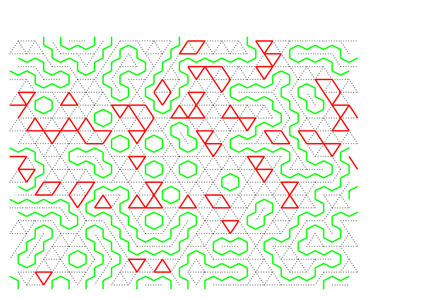
Figure 13: Snapshot of the bond coloring of lattice ${\mathcal{T}}(10)$. The lattice is a slab with a periodicity of $20$ lattice units in the horizontal direction and of finite width $L=20$ in the vertical direction. For greater clarity, instead of drawing the green bonds of ${\mathcal{T}}(10)$ themselves, we have drawn their duals. Most of the green chains form loops, but some are seen to be open-ended at the boundaries, in agreement with Corollary 14b. Each site of ${\mathcal{T}}(10)$ is joined by an even number, possibly zero, of red bonds. See text for more details.

5.5 Numerical evaluation

We have evaluated the ST evolution numerically for the slab depicted in figure 13. The top boundary advances and the bottom boundary recedes, the width $L$ remaining constant. The bond strengths $S_{i}^{(0)}(\vec{r})$ of the initial lattice $\mathcal{T}(0)$ were drawn independently from a zero-mean Gaussian distribution $N(S_{i})$ of width $\langle S_{i}^{2}\rangle^{1/2}=2$, so that all initial bonds were black. Figure 13 shows the bond colors of lattice ${\mathcal{T}}(10)$ that result after ten iterations with the uniform random protocol of section 4.3 applied at the top boundary. The green star legs form chains: a part of them are closed loops and another part begin and end at the top and/or bottom boundaries, in agreement with Corollary 14b.

6 Conclusion

The iterated star-triangle (ST) transformation is a tool that has led to various interesting results on 2D Ising systems. The transformation may be applied to triangular and hexagonal lattices with arbitrarily inhomogeneous nearest-neighbor couplings $K_{i}^{(0)}(\vec{r})$. To the best of our knowledge, however, there have not been, as of today, any applications to frustrated lattices, the difficulty being that in such lattices iteration may lead to complex-valued couplings. In this work we have addressed this problem.

We have found a general theorem, together with several corollaries, that is obeyed by systems that are subjected to iterated ST transformation (called in this work “ST evolution”). Our main result is that under ST evolution, when applied to an initial system with real-valued bond strengths $K_{i}^{(0)}(\vec{r})$, the variables $S_{i}^{(n)}(\vec{r})=1/\sinh 2K_{i}^{(0)}(\vec{r})$ that are generated successively will remain confined to the union of the real and the imaginary axis. This property is of interest in itself but it is also important for numerical applications. The result was shown to hold for systems which are infinite or have periodic boundary conditions, and also, when suitably reformulated, for half-infinite systems. In the latter the boundary behavior under ST evolution requires special attention and occupies a large place in this work. A distinction appears between receding and advancing boundaries: advancing ones require a protocol prescribing how new bonds at the boundary are created. We have shown that there is a class of random protocols that ensures the validity of the main result in the presence of an advancing boundary. Our method of proof attributes to each bond one out of three “colors,” black, red, or green, according to the value of its bond strength. Under ST evolution these colors obey rules that are instrumental in proving the theorems. One might think that our results ought to follow from a short and simple symmetry argument. If one exists, however, we think it would be unlikely to automatically cover the boundary behavior.

We illustrated our work by two brief numerical calculations, one for a lattice with periodic boundary conditions in both directions, and another one for a slab, periodic in only one direction and obeying a specific “uniform random” protocol along its advancing boundary.

We list a few interesting questions have not been answered. First, Section 4.3 shows that at an advancing boundary we have much freedom to define a protocol. In Section 5.5 we used the uniform random one, which is the first one to come to mind; but, can anything be gained from other protocols? And, well beyond the scope of this paper, would there be any advantage in employing protocols that do not  confine the $S_{i}^{(n)}(\vec{r})$ to the union ${\mathbb{R}}\cup{\rm i}{\mathbb{R}}$ of the two main axes in the complex plane? Secondly, there is the open question, mentioned in Section 3.6, of how to extract, with the aid of the present techniques, the zero-temperature exponents of the 2D Ising spin glass. Thirdly, there is a factor $\exp(g)$ that multiplies the partition function each time an ST transformation is applied. The study and the exploitation of this factor have been left aside in the present work, but certainly deserve attention; it enters, in particular, the calculation of free energies. Fourth, there are many quantitative numerical questions. How does an initial distribution of coupling strengths evolve? What is their asymptotic distribution, if any, when the number $n$ of iterations tends to infinity, and how does this depend on whether or not the lattice has a boundary?

We believe that the answer to several of these and to other questions, as well as specific applications, constitute an interesting direction of future research.

References

- [1] I. Syozi, in Phase Transitions and Critical Phenomena, edited by C. Domb and M.S. Green (Academic, London, 1972), Vol.1, p. 269.
- [2] L. Onsager, Phys. Rev. 65 (1944) 117.
- [3] G.H. Wannier, Rev. Mod. Phys. 17 (1945) 50.
- [4] R.M.F. Houtappel, Physica 16 (1950) 425.
- [5] H. Au-Yang and J.H.H. Perk, Advanced Studies in Pure Mathematics 19 (1989) 57.
- [6] J.H.H. Perk and H. Au-Yang, Encyclopedia of Mathematical Physics, eds. J.-P.-Françoise, G.L. Naber and S.T. Tsou, Oxford: Elsevier, 2006 (ISBN 978-0-1251-2666-3), volume 5, pages 465-473.
- [7] H.J. Hilhorst, M. Schick, and J.M.J. van Leeuwen, Phys. Rev. Lett. 40 (1978) 1605.
- [8] H.J. Hilhorst, M. Schick, and J.M.J. van Leeuwen, Phys. Rev. B 419 (1979) 2749.
- [9] H.J.F. Knops and H.J. Hilhorst, Phys.Rev. B 19 (1979) 3689.
- [10] Y. Yamazaki and H.J. Hilhorst, Phys. Lett. 70A (1979) 329.
- [11] Y. Yamazaki, G. Meissner, and H.J. Hilhorst, Z. Phys. B 35 (1979) 333.
- [12] Y. Yamazaki, H.J. Hilhorst, and G. Meissner, J. Stat. Phys. 23 (1980) 609.
- [13] H.J. Hilhorst and J.M.J. van Leeuwen, Phys. Rev. Lett. 47 (1981) 1188.
- [14] T.W. Burkhardt, Phys. Rev. Lett. 48 (1982) 216.
- [15] R. Cordery, Phys. Rev. Lett. 48 (1982) 215.
- [16] T.W. Burkhardt, I. Guim, H.J. Hilhorst, and J.M.J. van Leeuwen, Phys.Rev. B 30 (1984) 1486.
- [17] T.W. Burkhardt and I. Guim, Phys. Rev. B 29 (1984) 508(R).
- [18] T.W. Burkhardt and I. Guim, J. Phys. A 18 (1985) L33.
- [19] F. Iglói and P. Lajkó, J. Phys. A 29 (1996) 4803.
- [20] T.W. Burkhardt and I. Guim, Physica A 251 (1998) 12.
- [21] P. Lajkó and F. Iglói, Phys. Rev. E 61 (2000) 147.
- [22] B. Berche and L. Turban, J. Phys. A 23 (1990) 3029.
- [23] L. Turban, F. Iglói, and B. Berche, Phys. Rev. B 49 (1994) 12695.
- [24] W. Selke, F. Szalma, P. Lajkó, , and F. Iglói, J. Stat. Phys. 89 (1997) 1079.
- [25] F. Iglói, P. Lajkó, W. Selke, and F. Szalma, J. Phys. A 31 (1998) 2801.
- [26] L. Turban, D. Karevski, and F. Iglói, J. Phys. A 32 (1999) 3907.
- [27] D. Karevski, L. Turban, and F. Iglói, J. Phys. A 33 (2000) 2663.
- [28] L. Turban, Physica A 303 (2002) 275.
- [29] M. Collura, D. Karevski, and L. Turban, J. Stat. Mech. (2009) P08007.
- [30] F. Iglói, I. Peschel, and L. Turban, Advances in Physics 42 (1993) 683. Taylor & Francis.
- [31] A. Pelizzola, Int. J. Mod. Phys. B 11 (1997) 1363.
- [32] D.S. Fisher and D.A. Huse, Phys. Rev. Lett. 56 (1986) 1601.
- [33] D.S. Fisher and D.A. Huse, Phys. Rev. B 38 (1988) 386.
- [34] M.J. Thill and H.J. Hilhorst, J. Phys. I France 6 (1996) 67.