Background-Aware Pooling and Noise-Aware Loss for Weakly-Supervised Semantic Segmentation

Abstract

We address the problem of weakly-supervised semantic segmentation (WSSS) using bounding box annotations. Although object bounding boxes are good indicators to segment corresponding objects, they do not specify object boundaries, making it hard to train convolutional neural networks (CNNs) for semantic segmentation. We find that background regions are perceptually consistent in part within an image, and this can be leveraged to discriminate foreground and background regions inside object bounding boxes. To implement this idea, we propose a novel pooling method, dubbed background-aware pooling (BAP), that focuses more on aggregating foreground features inside the bounding boxes using attention maps. This allows to extract high-quality pseudo segmentation labels to train CNNs for semantic segmentation, but the labels still contain noise especially at object boundaries. To address this problem, we also introduce a noise-aware loss (NAL) that makes the networks less susceptible to incorrect labels. Experimental results demonstrate that learning with our pseudo labels already outperforms state-of-the-art weakly- and semi-supervised methods on the PASCAL VOC 2012 dataset, and the NAL further boosts the performance.

1 Introduction

(a) Input image.

(b) Ground truth.

(c) Ours.

(d) Ours^∗.

(e) GrabCut [48].

(f) MCG [44].

(g) WSSL [42].

(h) SDI [27].

Figure 1: Visual comparison of pseudo ground-truth labels. Our approach generates better segmentation labels than other WSSS methods using object bounding boxes (WSSL [42] and SDI [27]). Hand-crafted methods (GrabCut [48] and MCG [44]) fail to segment object boundaries. Ours^∗: Ours with an indication of unreliable regions. Best viewed in color.

Semantic segmentation is one of the fundamental tasks in computer vision, and has received a lot of attention over the last decades. It aims at assigning a semantic label to each pixel, which can be leveraged to various applications including scene understanding, autonomous driving, image editing, and robotics. Supervised methods based on convolutional neural networks (CNNs) [5, 40, 47] have achieved remarkable success in semantic segmentation, but they require lots of training samples with pixel-level labels, which are extremely labor-intensive to annotate, to train networks. Weakly-supervised semantic segmentation (WSSS) has recently been introduced to exploit a weak form of supervisory signals such as image-level labels [11, 14, 22, 28, 32, 56, 60], points [3], scribbles [35, 53, 54], and object bounding boxes [8, 27, 42, 52]. WSSS methods using image-level labels typically leverage class activation maps (CAMs) [63], obtained from CNNs for image classification using global average pooling (GAP), to localize objects. Since CAMs tend to highlight discriminative parts, these methods more or less resort to off-the-shelf saliency detectors [13, 21, 24, 33, 57]. This, however, requires additional pixel-level ground-truth annotations for salient objects. Other approaches attempt to exploit object bounding boxes. They are easy to annotate compared to pixel-level labels and provide rich semantics to localize objects. The object bounding boxes, however, contain a mixture of foreground and background, and do not specify exquisite object boundaries. To overcome this, recent approaches [8, 27, 31] use off-the-shelf segmentation methods [44, 48].

We introduce a simple yet effective WSSS method using bounding box annotations. In particular, we investigate two aspects of this problem – How can we generate high-quality but possibly noisy pixel-level labels (i.e., a pseudo ground truth) from object bounding boxes (Fig. 1)? How can we train CNNs for semantic segmentation (e.g., DeepLab [5, 6]) with noisy segmentation labels? Motivated by the methods using image-level labels [1, 22, 32, 55, 56], for the first aspect, we leverage a CNN for image classification, instead of exploiting off-the-shelf segmentation methods (e.g., [44, 48]). To this end, we propose a background-aware pooling (BAP) method using an attention map, enabling discriminating foreground and background inside the bounding boxes. This allows to aggregate features within a foreground for image classification, while discarding those for a background, resulting in more accurate CAMs, rather than mainly highlighting the most discriminative parts (e.g., faces in the person class) as in GAP [36, 63]. Specifically, we retrieve background regions inside the bounding boxes, based on our finding that background regions are perceptually consistent in part within an image. This provides attention maps for the background regions adaptively for individual images. We exploit the attention maps and CAMs, together with prototypical features, to generate pseudo ground-truth labels. For the second one, we introduce a noise-aware loss (NAL) to train CNNs for semantic segmentation that makes the networks less susceptible to incorrect labels. Specifically, we exploit a confidence map, using the distances between CNN features for prediction and classifier weights for semantic segmentation, to compute a cross-entropy loss adaptively. Experimental results demonstrate that our approach to using BAP already outperforms the state of the art on the PASCAL VOC 2012 dataset [10], and the NAL further boosts the performance. We also demonstrate the effectiveness of our approach by extending it to the task of instance segmentation on the MS-COCO dataset [38]. We summarize the contributions of our work as follows:

• We introduce a novel pooling method for WSSS, dubbed BAP, that uses bounding box annotations, allowing to generate high-quality pseudo ground-truth labels.

• We propose a NAL exploiting the distances between CNN features for prediction and classifier weights for semantic segmentation, lessening the influence of incorrect labels.

• We set a new state of the art on the PASCAL VOC 2012 dataset for weakly- and semi-supervised semantic segmentation. We also provide an extensive experimental analysis with ablation studies.

Our code and models are available online: https://cvlab.yonsei.ac.kr/projects/BANA.

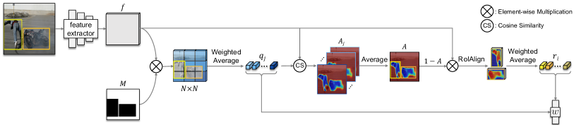
Figure 2: Overview of image classification using BAP. We first extract queries $q_{j}$ using a feature map $f$ and a binary mask $M$ indicating a definite background. The queries $q_{j}$ are then used to compute an attention map $A$ describing the likelihood that each pixel belongs to a background. The attention map enables localizing entire foreground regions, leading to better foreground features $r_{i}$. Finally, we apply a softmax classifier $w$ to the foreground features $r_{i}$ for each bounding box together with the queries $q_{j}$. The entire network is trained with a cross-entropy loss. See text for details (Sec. 3.1). Best viewed in color.

2 Related work

WSSS using image-level labels. Image-level labels have been used for WSSS as an alternative to dense pixel-level annotations. However, they indicate the presence or absence of objects of a particular class only, and do not provide any information for the location of objects, making the problem extremely challenging. The seminal work of [63] proposes CAMs to estimate coarse localization maps for objects or actions by using a CNN trained with the image-level labels. Since then, several WSSS methods exploit CAMs to generate a pseudo ground truth, which is used to train CNNs for semantic segmentation in a supervised manner, by propagating them with DenseCRF [23, 28, 49, 60], using a stochastic inference [32], incorporating a self-supervised task [4], or alternatively mining and erasing object-related regions [22, 34, 55, 56]. These approaches enlarge initial CAMs, typically activated on the most discriminative parts, progressively to cover entire objects, but this may highlight the regions irrelevant to objects (e.g., a background). To address this problem, off-the-shelf saliency detectors [13, 21, 24, 33, 57] and/or segment proposals [7, 44] have been used, but they require calibrating saliency/objectness scores carefully. SSNet [59] proposes to learn WSSS and saliency detection jointly with a unified network architecture, but it requires ground-truth saliency annotations. Unlike these methods using image-level labels, we require no external models nor ground-truth saliency annotations. Recently, SeeNet [22] proposes to use background regions for WSSS. It defines a background explicitly using CAMs whose values are below a threshold, and prevents spreading CAMs into the background. Our work is similar to SeeNet in that both exploit the background regions. Differently, we define the background regions implicitly using a nonparametric retrieval technique, with an assumption that the background is perceptually consistent in part within an image. We then leverage them to design a new pooling method and to generate pseudo ground-truth labels.

WSSS using bounding box labels. An alternative approach for WSSS is to exploit object bounding boxes as a supervisory signal. They are easy to annotate compared to pixel-level labels (e.g., annotating boxes is about 15 times cheaper than labeling pixel-wise segments [38]), and provide a definite background with the extent of each object. In this context, recent methods [8, 27, 31, 42, 52] close the performance gap between weakly-supervised and fully-supervised methods. For example, BoxSup [8] employs MCG [44] to generate candidate segments and uses object bounding boxes to update the segments iteratively along with network parameters. WSSL [42] adopts DenseCRF [29] to generate pseudo segmentation labels using bounding boxes, and proposes an expectation-maximization algorithm to refine the labels. SDI [27] argues that generating correct pseudo labels is a crucial step for the performance of WSSS, and proposes to use GrabCut [48] and MCG to estimate the labels. We also advocate the importance of high-quality pseudo labels for WSSS, but exploit a classification network, similar to the methods using image-level labels, instead of exploiting the off-the-shelf segmentation methods [44, 48] or additional datasets [2].

Learning from noisy labels. Several methods have been proposed for correcting or filtering out noisy labels, e.g., [25, 41, 46, 50, 61] to name a few. We refer to [15] for a comprehensive review. In the context of WSSS, pseudo ground-truth labels generated by a weak form of supervisory signals are not accurate compared to manual annotations, making the task much more difficult. To alleviate the influence of noisy segmentation labels, SDI [27] discards regions whose labels obtained by MCG [44] and GrabCut [48] are different, to train a network. Similarly, the work of [12] exploits multiple pseudo labels that might complement each other. This work, however, requires 12 different pseudo labels obtained from two classification networks. By contrast, we generate two pseudo labels with a negligible overhead. Recently, BCM [52] introduces a filling rate constraint. It filters out incorrectly labeled pixels, based on the mean percentage of foreground pixels within bounding boxes of each object class. Box2Seg [31] also uses the filling rate constraint to regularize a class-specific attention map. The attention map is then used to modulate a cross-entropy loss to handle incorrect labels. These approaches [31, 52] outperform other methods, but require a pre-training stage to stabilize the training and use additional parameters to compute losses, which is in contrast to our NAL.

3 Approach

Our approach mainly consists of three stages: First, we train a CNN for image classification using object bounding boxes (Fig. 2). We use BAP leveraging a background prior, that is, background regions are perceptually consistent in part within an image, allowing to extract more accurate CAMs. To this end, we compute an attention map for a background adaptively for each image. Second, we generate pseudo segmentation labels using CAMs obtained from the classification network together with the background attention maps and prototypical features (Fig. 3). Finally, we train CNNs for semantic segmentation with the pseudo ground truth but possibly having noisy labels. We use a NAL to lessen the influence of the noisy labels. In the following, we describe a detailed description of each stage.

3.1 Image classification using BAP

Our classification network consists of a feature extractor and a ($L+1$)-way softmax classifier ($L$ object classes and the background class). Given an input image, the feature extractor outputs a feature map $f$. We denote by $\mathcal{B}=\{B_{1},B_{2},\dots,B_{K}\}$ a set of object bounding boxes in the input image, where $K$ is the number of bounding boxes, resized w.r.t. the size of the feature map $f$ correspondingly using nearest-neighbor interpolation. We denote by $M$ a mask indicating a definite background (i.e., the regions outside the bounding boxes), where $M(\mathbf{p})=1$ if the position $\mathbf{p}$ does not belong to any bounding boxes, and $M(\mathbf{p})=0$ otherwise.

Background attention map. Separating foreground and background regions inside object bounding boxes allows the classifier to focus more on learning foreground objects. As will be seen in our experiments, this results in better CAMs localizing entire objects. However, the object bounding boxes contain a mixture of foreground and background, and do not provide any information about object boundaries. To discriminate foreground and background regions for each bounding box, we pose this problem as a retrieval task. Specifically, we divide the feature map $f$ into $N\times N$ regular grids. We denote by $G(j)$ each grid cell, where $1\leq j\leq N^{2}$. Note that we ignore invalid cells that do not overlap with the definite background regions at all, (i.e., the cells inside object bounding boxes), suggesting that each input image could have different numbers of valid grid cells, at most $N^{2}$. We then aggregate features for individual grid cells, and use them as queries for retrieval as follows:

$$q_{j}=\frac{\displaystyle\sum_{\mathbf{p}\in G(j)}M(\mathbf{p})f(\mathbf{p})}{\displaystyle\sum_{\mathbf{p}\in G(j)}M(\mathbf{p})}.$$ (1)

That is, we obtain individual queries $q_{j}$ by computing a weighted average of features $f$ on corresponding grid cell $G(j)$ using the binary mask $M$. Given the queries, we retrieve the background regions inside the bounding boxes, and obtain an attention map $A$ as follows:

$$A(\mathbf{p})=\frac{1}{J}\sum_{j}A_{j}(\mathbf{p}),$$ (2)

where $J$ is the number of valid grid cells and

$$A_{j}(\mathbf{p})=\left\{\begin{matrix}\text{ReLU}\left(\frac{f(\mathbf{p})}{\|f(\mathbf{p})\|}\cdot\frac{q_{j}}{\|q_{j}\|}\right)&,\mathbf{p}\in\mathcal{B}\\ 1&,\mathbf{p}\notin\mathcal{B}\end{matrix}\right..$$ (3)

We denote by $\|\cdot\|$ L2 normalization. This computes cosine similarity between features inside the bounding boxes $\mathcal{B}$ and queries $q_{j}$, and truncates the results into the range of $[0,1]$ by the ReLU [30] function. Accordingly, the attention map $A$ quantifies the likelihood that each pixel inside the bounding boxes belongs to a background. It is more likely to be a background, as the value of the attention map $A$ approaches to one.

BAP. We use the attention map $A$ to aggregate foreground features for each bounding box $B_{i}$ as follows:

$$r_{i}=\frac{\displaystyle\sum_{\mathbf{p}\in B_{i}}(1-A(\mathbf{p}))f(\mathbf{p})}{\displaystyle\sum_{\mathbf{p}\in B_{i}}(1-A(\mathbf{p}))},$$ (4)

which corresponds to weighted average pooling, where the weight is the probability of the point at $\mathbf{p}\in B_{i}$ being a foreground. Note that it becomes GAP, when all regions inside the bounding box are considered as a foreground (i.e., $A=0$).

Loss. We apply the ($L+1$)-way softmax classifier $w$ to individual features for the foreground and background regions (i.e., $r_{i}$ and $q_{j}$, respectively) to train the classification network with a standard cross-entropy loss. This enables better distinguishing foreground objects from a background.

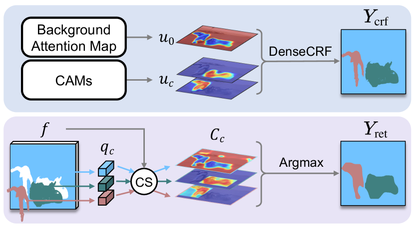
Figure 3: Generating pseudo labels. We compute $u_{0}$ and $u_{c}$ using a background attention map and CAMs, respectively, which are used as a unary term for DenseCRF [29] to obtain pseudo segmentation labels $Y_{\text{crf}}$. We extract prototypical features $q_{c}$ for each class using the labels $Y_{\text{crf}}$, and use them as queries to retrieve high-level features from the feature map $f$, from which we obtain additional pseudo labels $Y_{\text{ret}}$. See text for detail (Sec. 3.2). Best viewed in color.

3.2 Pseudo label generation

We introduce two approaches, complementary to each other, to generate pseudo ground-truth labels. First, we leverage CAMs for each object bounding box obtained from the classification network using BAP. We exploit DenseCRF [29] with a unary term for each object class $c$ defined as:

$$u_{c}(\mathbf{p})=\left\{\begin{matrix}\frac{\text{CAM}_{c}(\mathbf{p})}{\max_{\mathbf{p}}(\text{CAM}_{c}(\mathbf{p}))}&,\mathbf{p}\in\mathcal{B}_{c}\\ 0&,\mathbf{p}\notin\mathcal{B}_{c}\end{matrix}\right.,$$ (5)

where we denote by $\mathcal{B}_{c}$ a set of bounding boxes containing objects of the class $c$ and

$$\text{CAM}_{c}(\mathbf{p})=\text{ReLU}(f(\mathbf{p})\cdot w_{c}).$$ (6)

$w_{c}$ is the classifier weight for the object class $c$. For the background class, we use the background attention map $A$ as follows:

$$u_{0}(\mathbf{p})=A(\mathbf{p}).$$ (7)

Note that we could also use the CAM for the background class directly, similar to other object classes, but it highlights the most frequently observed regions in the dataset during training, lessening the discriminative ability of CRF to separate foreground and background inside the bounding boxes. For a pairwise term, we follow other WSSS methods that use contrast-sensitive bilateral potentials using color values and positions as in [29]. We concatenate the unary terms for each object class in Eq. (5) and the background in Eq. (7), and input them to DenseCRF together with an input image to obtain segmentation labels $Y_{\text{crf}}$. Second, while the first approach using DenseCRF delineates object boundaries, low-level features (e.g., color and texture) in the pairwise term might result in incorrect segmentation labels. We thus leverage high-level features $f$ obtained from the classification network to complement this. Specifically, we propose to use a retrieval technique similar to BAP. We extract a prototypical feature for each class as follows:

$$q_{c}=\frac{1}{|\mathcal{Q}_{c}|}{\displaystyle\sum_{\mathbf{p}\in\mathcal{Q}_{c}}f(\mathbf{p})},$$ (8)

where $\mathcal{Q}_{c}$ is a set of locations labeled as the class $c$ in $Y_{\text{crf}}$ (including the background class) and $|\cdot|$ indicates the number of pixels. We use prototypical features as queries to retrieve similar ones from the feature map $f$, and compute a correlation map for each class as follows:

$$C_{c}(\mathbf{p})=\frac{f(\mathbf{p})}{\|f(\mathbf{p})\|}\cdot\frac{q_{c}}{\|q_{c}\|}.$$ (9)

We then obtain pseudo segmentation labels $Y_{\text{ret}}$ by applying the argmax function over the correlation maps $C_{c}$.

3.3 Semantic segmentation with noisy labels

We train DeepLab [5, 6] for semantic segmentation with the pseudo pixel-level labels, $Y_{\text{crf}}$ and $Y_{\text{ret}}$. We extract a feature map $\phi$ from the penultimate layer, and pass it through a softmax classifier $W$, resulting in a $(L+1)$-dimensional probability map $H$. To alleviate the influence of incorrect labels, we exploit the regions $\mathcal{S}$, where both $Y_{\text{crf}}$ and $Y_{\text{ret}}$ give the same label, to compute the loss as follows:

$$\mathcal{L}_{\text{ce}}=-\frac{1}{\sum_{c}|\mathcal{S}_{c}|}\sum_{c}\sum_{\mathbf{p}\in\mathcal{S}_{c}}\log H_{c}(\mathbf{p}),$$ (10)

where $H_{c}$ is a probability for the class $c$, and $\mathcal{S}_{c}$ is a set of locations labeled as the class $c$ in $\mathcal{S}$. We also exploit other regions ${\sim}\mathcal{S}$, where $Y_{\text{crf}}$ and $Y_{\text{ret}}$ give different labels, rather than discarding them completely as in [27]. These regions are less reliable than $\mathcal{S}$, but might contain correct labels. It is, however, hard to determine whether the label is correct or not. Motivated by the work of [39, 45], we assume that a classifier weight represents a center of each class in the feature space, suggesting that the weight can be thought of as a representative feature for the corresponding class. We thus distinguish the label noise by using the distances between CNN features and classifier weights. To implement this idea, we first compute a correlation map for each class as follows:

$$D_{c}(\mathbf{p})=1+\left(\frac{\phi(\mathbf{p})}{\|\phi(\mathbf{p})\|}\cdot\frac{W_{c}}{\|W_{c}\|}\right),$$ (11)

where we denote by $W_{c}$ the classifier weight for the corresponding class $c$. We use cosine similarity as a metric with adding one to force the correlation score to be positive. We then compute a confidence map as follows:

$$\sigma(\mathbf{p})=\left(\frac{D_{c^{*}}(\mathbf{p})}{\max_{c}(D_{c}(\mathbf{p}))}\right)^{\gamma},$$ (12)

where $c^{*}$ is a label obtained by $Y_{\text{crf}}$ (i.e., $c^{*}=Y_{\text{crf}}(\mathbf{p})$), and $\gamma~{}(\geq 1)$ is a damping parameter. The confidence map provides the likelihood of each label being correct. The rationale for this is that the correlation values of $D_{c^{*}}(\mathbf{p})$ and $\max_{c}(D_{c}(\mathbf{p}))$ will be similar, when the label $c^{*}$ is confident, and vice versa. Note that we can adjust the confidence values with the damping parameter $\gamma$. When $\gamma$ approaches to infinity, the values become binary, considering the most confident labels only and acting as a hard constraint. That is, $\sigma(\mathbf{p})=1$ only when $D_{c^{*}}(\mathbf{p})=\max_{c}(D_{c}(\mathbf{p}))$, and $\sigma(\mathbf{p})\approx 0$ otherwise. We exploit the confidence map as a weighting factor to compute the cross-entropy loss as follows:

$$\mathcal{L}_{\text{wce}}=-\frac{1}{\sum_{c}\sum_{\mathbf{p}\in\mathcal{{\sim}S}_{c}}\sigma(\mathbf{p})}\sum_{c}\sum_{\mathbf{p}\in\mathcal{{\sim}S}_{c}}\sigma(\mathbf{p})\,\log H_{c}(\mathbf{p}),$$ (13)

where we denote by ${\sim}\mathcal{S}_{c}$ a set of location labeled as the class $c$ in ${\sim}\mathcal{S}$. Accordingly, the overall NAL is defined with a balance parameter $\lambda$ as follows:

$$\mathcal{L}=\mathcal{L}_{\text{ce}}+\lambda\,\mathcal{L}_{\text{wce}}.$$ (14)

4 Experiments

In this section, we describe implementation details, and present a detailed analysis of our method with ablation studies. We then compare our model with state-of-the-art WSSS methods. We obtain experimental results using PyTorch [43] with a NVIDIA Titan RTX GPU. More results including qualitative comparisons can be found in the supplementary material.

4.1 Implementation details

Dataset and evaluation. We use the PASCAL VOC 2012 dataset [10] consisting of $1,464$/$1,449$/$1,456$ samples of 21 classes (including the background class) for $train$, $val$, and $test$, respectively. Following the common practice in [8, 28, 32, 52], we use augmented $10,582$ training samples provided by [18] to train our models. We use the mean intersection-over-union (mIoU) metric to measure the precision of pseudo segmentation labels and segmentation results. We obtain results for the $test$ set on the official PASCAL VOC evaluation server. For instance segmentation, we use MS-COCO [38] for 115K/5K/20K samples of $train$, $val$, and $test$, respectively, containing 81 classes including the background class. We use the average precision (AP) metrics to evaluate pseudo labels and segmentation results.

Classification network. We adopt the classification network in AffinityNet [1], a slight modification of VGG-16 [51] pre-trained for ImageNet classification [9], to extract the feature map $f$. Initially, classifier weights are sampled randomly from a Gaussian distribution with zero mean and standard deviation of 1e-2. We train the classification network for 15 epochs with a batch size of 20 using the SGD optimizer with momentum of $0.9$ and weight decay of 5e-4. Learning rates are initially set to 1e-4 and 1e-3 for the pre-trained layers and the classifier, respectively, and they are divided by 10 after 10 epochs. We augment the training set with horizontal flipping, random cropping ($321\times 321$), random scaling, and color jittering.

Segmentation network. For fair comparison, we exploit two models for semantic segmentation: DeepLab-V1 (LargeFOV) [5, 6] with VGG-16 [51] and DeepLab-V2 (ASPP) [6] with ResNet-101 [20]. We train DeepLab-V1 (V2) for 45 (20) epochs with a batch size of 20 (10), and adjust the learning rate using the poly schedule [6].

Hyperparameter settings. Following the experimental protocol in [8, 42], parameters for DenseCRF [29] are chosen by cross-validation on the held-out set of 100 validation images fully-annotated. We set the grid size $N$ to 4 for training a classification network using BAP in order to see diverse background queries. We empirically find that using confident background regions in Eq. (7), that is, thresholding $A$ with $0.99$, and setting $N$ to 1 provide better results when generating pseudo labels. We use a grid search to set the threshold value for $A$ and the grid size $N$ on the same held-out set for DenseCRF. For DeepLab, we use default settings in [5, 6]. Other parameters are fixed to all experiments ($\gamma=7,~{}\lambda=0.1$). In the supplementary material, we provide quantitative comparisons and more analysis on these parameters.

4.2 Analysis

Table 1: Comparison of pseudo labels on the PASCAL VOC 2012 [10] $train$ and $val$ sets in terms of mIoU. Numbers in bold indicate the best performance. We report the supervision types with the number of annotations. For MCG [44], we manually choose the segment proposal that gives the highest IoU score with each bounding box. ^∗: pseudo labels contain unreliable regions.

Method	$train$	$val$
Supervision: Image-level labels (10K)
AffinityNet${}_{\text{CVPR'18}}$ [1]	59.7	-
Supervision: Boxes (10K)
Box	65.4	62.2
GrabCut${}_{\text{TOG'04}}$ [48]	65.7	66.1
MCG${}_{\text{PAMI'16}}$ [44]	66.2	66.9
WSSL${}_{\text{ICCV'15}}$ [42]	69.7	71.1
SDI${}_{\text{CVPR'17}}$ [27]	79.7∗	60.5∗
Ours
GAP	75.5	76.1
BAP: $Y_{\text{crf}}$ w/o $u_{0}$	77.0	77.8
BAP: $Y_{\text{crf}}$	78.7	79.2
BAP: $Y_{\text{ret}}$	70.8	69.9
BAP: $Y_{\text{crf}}$ & $Y_{\text{ret}}$	85.3∗	68.2∗

Table 2: Comparison of pseudo labels on the MS-COCO [38] $train$ set. Note that the results for ‘VOC-to-COCO’ do not use any samples in the MS-COCO $train$ set during training.

Method	AP	$\text{AP}_{50}$	$\text{AP}_{75}$	$\text{AP}_{S}$	$\text{AP}_{M}$	$\text{AP}_{L}$
VOC-to-COCO
BAP: $Y_{\text{crf}}$	11.7	28.7	8.0	3.0	15.0	27.1
BAP: $Y_{\text{ret}}$	9.0	30.1	2.8	4.4	10.2	16.2
COCO-to-COCO
BAP: $Y_{\text{crf}}$	17.2	40.5	12.5	5.9	20.4	32.2
BAP: $Y_{\text{ret}}$	17.2	49.7	7.6	12.0	17.1	22.5

Accuracy of pseudo labels. We compare in Table 1 mIoU scores of pseudo segmentation labels on the PASCAL VOC 2012 [10] $train$ and $val$ sets. Note that our pseudo label generator can segment foreground objects given bounding boxes, even for unseen images during training. To the baseline, we consider the bounding box itself as a foreground object (‘Box’), which outperforms AffinityNet [1] using image-level labels. This suggests that the bounding box is a strong indicator for segmenting objects. WSSL [42] using DenseCRF [29] outperforms the baseline and hand-crafted methods [44, 48] by a considerable margin. To validate our approach to using a classification network with bounding boxes, we train a CNN with GAP for image classification, and generate pseudo labels using CAMs and DenseCRF (‘GAP’). We can clearly see that this approach already outperforms WSSL significantly, demonstrating the effectiveness of our approach. GAP, however, does not discriminate foreground and background regions inside bounding boxes. BAP overcomes this problem, and provides better CAMs, resulting in more accurate pseudo labels (‘BAP: $Y_{\text{crf}}$’). Note that BAP does not introduce any additional parameters, similar to GAP. For comparison, we generate pseudo labels by replacing the background attention map $u_{0}$ in Eq. (7) with the CAM for the background class (‘BAP: $Y_{\text{crf}}$ w/o $u_{0}$’), the performance of which is lower than ‘BAP: $Y_{\text{crf}}$’. A plausible explanation is that the CAM for the background class highlights the most frequently observed regions only. In contrast to this, the attention map $u_{0}$, a by-product of our BAP, marks background regions adaptively for individual images. We also report the mIoU scores for the pseudo labels obtained by a retrieval technique (‘BAP: $Y_{\text{ret}}$’). Although this provides worse results than ‘BAP: $Y_{\text{crf}}$’, due to the use of the low-resolution feature map $f$, as will be shown later, they are complementary to each other. Note that both pseudo labels of SDI [27] and ours (‘BAP: $Y_{\text{crf}}$ & $Y_{\text{ret}}$’) contain unreliable regions as shown in Fig. 1, making it hard to compare them with other methods. ‘BAP: $Y_{\text{crf}}$ & $Y_{\text{ret}}$’ show better results than SDI, but this should not be considered as fair comparison since performance would be different depending on the quantity of unreliable regions.

Our pseudo label generator is generic in that the adaptive attention map $u_{0}$ allows to segment foreground objects for unseen classes during training. For example, even if we do not have a classifier weight for a novel class (see Eq. (6)), we can exploit $1-u_{0}$ as a class-agnostic foreground attention map. To validate this, we perform a cross-dataset evaluation in Table 2, where we generate pseudo labels on the MS-COCO [38] $train$ set by using the generator trained on PASCAL VOC 2012 [10] (‘VOC-to-COCO’). For comparison, we train and evaluate our generator on the same dataset (‘COCO-to-COCO’). From this table, we observe three things: (1) VOC-to-COCO gives reasonable pseudo labels even though it does not use any training samples of COCO during training. This is because our model computes the attention map adaptively, allowing to handle unseen object classes; (2) Two pseudo labels, $Y_{\text{crf}}$ and $Y_{\text{ret}}$, are complementary to each other. For example, $Y_{\text{ret}}$ gives better results for small objects, while $Y_{\text{crf}}$ performs better for large objects; (3) COCO-to-COCO provides better results, demonstrating the flexibility of our approach.

Comparison of CAMs. To verify that our BAP improves the quality of CAMs, we provide visual examples of CAMs in Fig. 4(a). We can clearly see that our BAP localizes the entire extent of objects (e.g., man’s legs in the first example) and does not highlight the irrelevant regions (e.g., airstrip in the third example). Quantitative comparisons of BAP and GAP in terms of the precision of CAMs and classification performance can be found in the supplementary material.

(a) Input.

(b) GAP.

(c) BAP.

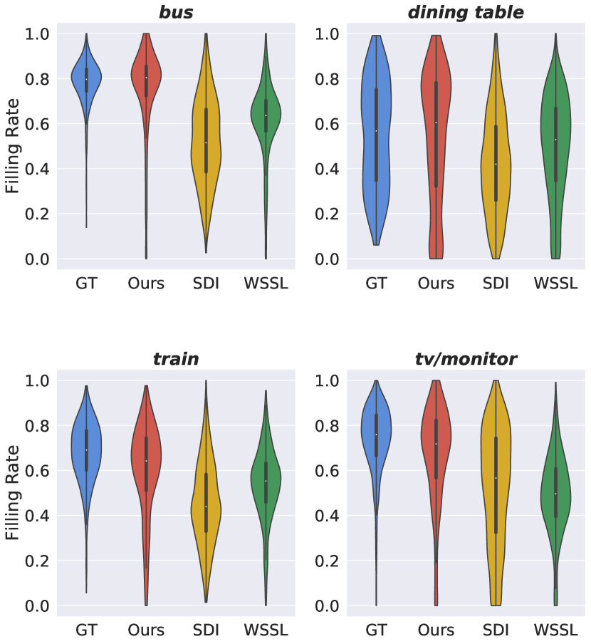
(a) CAMs.

(b) Violin plots of filling rate.

Figure 4: (a) Visual comparison of CAMs using GAP and BAP. Our model using BAP provides better CAMs, highlighting the entire objects while suppressing irrelevant regions. (b) Comparison of filling rate distributions on the PASCAL VOC 2012 [10] $train$ set. Best viewed in color.

Comparison of filling rates. Recent methods [31, 52] show that a filling rate, the percentage of foreground pixels inside the bounding box, can be a good indicator to select the most confidence regions for back propagation. They use GrabCut [48] to generate pseudo labels, and adopt the labels from WSSL [42], respectively. The per-class filling rates computed with these methods, however, vary significantly, and they are far from the ground truth. We show in Fig. 4(b) examples of violin plot distributions for filling rates. We compare the filling rates estimated by SDI [27], WSSL, ours, and the ground truth. We can see that the filling rates generated by our pseudo labels are more closer to the ground truth than other methods. We expect that our pseudo labels could improve the performance of other WSSS methods using the filling rate.

Table 3: Comparison of mIoU scores using different losses for the regions, ${\sim}\mathcal{S}$, where $Y_{\text{crf}}$ and $Y_{\text{ret}}$ give different labels, on the PASCAL VOC 2012 [10] $val$ set. We provide both mIoU scores before/after applying DenseCRF [29].

Method	$val$
Baseline	61.8 / 67.5
w/ Entropy Regularization [17]	61.4 / 67.3
w/ Bootstrapping [46]	61.9 / 67.6
w/ $\mathcal{L}_{\text{wce}}$ (Eq. $\eqref{eq:wce}$)	62.4 / 68.1

(a) Input image.

(b) Ours.

(c) Ours^∗.

(d) Ground truth.

Confidence maps $\sigma$.

Figure 5: Visual comparison of our pseudo labels $Y_{\text{crf}}$, the same ones but with an indication of unreliable regions using $Y_{\text{ret}}$, and the ground truth for the input image (top). Visualization of confidence maps at (from left to right) 0, 11, 22, 33 and 45 epochs (bottom). Best viewed in color.

NAL. We show in Table 3 mIoU scores of DeepLab-V1 [5] using different losses for regions ${\sim}\mathcal{S}$, where $Y_{\text{crf}}$ and $Y_{\text{ret}}$ give different labels. To the baseline, we ignore ${\sim}\mathcal{S}$ completely as in [27]. We can see that a bootstrapping technique [46] boosts the mIoU performance slightly, while an entropy regularization method [17] does not. Our NAL penalizes incorrect labels adaptively, achieving the best result. This suggests that some pseudo labels in the regions ${\sim}\mathcal{S}$ are correct and exploiting them can boost the performance. We compare in Fig. 5 our pseudo labels with the ground truth, and visualize an evolution of the confidence map in Eq. (12) during training. As the input image contains two different objects having similar color, i.e., dark stripes and a dog, our pseudo labels $Y_{\text{crf}}$ are incorrect for the stripes, which could be, however, marked with $Y_{\text{ret}}$. We can also see that our NAL assigns low confidence scores to the stripes, while maintaining high scores for the dog’s legs.

4.3 Segmentation results

PASCAL VOC. We compare in Table 4 the mIoU performance of our approach and state-of-the-art methods using DeepLab-V1 [5, 6]. We can see that our model trained with $Y_{\text{crf}}$ already outperforms the state of the art by a significant margin without altering the training scheme [5, 6]. This demonstrates that our approach to using a classification network with bounding boxes could be a promising way to generate a pseudo ground truth. We can also see that exploiting both labels, $Y_{\text{crf}}$ and $Y_{\text{ret}}$, together with our NAL further boosts the performance. We also report results for semi-supervised semantic segmentation. Following the experimental protocol in [8, 27, 42, 52], we use ground-truth segmentation labels of $1,464$ images in the original $train$ set (13.8% of the total images). Our method again achieves the best performance on the $val$ and $test$ sets.

We report in Table 5 segmentation results using DeepLab-V2 [6]. It shows that we can achieve higher mIoU scores with a deeper CNN. The behavior of mIoU scores is almost the same as the one for DeepLab-V1 in Table 4. Our model trained with $Y_{\text{ret}}$ even outperforms BCM [52] in this case. This suggests that our pseudo labels are more likely to be exploited by deeper CNNs, further demonstrating the importance of high-quality pseudo labels for WSSS. Although Box2Seg [31] gives the best performance, it adopts UPerNet [58] which requires a feature pyramid network [37] (FPN), a pyramid pooling module [62] (PPM), and additional decoders. Note that UPerNet yields performance similar to PSPNet [62] that outperforms DeepLab-V2 significantly.

MS-COCO. We show in Table 6 a quantitative comparison of our models and other methods for instance segmentation. To this end, we train Mask-RCNN [19] with our pseudo labels. Since Mask-RCNN uses a binary cross-entropy loss for each object class, we could not obtain the correlation map in Eq. (11). We thus compute the loss for the regions $\mathcal{S}$ only. For comparison, we report results of Mask-RCNN trained with ground-truth segmentation labels. From this table, we can see that Mask-RCNN trained with VOC-to-COCO outperforms AISI [14], demonstrating that the generalization ability of our method. Note that AISI generates a pseudo ground truth using image-level labels, but requires the instance-level saliency detector [13] trained with ground-truth saliency annotations. Our model trained on COCO-to-COCO outperforms the other one using VOC-to-COCO, demonstrating again the importance of high-quality pseudo labels (see the results in Table 2).

Table 4: Quantitative comparison with state-of-the-art methods using DeepLab-V1 (VGG-16) [5, 6] on the PASCAL VOC 2012 [10] dataset in terms of mIoU. Numbers in bold indicate the best performance and underscored ones are the second best.

Method	$val$	$test$
Supervision: Image-level labels (10K) with Saliency (3K)
SeeNet${}_{\text{NIPS'18}}$ [22]	61.1	60.7
FickleNet${}_{\text{CVPR'19}}$ [32]	61.2	61.9
OAA${}_{\text{ICCV'19}}$ [26]	63.1	62.8
ICD${}_{\text{CVPR'20}}$ [11]	64.0	63.9
Supervision: Boxes (10K)
BoxSup${}_{\text{ICCV'15}}$ [8]	62.0	64.6
WSSL${}_{\text{ICCV'15}}$ [42]	60.6	62.2
SDI${}_{\text{CVPR'17}}$ [27]	65.7	67.5
BCM${}_{\text{CVPR'19}}$ [52]	66.8	-
Ours
w/ $Y_{\text{crf}}$	67.8	-
w/ $Y_{\text{ret}}$	66.1	-
w/ NAL	68.1	69.4
Supervision: Boxes (9K) with Masks (1K)
BoxSup${}_{\text{ICCV'15}}$ [8]	63.5	66.2
WSSL${}_{\text{ICCV'15}}$ [42]	65.1	66.6
SDI${}_{\text{CVPR'17}}$ [27]	65.8	66.9
BCM${}_{\text{CVPR'19}}$ [52]	67.5	-
Ours w/ NAL	70.5	71.5

Table 5: Quantitative comparison with state-of-the-art methods using DeepLab-V2 (ResNet-101) [6] on the PASCAL VOC 2012 [10] dataset in terms of mIoU. Numbers in bold indicate the best performance and underscored ones are the second best. Contrary to others, Box2Seg [31] adopts UPerNet [58] that consists of the FPN [37], the PPM [62], and three decoders. ^†: models using pre-trained weights on MS-COCO [38]. ^∗: models using 10% of the total images with ground-truth segmentation labels.

Method	$val$	$test$
Supervision: Image-level labels (10K) with Saliency (3K)
SeeNet${}_{\text{NIPS'18}}$ [22]	63.1	62.8
FickleNet${}_{\text{CVPR'19}}$ [32]	64.9	65.3
OAA${}_{\text{ICCV'19}}$ [26]	65.2	66.4
ICD${}_{\text{CVPR'20}}$ [11]	67.8	68.0
Supervision: Boxes (10K)
SDI${}^{\dagger}_{\text{CVPR'17}}$ [27]	74.2	-
BCM${}^{\dagger}_{\text{CVPR'19}}$ [52]	70.2	-
Box2Seg${}_{\text{ECCV'20}}$ [31]	76.4	-
Ours†
w/ $Y_{\text{crf}}$	74.0	-
w/ $Y_{\text{ret}}$	72.4	-
w/ NAL	74.6	76.1
Supervision: Boxes (9K) with Masks (1K)
BCM${}^{\dagger}_{\text{CVPR'19}}$ [52]	71.6	-
Box2Seg${}^{*}_{\text{ECCV'20}}$ [31]	83.1	-
Ours† w/ NAL	78.7	79.4

Table 6: Quantitative comparison for instance segmentation on the MS-COCO [38] $test$ set.

Method	AP	$\text{AP}_{50}$	$\text{AP}_{75}$	$\text{AP}_{S}$	$\text{AP}_{M}$	$\text{AP}_{L}$
Mask-RCNN [19]	35.7	58.0	37.8	15.5	38.1	52.4
AISI [14]	13.7	25.5	13.5	0.7	15.7	26.1
Ours (‘VOC-to-COCO’)	16.9	38.2	13.0	7.3	17.1	26.5
Ours (‘COCO-to-COCO’)	22.2	47.1	18.7	11.2	22.1	31.4

5 Conclusion

We have presented a novel pooling method for WSSS, dubbed BAP, using a background prior, that discriminates foreground and background regions inside object bounding boxes. We have shown that our BAP allows to produce better pseudo ground-truth labels compared to the conventional GAP. We have proposed a NAL for training a segmentation network, making it less susceptible to incorrect pseudo labels. Finally, we have shown that our approach achieves state-of-the-art performance on PASCAL VOC and MS-COCO.

Acknowledgments. This work was supported by the National Research Foundation of Korea (NRF) grant funded by the Korea government (MSIP) (NRF-2019R1A2C2084816).

See pages 1 of 04630-supp.pdf See pages 2 of 04630-supp.pdf See pages 3 of 04630-supp.pdf See pages 4 of 04630-supp.pdf See pages 5 of 04630-supp.pdf See pages 6 of 04630-supp.pdf See pages 7 of 04630-supp.pdf See pages 8 of 04630-supp.pdf See pages 9 of 04630-supp.pdf

References

- [1] Jiwoon Ahn and Suha Kwak. Learning pixel-level semantic affinity with image-level supervision for weakly supervised semantic segmentation. In CVPR, 2018.
- [2] Pablo Arbelaez, Michael Maire, Charless Fowlkes, and Jitendra Malik. Contour detection and hierarchical image segmentation. IEEE Trans. PAMI, 33(5):898–916, 2010.
- [3] Amy Bearman, Olga Russakovsky, Vittorio Ferrari, and Li Fei-Fei. What’s the point: Semantic segmentation with point supervision. In ECCV, 2016.
- [4] Yu-Ting Chang, Qiaosong Wang, Wei-Chih Hung, Robinson Piramuthu, Yi-Hsuan Tsai, and Ming-Hsuan Yang. Weakly-supervised semantic segmentation via sub-category exploration. In CVPR, 2020.
- [5] Liang-Chieh Chen, George Papandreou, Iasonas Kokkinos, Kevin Murphy, and Alan L Yuille. Semantic image segmentation with deep convolutional nets and fully connected CRFs. In ICLR, 2015.
- [6] Liang-Chieh Chen, George Papandreou, Iasonas Kokkinos, Kevin Murphy, and Alan L Yuille. DeepLab: Semantic image segmentation with deep convolutional nets, atrous convolution, and fully connected CRFs. IEEE Trans. PAMI, 40(4):834–848, 2018.
- [7] Ming-Ming Cheng, Ziming Zhang, Wen-Yan Lin, and Philip Torr. BING: Binarized normed gradients for objectness estimation at 300fps. In CVPR, 2014.
- [8] Jifeng Dai, Kaiming He, and Jian Sun. BoxSup: Exploiting bounding boxes to supervise convolutional networks for semantic segmentation. In ICCV, 2015.
- [9] Jia Deng, Wei Dong, Richard Socher, Li-Jia Li, Kai Li, and Li Fei-Fei. ImageNet: A large-scale hierarchical image database. In CVPR, 2009.
- [10] Mark Everingham, Luc Van Gool, Christopher KI Williams, John Winn, and Andrew Zisserman. The pascal visual object classes (VOC) challenge. IJCV, 88(2):303–338, 2010.
- [11] Junsong Fan, Zhaoxiang Zhang, Chunfeng Song, and Tieniu Tan. Learning integral objects with intra-class discriminator for weakly-supervised semantic segmentation. In CVPR, 2020.
- [12] Junsong Fan, Zhaoxiang Zhang, and Tieniu Tan. Employing multi-estimations for weakly-supervised semantic segmentation. In ECCV, 2020.
- [13] Ruochen Fan, Ming-Ming Cheng, Qibin Hou, Tai-Jiang Mu, Jingdong Wang, and Shi-Min Hu. S4Net: Single stage salient-instance segmentation. In CVPR, 2019.
- [14] Ruochen Fan, Qibin Hou, Ming-Ming Cheng, Gang Yu, Ralph R Martin, and Shi-Min Hu. Associating inter-image salient instances for weakly supervised semantic segmentation. In ECCV, 2018.
- [15] Benoît Frénay and Michel Verleysen. Classification in the presence of label noise: a survey. IEEE Trans. NNLS, 25(5):845–869, 2013.
- [16] Spyros Gidaris and Nikos Komodakis. Dynamic few-shot visual learning without forgetting. In CVPR, 2018.
- [17] Yves Grandvalet and Yoshua Bengio. Semi-supervised learning by entropy minimization. In NeurIPS, 2005.
- [18] Bharath Hariharan, Pablo Arbeláez, Lubomir Bourdev, Subhransu Maji, and Jitendra Malik. Semantic contours from inverse detectors. In ICCV, 2011.
- [19] Kaiming He, Georgia Gkioxari, Piotr Dollár, and Ross Girshick. Mask r-cnn. In ICCV, 2017.
- [20] Kaiming He, Xiangyu Zhang, Shaoqing Ren, and Jian Sun. Deep residual learning for image recognition. In CVPR, 2016.
- [21] Q Hou, MM Cheng, X Hu, A Borji, Z Tu, and PHS Torr. Deeply supervised salient object detection with short connections. IEEE Trans. PAMI, 41(4), 2019.
- [22] Qibin Hou, PengTao Jiang, Yunchao Wei, and Ming-Ming Cheng. Self-Erasing network for integral object attention. In NeurIPS, 2018.
- [23] Zilong Huang, Xinggang Wang, Jiasi Wang, Wenyu Liu, and Jingdong Wang. Weakly-supervised semantic segmentation network with deep seeded region growing. In CVPR, 2018.
- [24] Huaizu Jiang, Jingdong Wang, Zejian Yuan, Yang Wu, Nanning Zheng, and Shipeng Li. Salient object detection: A discriminative regional feature integration approach. In CVPR, 2013.
- [25] Lu Jiang, Zhengyuan Zhou, Thomas Leung, Li-Jia Li, and Li Fei-Fei. MentorNet: Learning data-driven curriculum for very deep neural networks on corrupted labels. In ICML, 2018.
- [26] Peng-Tao Jiang, Qibin Hou, Yang Cao, Ming-Ming Cheng, Yunchao Wei, and Hong-Kai Xiong. Integral object mining via online attention accumulation. In ICCV, 2019.
- [27] Anna Khoreva, Rodrigo Benenson, Jan Hosang, Matthias Hein, and Bernt Schiele. Simple Does It: Weakly supervised instance and semantic segmentation. In CVPR, 2017.
- [28] Alexander Kolesnikov and Christoph H Lampert. Seed, Expand and Constrain: Three principles for weakly-supervised image segmentation. In ECCV, 2016.
- [29] Philipp Krähenbühl and Vladlen Koltun. Efficient inference in fully connected CRFs with gaussian edge potentials. In NeurIPS, 2011.
- [30] Alex Krizhevsky, Ilya Sutskever, and Geoffrey E Hinton. ImageNet classification with deep convolutional neural networks. In NeurIPS, 2012.
- [31] Viveka Kulharia, Siddhartha Chandra, Amit Agrawal, Philip Torr, and Ambrish Tyagi. Box2Seg: Attention weighted loss and discriminative feature learning for weakly supervised segmentation. In ECCV, 2020.
- [32] Jungbeom Lee, Eunji Kim, Sungmin Lee, Jangho Lee, and Sungroh Yoon. FickleNet: Weakly and semi-supervised semantic image segmentation using stochastic inference. In CVPR, 2019.
- [33] Guanbin Li, Yuan Xie, Liang Lin, and Yizhou Yu. Instance-level salient object segmentation. In CVPR, 2017.
- [34] Kunpeng Li, Ziyan Wu, Kuan-Chuan Peng, Jan Ernst, and Yun Fu. Tell me where to look: Guided attention inference network. In CVPR, 2018.
- [35] Di Lin, Jifeng Dai, Jiaya Jia, Kaiming He, and Jian Sun. ScribbleSup: Scribble-supervised convolutional networks for semantic segmentation. In CVPR, 2016.
- [36] Min Lin, Qiang Chen, and Shuicheng Yan. Network in network. In ICLR, 2014.
- [37] Tsung-Yi Lin, Piotr Dollár, Ross Girshick, Kaiming He, Bharath Hariharan, and Serge Belongie. Feature pyramid networks for object detection. In CVPR, 2017.
- [38] Tsung-Yi Lin, Michael Maire, Serge Belongie, James Hays, Pietro Perona, Deva Ramanan, Piotr Dollár, and C Lawrence Zitnick. Microsoft coco: Common objects in context. In ECCV, 2014.
- [39] Weiyang Liu, Yandong Wen, Zhiding Yu, Ming Li, Bhiksha Raj, and Le Song. Sphereface: Deep hypersphere embedding for face recognition. In CVPR, 2017.
- [40] Jonathan Long, Evan Shelhamer, and Trevor Darrell. Fully convolutional networks for semantic segmentation. In CVPR, 2015.
- [41] Nagarajan Natarajan, Inderjit S Dhillon, Pradeep K Ravikumar, and Ambuj Tewari. Learning with noisy labels. In NeurIPS, 2013.
- [42] George Papandreou, Liang-Chieh Chen, Kevin P Murphy, and Alan L Yuille. Weakly-and semi-supervised learning of a deep convolutional network for semantic image segmentation. In ICCV, 2015.
- [43] Adam Paszke, Sam Gross, Soumith Chintala, Gregory Chanan, Edward Yang, Zachary DeVito, Zeming Lin, Alban Desmaison, Luca Antiga, and Adam Lerer. Automatic differentiation in PyTorch. NeurIPS Workshop, 2017.
- [44] Jordi Pont-Tuset, Pablo Arbelaez, Jonathan T Barron, Ferran Marques, and Jitendra Malik. Multiscale combinatorial grouping for image segmentation and object proposal generation. IEEE Trans. PAMI, 39(1):128–140, 2016.
- [45] Siyuan Qiao, Chenxi Liu, Wei Shen, and Alan L Yuille. Few-shot image recognition by predicting parameters from activations. In CVPR, 2018.
- [46] Scott Reed, Honglak Lee, Dragomir Anguelov, Christian Szegedy, Dumitru Erhan, and Andrew Rabinovich. Training deep neural networks on noisy labels with bootstrapping. In ICLR, 2015.
- [47] Olaf Ronneberger, Philipp Fischer, and Thomas Brox. U-net: Convolutional networks for biomedical image segmentation. In MICCAI, 2015.
- [48] Carsten Rother, Vladimir Kolmogorov, and Andrew Blake. “GrabCut” interactive foreground extraction using iterated graph cuts. In SIGGRAPH, 2004.
- [49] Fatemehsadat Saleh, Mohammad Sadegh Aliakbarian, Mathieu Salzmann, Lars Petersson, Stephen Gould, and Jose M Alvarez. Built-in foreground/background prior for weakly-supervised semantic segmentation. In ECCV, 2016.
- [50] Paul Hongsuck Seo, Geeho Kim, and Bohyung Han. Combinatorial inference against label noise. In NeurIPS, 2019.
- [51] Karen Simonyan and Andrew Zisserman. Very deep convolutional networks for large-scale image recognition. In ICLR, 2015.
- [52] Chunfeng Song, Yan Huang, Wanli Ouyang, and Liang Wang. Box-driven class-wise region masking and filling rate guided loss for weakly supervised semantic segmentation. In CVPR, 2019.
- [53] Meng Tang, Federico Perazzi, Abdelaziz Djelouah, Ismail Ben Ayed, Christopher Schroers, and Yuri Boykov. On regularized losses for weakly-supervised cnn segmentation. In ECCV, 2018.
- [54] Paul Vernaza and Manmohan Chandraker. Learning random-walk label propagation for weakly-supervised semantic segmentation. In CVPR, 2017.
- [55] Yunchao Wei, Jiashi Feng, Xiaodan Liang, Ming-Ming Cheng, Yao Zhao, and Shuicheng Yan. Object region mining with adversarial erasing: A simple classification to semantic segmentation approach. In CVPR, 2017.
- [56] Yunchao Wei, Huaxin Xiao, Honghui Shi, Zequn Jie, Jiashi Feng, and Thomas S Huang. Revisiting dilated convolution: A simple approach for weakly-and semi-supervised semantic segmentation. In CVPR, 2018.
- [57] Huaxin Xiao, Jiashi Feng, Yunchao Wei, and Maojun Zhang. Self-explanatory deep salient object detection. arXiv preprint arXiv:1708.05595, 2017.
- [58] Tete Xiao, Yingcheng Liu, Bolei Zhou, Yuning Jiang, and Jian Sun. Unified perceptual parsing for scene understanding. In ECCV, 2018.
- [59] Yu Zeng, Yunzhi Zhuge, Huchuan Lu, and Lihe Zhang. Joint learning of saliency detection and weakly supervised semantic segmentation. In ICCV, 2019.
- [60] Bingfeng Zhang, Jimin Xiao, Yunchao Wei, Mingjie Sun, and Kaizhu Huang. Reliability Does Matter: An end-to-end weakly supervised semantic segmentation approach. In AAAI, 2020.
- [61] Zhilu Zhang and Mert Sabuncu. Generalized cross entropy loss for training deep neural networks with noisy labels. In NeurIPS, 2018.
- [62] Hengshuang Zhao, Jianping Shi, Xiaojuan Qi, Xiaogang Wang, and Jiaya Jia. Pyramid scene parsing network. In CVPR, 2017.
- [63] Bolei Zhou, Aditya Khosla, Agata Lapedriza, Aude Oliva, and Antonio Torralba. Learning deep features for discriminative localization. In CVPR, 2016.