STUPP-21-244

April, 2021

Leptophilic Gauge Bosons
at ILC Beam Dump Experiment

Kento Asai^(a,b), Takeo Moroi^(a) and Atsuya Niki^(a)

^(a) Department of Physics, The University of Tokyo, Tokyo 113-0033, Japan

^(b) Department of Physics, Saitama University, 255 Shimo-Okubo, Sakura-ku,
Saitama 338-8570, Japan

We study the prospects of searching for leptophilic gauge bosons (LGBs) at the beam dump experiment using $e^{\pm}$ beams of International $e^{+}e^{-}$ Linear Collider (ILC). We consider LGBs in association of $U(1)_{e-\mu}$, $U(1)_{e-\tau}$, and $U(1)_{\mu-\tau}$ gauge symmetries, which are assumed to be light and long-lived. Utilizing the energetic electron and positron beams of the ILC, we show that the ILC beam dump experiment can cover the parameter regions which have not been explored before. We also discuss the possibility of distinguishing various models.

1 Introduction

The ILC [1, 2, 3, 4, 5] is one of the prominent possibilities of high energy collider experiments to study physics beyond the standard model (BSM). Because of the high energy $e^{\pm}$ beams as well as precise understandings of elementary processes and backgrounds, it has been discussed that $e^{+}e^{-}$ collisions may provide us rich information. On the contrary, it was unclear if the ILC can play important roles in the search of very weakly interacting particles, which are hardly produced by the $e^{+}e^{-}$ collision, even though there are many candidates of such particles in BSM models.

In Ref. [6], it has been pointed out that the ILC can be also a facility to study very weakly interacting particles utilizing high energy $e^{\pm}$ beams if a detector can be installed behind the beam dump. The proposal was to install a shield, a veto, and a decay volume behind the beam dump of the ILC to detect and to study light and long-lived BSM particles which can be produced by the scattering of the electron and positron with the material in the dump. There are several advantages of the beam dump experiment at the ILC. First, very high energy electrons and positrons are available. Second, because all the electrons and positrons will be dumped after each collision at the ILC experiment, an enormous number of the electrons and positrons can be used for the beam dump experiment. For the hidden photon (i.e., hidden $U(1)$ gauge boson which couples to the standard model particles only through the kinetic mixing with the photon) [7] and axion-like particles (for reviews, [8, 9, 10]), it has been shown that the beam dump experiment at the ILC can cover the parameter regions which have not been explored yet [6, 11]. There exist, however, other potential targets of the ILC beam dump experiment.

In order to understand what kind of information we can obtain with the beam dump experiment at the ILC, we consider models with leptophilic gauge bosons (LGBs) and discuss the possibility to study the LGBs at the ILC beam dump experiment. In models with LGBs, we introduce a new $U(1)$ gauge symmetry under which only some of the leptons are charged. In particular, here we consider flavor dependent $U(1)$ gauge symmetries associated with the difference of lepton flavors $U(1)_{e-\mu}$, $U(1)_{e-\tau}$, and $U(1)_{\mu-\tau}$ [12, 13, 14, 15]. These gauge symmetries can be added to the standard model without the gauge anomaly, and the various previous studies have discussed their effects on the phenomenology, such as the neutrino oscillation [16, 17, 18, 19], neutrino mass matrix [20, 21, 22, 23, 24], and so on. In particular, the $U(1)_{\mu-\tau}$ can contribute to muon anomalous magnetic moment [25, 26]. In addition, it can alleviate the Hubble tension [27, 28]; we will see that the ILC beam dump experiment may cover some parameter region where such an alleviation is realized.

Compared to the dark photon, the LGB has direct couplings to leptons so (i) the LGB production can be dominated by the direct electron-LGB coupling in the $U(1)_{e-\mu}$ and $U(1)_{e-\tau}$ models, and (ii) the LGB decays into neutrino pair (as well as into charged lepton pair) which may significantly reduce the number of signal events. Taking into account these features, we study the prospect of the study of the LGBs at the ILC beam dump experiment. We also discuss the possibility to distinguish the LGBs and the dark photon after the discovery using the fact that the LGB decays dominantly into leptons while the dark photon decays into both charged leptons and hadrons.

The organization of this paper is as follows. In Section 2, we summarize the model with the LGB and explain how the expected number of signal events is estimated. In Section 3, we show the sensitivity of the ILC beam dump experiment to the LGBs. In Section 4, we consider how and how well various models of LGBs (and the dark photon) can be distinguished by using the measurements of the decay modes. Section 5 is devoted to conclusions and discussion.

2 Production of Leptophilic Gauge Boson

In this section, we explain the procedure to calculate the number of signals of the LGB at the ILC beam dump experiment. Here, we assume a basic setup of the beam dump system; following Refs. [3, 4], we consider the case that the electron and positron beams after the collision are dumped into beam dumps (with the length of $L_{\rm dump}$) filled with $\rm{H_{2}O}$. With the injection of the electron (or position) beam into the dump, the LGB (denoted as $X$) can be produced by the scattering process $e^{\pm}N\rightarrow e^{\pm}XN^{\prime}$ (with $N$ and $N^{\prime}$ being nuclei). As discussed in the previous section, we assume that the decay volume with detectors (with the length of $L_{\rm dec}$) as well as the muon shield between the beam dump and the decay volume (with the length of $L_{\rm sh}$) are installed. Then, once produced, the LGB flies (because it is boosted) and decays into a lepton pair. If the decay happens inside the decay volume (with the length of $L_{\rm dec}$), it can be observed as a signal of the production of BSM particles.

For the calculation of the event rate, the relevant part of the Lagrangian is given as follows:

$${\cal L}= \,-\frac{1}{4}A_{\mu\nu}A^{\mu\nu}-\frac{1}{4}X_{\mu\nu}X^{\mu\nu}-\frac{\epsilon_{0}}{2}A_{\mu\nu}X^{\mu\nu}+\frac{1}{2}m_{X}^{2}X_{\mu}X^{\mu}$$

$$\,+\sum_{\ell=e,\mu,\tau}\left[\bar{\ell}\left\{\gamma^{\mu}\left(\partial_{\mu}-ie_{\rm EM}A_{\mu}-ig\,Q_{\ell}X_{\mu}\right)-m_{\ell}\right\}\ell+\bar{\nu}_{\ell}\gamma^{\mu}\left(\partial_{\mu}-ig\,Q_{f}X_{\mu}\right)P_{L}\nu_{\ell}\right],$$ (2.1)

where $A_{\mu\nu}$ is the field strength of $U(1)_{\rm EM}$ gauge boson while $X_{\mu\nu}$ is that of the LGB. We consider the cases of $(Q_{e},Q_{\mu},Q_{\tau})=(1,-1,0)$, $(1,0,-1)$, or $(0,1,-1)$, which correspond to $U(1)_{e-\mu}$, $U(1)_{e-\tau}$, and $U(1)_{\mu-\tau}$ models, respectively.

The LGB mixes with the photon via the “tree-level” mixing parameter $\epsilon_{0}$ as well via loop diagrams with charged leptons inside the loop. (We call $\epsilon_{0}$ as the “tree-level” mixing parameter even though it may be generated by the loop effects of BSM particles; see the discussion below.) We define the effective mixing parameter as

$$\epsilon_{\rm eff}\equiv|\epsilon_{0}+\Delta\epsilon(q^{2}=m_{X}^{2})|,$$ (2.2)

where

$$\Delta\epsilon(q^{2})\equiv-\frac{e_{\rm EM}g}{2\pi^{2}}\sum_{\ell=e,\mu,\tau}Q_{\ell}\int_{0}^{1}dxx(1-x)\log\left[m_{\ell}^{2}-q^{2}x(1-x)-i0\right],$$ (2.3)

with $q$ being the four-momentum of the LGB. When $\sqrt{q^{2}}$ is much smaller than the masses of charged leptons, $|\Delta\epsilon|/g\simeq 0.027$, $0.042$, and $0.014$ for the $U(1)_{e-\mu}$, $U(1)_{e-\tau}$, and $U(1)_{\mu-\tau}$ models, respectively. It is often the case that the tree-level mixing parameter $\epsilon_{0}$ is assumed to be zero. However, $\epsilon_{0}$ depends on ultraviolet physics. It can be non-vanishing at the cut-off scale (which may be as large as the Planck scale). Furthermore, even if it vanishes at the cut-off scale, $\epsilon_{0}$ can be generated if there exist scalar bosons or fermions which are charged under the leptophilic $U(1)$ and $U(1)_{\rm EM}$ (or, above the electroweak scale, $U(1)_{Y}$). For simplicity, we parameterize

$$\epsilon_{\rm eff}=\kappa_{\epsilon}|\Delta\epsilon(q^{2}=m_{X}^{2})|.$$ (2.4)

For the case of $\epsilon_{0}=0$, $\kappa_{\epsilon}=1$. As we see below, the number of the LGB events at the ILC beam dump experiment is sensitive to the value of $\kappa_{\epsilon}$ in particular in the $U(1)_{\mu-\tau}$ model.

The LGB decays via the tree-level coupling with leptons and via the mixing with the photon. The partial decay rates to the charged leptons are calculated as

$$\Gamma(X\rightarrow\ell^{+}\ell^{-})=\frac{g_{\ell}^{2}}{12\pi}m_{X}\left(1+\frac{2m_{\ell}^{2}}{m_{X}^{2}}\right)\sqrt{1-\frac{4m_{\ell}^{2}}{m_{X}^{2}}},$$ (2.5)

where the effective $\ell$-$\ell$-$X$ coupling constant is defined as

$$g_{\ell}\equiv\left\{\begin{array}[]{ll}g&:~{}Q_{\ell}=\pm 1,\\[2.84526pt] e_{\rm EM}|\epsilon_{\rm eff}|&:~{}Q_{\ell}=0,\end{array}\right.$$ (2.8)

while those to neutrinos are found to be

$$\Gamma(X\rightarrow\nu_{\ell}\bar{\nu}_{\ell})=\frac{g^{2}Q_{\ell}^{2}}{24\pi}m_{X}.$$ (2.9)

The total decay rate of $X$ is obtained as

$$\Gamma_{X}\equiv\sum_{\ell=e,\mu,\tau}\left[\Gamma(X\rightarrow\ell^{+}\ell^{-})+\Gamma(X\rightarrow\nu_{\ell}\bar{\nu}_{\ell})\right].$$ (2.10)

It is notable that the LGBs decay into neutrino pairs as well as to charged lepton pairs and that the branching ratios of the neutrino final states are always sizable. In particular, in the $U(1)_{\mu-\tau}$ model, the LGB decays dominantly into the neutrino pairs when $m_{X}<2m_{\mu}$; this makes it difficult to search for the $U(1)_{\mu-\tau}$ gauge boson at the ILC beam dump experiment, as shown in the following.

Now, we discuss the calculation of the event rate. We follow the procedure adopted in Ref. [6], where the possibility of searching for dark photon at the ILC beam dump experiment was studied. For the scattering process with the nucleus with the atomic number $A$ and charge $Z$, the expected number of signals is given by

$$N_{\rm sig}=N_{e}\frac{N_{\rm Avo}X_{0}}{A}B_{\rm sig}\int_{m_{X}}^{E_{\rm beam}-m_{e}}dE_{X}\int_{E_{X}+m_{e}}^{E_{\rm beam}}dE_{e}\int_{0}^{T}dt\frac{I_{e}(E_{\rm beam},E_{e},t)}{E_{e}}\left.\frac{d\sigma}{dx}\right|_{x=E_{X}/E_{e}}P_{\rm dec},$$ (2.11)

where $N_{e}$ is the total number of electrons injected into the dump, $N_{\rm Avo}$ is the Avogadro constant, $X_{0}\simeq 716.4A/[Z(Z+1)\ln(287/Z^{1/2})]\ {\rm g/cm^{2}}$ is the radiation length, $T\equiv\rho L_{\rm dump}/X_{0}$ with $\rho$ being the density of water, and $I_{e}$ is the energy distribution of $e^{\pm}$ after passing through a medium of the radiation length $t$ [29]:

$$I_{e}(E_{\rm beam},E_{e},t)=\frac{1}{E_{\rm beam}}\frac{[\ln(E_{\rm beam}/E_{e})]^{bt-1}}{\Gamma(bt)},$$ (2.12)

with $b=\frac{4}{3}$. The branching ratio of $X$ into the signal mode, $B_{\rm sig}$, is taken to be

$$B_{\rm sig}=\frac{1}{\Gamma_{X}}\sum_{\ell=e,\mu,\tau}\Gamma(X\rightarrow\ell^{+}\ell^{-}).$$ (2.13)

Assuming that $L_{\rm dump}$ is long enough so that the $X$ production mostly occurs near the edge of the dump, the probability of the decay of $X$ in the decay volume, $P_{\rm dec}$, is approximated as

$$P_{\rm dec}=e^{-\gamma_{X}^{-1}\Gamma_{X}(L_{\rm dump}+L_{\rm sh})}(1-e^{-\gamma_{X}^{-1}\Gamma_{X}L_{\rm dec}}),$$ (2.14)

where $\gamma_{X}\equiv E_{X}/m_{X}$. The differential cross section for the elementary process, $e^{\pm}N\rightarrow e^{\pm}XN^{\prime}$, is calculated by using the Weizsäcker-Williams approximation [30, 31, 32]:

$$\frac{d\sigma}{dx}=\frac{\alpha^{2}g_{e}^{2}}{\pi}\chi\left(1-x+\frac{1}{3}x^{2}\right)\left(\frac{1-x}{x}m_{X}^{2}+xm_{e}^{2}\right)^{-1}\sqrt{1-\frac{m_{X}^{2}}{E_{e}^{2}}},$$ (2.15)

where $\chi$ is the effective flux of photons (see Ref. [6]), and $\alpha$ is the fine structure constant.

3 Discovery Reach

Now we calculate the expected number of signal events. We adopt the ILC experiment and its beam dump system proposed [3, 4] as well as the setup of the beam dump experiment discussed in Ref. [6]:

• The beam dump consists of high-pressure (10 bar) water vessel. The length of the dump is $L_{\rm dump}=11\ {\rm m}$ ($30X_{0}$). Thus, in our calculation, the target is ${\rm H_{2}O}$.

• We assume that a shield is installed behind the dump in order to remove the standard model backgrounds, in particular, those from muons. One of the possibilities is to install a carefully designed magnetic field as proposed in the SHiP experiment [33]. One may also consider a thick lead shield [11]. The detail of the shield is beyond the scope of our analysis; we assume that a well designed shield is installed so that the standard model backgrounds become negligible. In the following, we concentrate on the production process of the LGB which is independent of the detail of the shield.

• We assume a decay volume with particle detectors behind the shield. The length of the decay volume is assumed to be $L_{\rm dec}=50\,{\rm m}$.

• The ILC bunch train contains 1312 bunches, each of which has $2\times 10^{10}$ electrons. The frequency of the dump of the bunch train is $5\ {\rm Hz}$. Thus, with one-year operation, about $4\times 10^{21}$ electrons and positrons are injected into the dump.

We first consider the case that electron is charged under the leptophilic $U(1)$ gauge interaction. In Figs. 2 and 2, we show the expected number of signal events $N_{\rm sig}$ for the cases of $U(1)_{e-\mu}$ and $U(1)_{e-\tau}$ models on $m_{X}$ vs. $g$ plane. The dotted, solid, and dashed lines correspond to $N_{\rm sig}=10^{-2},1$, and $10^{2}$, respectively, for the beam energy taken to be $E_{\rm beam}=125$ (green), $250$ (red), and $500$ GeV (blue). The experimental bounds are also drawn; the pink and yellow shaded regions show the bounds from beam dump experiments in the past and the $\bar{\nu}_{e}$-$e^{-}$ scattering [34], respectively. Requiring $N_{\rm sig}\sim 1$ for the discovery, we can see that the ILC beam dump experiment may cover the parameter region which has not been excluded yet. We can see that the ILC beam dump experiment does not have a sensitivity to the cases with $g$ being too small or too large. The insensitivity to the case of small $g$ can be understood from the fact that the production cross section and the probability of the decay inside the decay volume are both suppressed in the limit of $g\rightarrow 0$. On the contrary, with very large value of $g$, the decay rate of the LGB becomes so enhanced that most of the LGBs produced at the dump decay before reaching the decay volume.

The discovery reaches for the $U(1)_{e-\mu}$ and $U(1)_{e-\tau}$ models are similar; this is because the productions of the LGBs in these models occur due to the direct coupling between the LGBs and the electron or positron, and also that the branching fractions of the LGBs into charged lepton pairs are significant because they can decay into $e^{+}e^{-}$ pair (in particular when $m_{X}<2m_{\mu}$). The dominant (visible) decay modes of these LGBs are, however, significantly different. For the case of $U(1)_{e-\mu}$, dominant visible decay modes of the LGB are $X\rightarrow e^{+}e^{-}$ and $\mu^{+}\mu^{-}$, while the LGB of the $U(1)_{e-\tau}$ model decays mainly into $e^{+}e^{-}$ (if $m_{X}<2m_{\tau}$) as well as neutrino pairs. These features may be used to distinguish the model behind the LGB, as we will discuss in the next section.

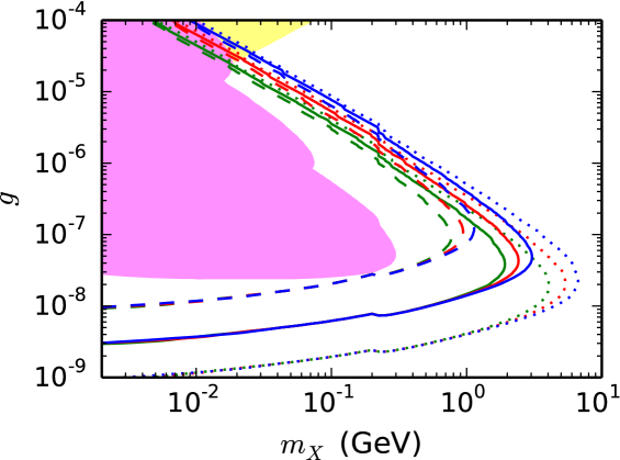
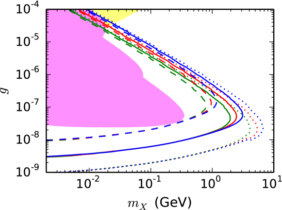
Figure 1: Contours of expected number of signal events for the $U(1)_{e-\mu}$ model. The beam energy is taken to be $E_{\rm beam}=125$ (green), $250$ (red), and $500\,{\rm GeV}$ (blue). The dotted, solid, and dashed lines are for $N_{\rm sig}=10^{-2}$, $1$, and $10^{2}$, respectively, taking $N_{e}=4\times 10^{21}$. The mixing parameter is taken to be $\kappa_{\epsilon}=1$. The pink and yellow shaded regions are excluded by beam dump and neutrino-electron scattering experiments, respectively.

Figure 2: Same as Fig. 2, but for the $U(1)_{e-\tau}$ model.

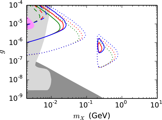
Figure 3: Contours of expected number of signal events for the $U(1)_{e-\tau}$ model. The beam energy is taken to be $E_{\rm beam}=125$ (green), $250$ (red), and $500\,{\rm GeV}$ (blue). The dotted, solid, and dashed lines are for $N_{\rm sig}=10^{-2}$, $1$, and $10^{2}$, respectively, taking $N_{e}=4\times 10^{21}$. The mixing parameter is taken to be $\kappa_{\epsilon}=1$. The pink region is excluded by beam dump experiment. The light- and dark-gray regions show the constraint from the BBN and SN1987A, respectively.

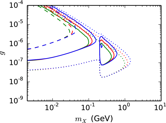
Figure 4: Same as Fig. 2, but for the $U(1)_{\mu-\tau}$ model with $\kappa_{\epsilon}=5$.

Next, we consider the case of the $U(1)_{\mu-\tau}$ model; in Fig. 3, the expected number of signal events is shown, taking $\kappa_{\epsilon}=1$. The constraints from the beam dump experiment [34], big bang nucleosynthesis (BBN) [27], and SN1987A [35] are shown in the pink, light gray, and dark gray shaded regions, respectively. We can see that the ILC beam dump experiment may access the parameter region which has not been excluded yet. In particular, the region with $(m_{X},g)\sim(10\,{\rm MeV},10^{-5})$ may be covered; such a parameter region is interesting because the Hubble tension may be alleviated [27]. As one can see, compared to the cases of the $U(1)_{e-\mu}$ and $U(1)_{e-\tau}$ models, the expected number of the signal events is significantly suppressed. This is because, in the $U(1)_{\mu-\tau}$ model, the LGB does not directly couples to the electron (or positron) which is the incident particle to cause the LGB production. The LGB production is via the LGB-photon mixing and hence is significantly suppressed because $e_{\rm EM}|\epsilon_{\rm eff}|\ll g$. We can also see that $N_{\rm sig}$ is enhanced when $m_{X}>2m_{\mu}$. This is due to the fact that, in the $U(1)_{\mu-\tau}$ model, the LGB directly couples to $\mu^{\pm}$ and hence Br$(X\rightarrow\mu^{+}\mu^{-})$ is sizable if the process is kinematically allowed. Thus, when $m_{X}>2m_{\mu}$, we can use $\mu^{+}\mu^{-}$ final state for the LGB search while, for $m_{X}<2m_{\mu}$, we can only use $X\rightarrow e^{+}e^{-}$ final state whose branching fraction is very small in the $U(1)_{\mu-\tau}$ model.

Because the production of the LGB is though the LGB-photon mixing in the $U(1)_{\mu-\tau}$ model, the production cross section of the LGB is sensitive to the tree-level mixing parameter $\epsilon_{0}$ (and hence to $\epsilon_{\rm eff}$). In addition, the mixing is important for the decay process $X\rightarrow e^{+}e^{-}$ which only provides the visible final state when $m_{X}<2m_{\mu}$. Consequently, $N_{\rm sig}$ is highly dependent on $\epsilon_{\rm eff}$. In particular, if $\epsilon_{\rm eff}$ is enhanced, the ILC beam dump experiment has a higher sensitivity to the parameter space (i.e., $m_{X}$ vs. $g$ plane) of the $U(1)_{\mu-\tau}$ model. To see this, In Fig. 4, we show the contours of constant $N_{\rm sig}$, taking $\kappa_{\epsilon}=5$. We can see that, for fixed values of $m_{X}$ and $g$, the expected number of the signal events is enhanced with the increase of $\kappa_{\epsilon}$.

4 Discrimination of Models

Even though a signal of the LGB production can be found at the ILC beam dump experiment, it is unclear how and how well the properties of the newly found particle (i.e., in the present case, the LGB) can be studied after the discovery. In this section, we consider the situation after the discovery of the LGB at the ILC beam dump experiment and discuss whether we may understand its properties.

The information about the LGB mass is embedded in the momentum information of the final state particles. In particular, the LGB may decay into $e^{+}e^{-}$ and/or $\mu^{+}\mu^{-}$ pair. Thus, if the momenta (or the energy) of the visible final state particles are measured with a reasonable accuracy, the mass of the LGB can be determined.

With identifying the final state particles from the decay, information about the decay modes of $X$ can be also obtained. Such a study is of interest in particular when $m_{X}\gtrsim 2m_{\mu}$ because the possible final states as well as the branching ratios to those final states are strongly dependent on the model. If $m_{X}<2m_{\mu}$, on the contrary, visible decay mode is only $X\rightarrow e^{+}e^{-}$ irrespective of the model. For such a light LGB, its properties are hardly clarified by the study of the decay modes. Hereafter, we assume that, after the observations of the signals, the mass of $X$ is determined with some accuracy and is found to be $2m_{\mu}<m_{X}<2m_{\tau}$. (As shown in the previous section, the ILC beam dump experiment may not have a good sensitivity to LGBs heavier than $\sim 2m_{\tau}$.)

In the following, we discuss the discrimination of the models based on the decay modes of $X$. We pay attention to the early stage of the discovery at which $\sim 10$ signal events are available to study the properties of the LGB. In order to estimate how well we can determine the decay properties of the LGB, we consider a simple analysis using the following quantities:

$$r_{e}\equiv \,\frac{\Gamma(X\rightarrow e^{+}e^{-})}{\Gamma_{X}^{({\rm vis})}},$$ (4.1)

$$r_{\mu}\equiv \,\frac{\Gamma(X\rightarrow\mu^{+}\mu^{-})}{\Gamma_{X}^{({\rm vis})}},$$ (4.2)

$$r_{h}\equiv \,\frac{\Gamma(X\rightarrow{\rm hadrons})}{\Gamma_{X}^{({\rm vis})}},$$ (4.3)

where $\Gamma_{X}^{({\rm vis})}$ is the partial width with visible final states. In the case of $m_{X}<2m_{\tau}$, $\Gamma_{X}^{({\rm vis})}$ becomes the following:

$$\Gamma_{X}^{({\rm vis})}\equiv\Gamma(X\rightarrow e^{+}e^{-})+\Gamma(X\rightarrow\mu^{+}\mu^{-})+\Gamma(X\rightarrow{\rm hadrons}).$$ (4.4)

We consider the case of $m_{X}<2m_{\tau}$ so that $r_{e}+r_{\mu}+r_{h}=1$. For the case of the LGB of the $U(1)_{e-\mu}$ gauge symmetry,

$$r_{e}^{(e-\mu)}\simeq r_{\mu}^{(e-\mu)}\simeq 0.5,~{}~{}~{}r_{h}^{(e-\mu)}\simeq 0,$$ (4.5)

while for $U(1)_{e-\tau}$,

$$r_{e}^{(e-\tau)}\simeq 1.0,~{}~{}~{}r_{\mu}^{(e-\tau)}\simeq r_{h}^{(e-\tau)}\simeq 0.$$ (4.6)

Notice that one interesting question is whether the LGBs may be distinguished from the dark photon (denoted as $\gamma^{\prime}$) which universally couples to all the charged particles via the kinetic mixing with the electromagnetic photon. For the case of dark photon (with $m_{\mu}\ll m_{\gamma^{\prime}}\ll m_{\tau}$), we find

$$r_{e}^{(\gamma^{\prime})}\simeq r_{\mu}^{(\gamma^{\prime})}\simeq\frac{1}{2+R}\ ,~{}~{}~{}r_{h}^{(\gamma^{\prime})}\simeq\frac{R}{2+R}\ ,$$ (4.7)

where $R$ is the $R$-ratio for $q^{2}=m_{\gamma^{\prime}}^{2}$, with $m_{\gamma^{\prime}}$ being the mass of the dark photon. This may help to distinguish the LGBs and the dark photon because the LGBs dominantly decay into leptonic final states.

In order to study how well various models can be distinguished after the discovery of the signal events, we assume a situation in which the signal events with $e^{+}e^{-}$, $\mu^{+}\mu^{-}$, and hadronic final states are observed with the event numbers of $n_{e}^{\rm(obs)}$, $n_{\mu}^{\rm(obs)}$, and $n_{h}^{\rm(obs)}$, respectively. Then, treating $r_{e}$ and $r_{\mu}$, as well as the total number of signal events, as model parameters, we adopt the following likelihood function on the $r_{e}$ vs. $r_{\mu}$ plane:

$$\mathcal{L}(r_{e},r_{\mu},r_{h};n_{e}^{\rm(obs)},n_{\mu}^{\rm(obs)},n_{h}^{\rm(obs)})=\mathcal{N}\mathcal{P}(r_{e}n_{\rm tot};n_{e}^{\rm(obs)})\mathcal{P}(r_{\mu}n_{\rm tot};n_{\mu}^{\rm(obs)})\mathcal{P}(r_{h}n_{\rm tot};n_{h}^{\rm(obs)}),$$ (4.8)

where $r_{h}=1-r_{e}-r_{\mu}$, $\mathcal{N}$ is the normalization factor, $n_{\rm tot}\equiv n_{e}^{\rm(obs)}+n_{\mu}^{\rm(obs)}+n_{h}^{\rm(obs)}$, and $\mathcal{P}(n,n^{\rm(obs)})\equiv n^{n^{\rm(obs)}}e^{-n}/n^{\rm(obs)}!$ is the Poisson distribution function. The normalization factor $\mathcal{N}$ is determined so that

$$\int_{0}^{1}dr_{e}\int_{0}^{1-r_{e}}dr_{\mu}\mathcal{L}(r_{e},r_{\mu},r_{h};n_{e}^{\rm(obs)},n_{\mu}^{\rm(obs)},n_{h}^{\rm(obs)})=1.$$ (4.9)

Using the above likelihood function, we determine the allowed regions with given confidence levels.

First, we consider the $U(1)_{e-\mu}$ LGB. In Figs. 6 and 6, the expected constraint on $r_{e}$, $r_{\mu}$ and $r_{h}$ are given on the ternary plot, taking $(n_{e}^{\rm(obs)},n_{\mu}^{\rm(obs)},n_{h}^{\rm(obs)})=(5,5,0)$ and $(10,10,0)$, respectively. With the discovery of $\sim 10$ – $20$ signals of the $U(1)_{e-\mu}$ LGB, we may discriminate the possibility of the $U(1)_{e-\tau}$ model which predicts $(r_{e},r_{\mu},r_{h})\simeq(1,0,0)$. On the figures, we also show the prediction of the dark photon, which is given as a line because the prediction of the dark photon depends on the $R$-ratio. For the case of the dark photon, $r_{h}^{(\gamma^{\prime})}$ can take any value between $0$ and $\sim 1$ because $R$ varies from $\sim 0$ to $\sim 50$ [36]; the predictions for the cases of $m_{\gamma^{\prime}}=400$, $450$, $500$, $550$, and $600\,{\rm MeV}$ are also plotted. For the case of the $U(1)_{e-\mu}$ model, the parameter region of the dark photon model with $r_{h}^{(\gamma^{\prime})}\sim 0$ is hardly excluded solely by the study of the decay mode; if information about the mass of the LGB becomes available, the dark photon model may be excluded. For example, $r_{h}^{(\gamma^{\prime})}\gtrsim 0.3$ if $m_{\gamma^{\prime}}\gtrsim 550\,{\rm MeV}$. Thus, if $m_{X}$ is found to be heavier than $\sim 550\,{\rm MeV}$, we may exclude the possibility of the dark photon with accumulating $\sim 20$ signal events from the decay of the $U(1)_{e-\mu}$ LGB.

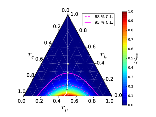
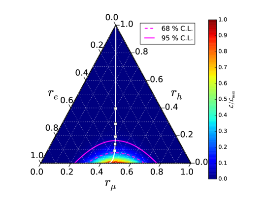
Figure 5: Expected constraint on $r_{e}$, $r_{\mu}$, and $r_{h}$ parameters in the $U(1)_{e-\mu}$ model for $(n_{e}^{\rm(obs)},n_{\mu}^{\rm(obs)},n_{h}^{\rm(obs)})=(5,5,0)$. The magenta lines are expected constraint at $68\,\%$ (dashed) and $95\,\%$ (solid) C.L. The white line shows the prediction of the dark photon model; squares on the white line are the predictions for the cases of $m_{\gamma^{\prime}}=400$, $450$, $500$, $550$, and $600\,{\rm MeV}$ from below. The background color indicates the ratio $\mathcal{L}/\mathcal{L}_{\rm max}$, where $\mathcal{L}_{\rm max}$ is the maximal value of the likelihood.

Figure 6: Same as Fig. 6, but for $(n_{e}^{\rm(obs)},n_{\mu}^{\rm(obs)},n_{h}^{\rm(obs)})=(10,10,0)$.

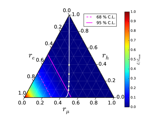
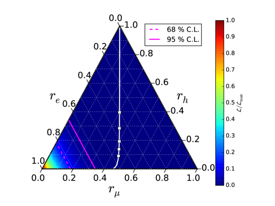
Figure 7: Same as Fig. 6, but for the $U(1)_{e-\tau}$ model taking $(n_{e}^{\rm(obs)},n_{\mu}^{\rm(obs)},n_{h}^{\rm(obs)})=(5,0,0)$.

Figure 8: Same as Fig. 6, but for the $U(1)_{e-\tau}$ model taking $(n_{e}^{\rm(obs)},n_{\mu}^{\rm(obs)},n_{h}^{\rm(obs)})=(10,0,0)$.

For the case of the $U(1)_{e-\tau}$ model, the LGB dominantly decays into the $e^{+}e^{-}$ final state (as well as into the neutrino pair); the effect of the mixing is negligibly small when the number of signal events is $\sim 10$. In Figs. 8 and 8, we show the expected constraint on $r_{e}$, $r_{\mu}$ and $r_{h}$ parameters, taking $(n_{e}^{\rm(obs)},n_{\mu}^{\rm(obs)},n_{h}^{\rm(obs)})=(5,0,0)$ and $(10,0,0)$, respectively. We can see that the LGB of the $U(1)_{e-\tau}$ model can be distinguished from that of the $U(1)_{e-\mu}$ model and the dark photon if more than $\sim 5$ signal events are observed, assuming that the mass of the LGB is measured to be heavier than $\sim 2m_{\mu}$.

So far, we did not consider using the number of signal events $N_{\rm sig}$ for the study of the LGB properties. As indicated by the figures, $N_{\rm sig}$ is sensitive to the mass and the coupling constants so that the measurement of the event rate may provide information about the mass and the coupling constant of the LGB. In particular, the event rate may be sizable in the $U(1)_{e-\mu}$ and $U(1)_{e-\tau}$ models even if the LGB mass is relatively large, while it is relatively suppressed in the $U(1)_{\mu-\tau}$ model even if the LGB mass is small. Thus, combining with the kinematical determination of the LGB mass, we may distinguish the $U(1)_{\mu-\tau}$ model from others using the event rate information. We should, however, note that the production cross section of the LGB, as well as the efficiency of the signal detection, should be well understood for the study using the event rate; such a study is beyond the scope of our analysis and we leave it as a future task.

5 Conclusions and Discussion

In this paper, we have considered the possibility to search for the LGBs, i.e., gauge bosons in association with $U(1)_{e-\mu}$, $U(1)_{e-\tau}$, and $U(1)_{\mu-\tau}$ gauge symmetries, at the ILC beam dump experiment. Installing shields, vetos, and decay volume with detectors, the ILC beam dump experiment is capable of detecting the signals of the LGBs with very small couplings which are hardly studied by the conventional ILC setup only with the detector for the energetic $e^{+}e^{-}$ collision. Assuming that the LGBs are light and weakly interacting, we have calculated the expected number of events and confirmed that a significant number of LGB signals may be possible. We have seen that the ILC beam dump experiment can cover the parameter regions which have not been explored before. Such a study may open a new window to BSM physics.

In our calculation, we have concentrated on the production process $e^{\pm}N\rightarrow e^{\pm}XN^{\prime}$, which exists irrespective of the species of the injected beam and the detailed setup of the shield. In fact, there may exist other production processes of the LGBs for a particular setup. For example, if a thick lead is adopted as the muon shield, the high intensity muons produced at the dump may also play the role of the initial-state particle to produce the LGBs [11]. Such a possibility may be of interest particularly for the case of $U(1)_{\mu-\tau}$ model for which the ILC beam dump experiment has less sensitivity than the $U(1)_{e-\mu}$ and $U(1)_{e-\tau}$ models if we just consider the production process of $e^{\pm}N\rightarrow e^{\pm}XN^{\prime}$. In addition, if the positron is used as the initial-state particle injected into the dump, the pair annihilation process $e^{+}e^{-}\rightarrow X$ (with $e^{-}$ being the electron in ${\rm H_{2}O}$) may also contribute to the production process [39]. These production processes require particular setups of the experiment, and have not been studied in our analysis; the effects of these processes on the search of the LGBs will be discussed elsewhere [40].

Acknowledgments: This work was supported by JSPS KAKENHI Grant Numbers JP19J13812 (KA), 16H06490 (TM), and 18K03608 (TM). All the ternary plots are generated with python-ternary [41].

References

- [1] T. Behnke et al., eds., The International Linear Collider Technical Design Report - Volume 1: Executive Summary, 1306.6327.
- [2] H. Baer et al., eds., The International Linear Collider Technical Design Report - Volume 2: Physics, 1306.6352.
- [3] C. Adolphsen et al., eds., The International Linear Collider Technical Design Report - Volume 3.I: Accelerator & in the Technical Design Phase, 1306.6353.
- [4] C. Adolphsen et al., eds., The International Linear Collider Technical Design Report - Volume 3.II: Accelerator Baseline Design, 1306.6328.
- [5] H. Abramowicz et al., The International Linear Collider Technical Design Report - Volume 4: Detectors, 1306.6329.
- [6] S. Kanemura, T. Moroi and T. Tanabe, Beam dump experiment at future electron–positron colliders, Phys. Lett. B 751 (2015) 25 [1507.02809].
- [7] B. Holdom, Two U(1)’s and Epsilon Charge Shifts, Phys. Lett. B 166 (1986) 196.
- [8] J. Jaeckel and A. Ringwald, The Low-Energy Frontier of Particle Physics, Ann. Rev. Nucl. Part. Sci. 60 (2010) 405 [1002.0329].
- [9] A. Ringwald, Exploring the Role of Axions and Other WISPs in the Dark Universe, Phys. Dark Univ. 1 (2012) 116 [1210.5081].
- [10] A. Ringwald, Searching for axions and ALPs from string theory, J. Phys. Conf. Ser. 485 (2014) 012013 [1209.2299].
- [11] Y. Sakaki and D. Ueda, Searching for new light particles at the international linear collider main beam dump, Phys. Rev. D 103 (2021) 035024 [2009.13790].
- [12] R. Foot, New Physics From Electric Charge Quantization?, Mod. Phys. Lett. A 6 (1991) 527.
- [13] X.G. He, G.C. Joshi, H. Lew and R.R. Volkas, NEW Z-prime PHENOMENOLOGY, Phys. Rev. D 43 (1991) 22.
- [14] X.-G. He, G.C. Joshi, H. Lew and R.R. Volkas, Simplest Z-prime model, Phys. Rev. D 44 (1991) 2118.
- [15] R. Foot, X.G. He, H. Lew and R.R. Volkas, Model for a light Z-prime boson, Phys. Rev. D 50 (1994) 4571 [hep-ph/9401250].
- [16] N.F. Bell and R.R. Volkas, Bottom up model for maximal muon-neutrino - tau-neutrino mixing, Phys. Rev. D 63 (2001) 013006 [hep-ph/0008177].
- [17] A.S. Joshipura and S. Mohanty, Constraints on flavor dependent long range forces from atmospheric neutrino observations at super-Kamiokande, Phys. Lett. B 584 (2004) 103 [hep-ph/0310210].
- [18] A. Bandyopadhyay, A. Dighe and A.S. Joshipura, Constraints on flavor-dependent long range forces from solar neutrinos and KamLAND, Phys. Rev. D 75 (2007) 093005 [hep-ph/0610263].
- [19] A. Samanta, Long-range Forces : Atmospheric Neutrino Oscillation at a magnetized Detector, JCAP 09 (2011) 010 [1001.5344].
- [20] T. Araki, J. Heeck and J. Kubo, Vanishing Minors in the Neutrino Mass Matrix from Abelian Gauge Symmetries, JHEP 07 (2012) 083 [1203.4951].
- [21] J. Heeck, Neutrinos and Abelian Gauge Symmetries, Ph.D. thesis, Heidelberg U., 2014.
- [22] K. Asai, K. Hamaguchi and N. Nagata, Predictions for the neutrino parameters in the minimal gauged U(1) model, Eur. Phys. J. C 77 (2017) 763 [1705.00419].
- [23] K. Asai, K. Hamaguchi, N. Nagata, S.-Y. Tseng and K. Tsumura, Minimal Gauged U(1) Models Driven into a Corner, Phys. Rev. D 99 (2019) 055029 [1811.07571].
- [24] K. Asai, Predictions for the neutrino parameters in the minimal model extended by linear combination of U(1), U(1) and U(1)B-L gauge symmetries, Eur. Phys. J. C 80 (2020) 76 [1907.04042].
- [25] E. Ma and D.P. Roy, Anomalous neutrino interaction, muon g-2, and atomic parity nonconservation, Phys. Rev. D 65 (2002) 075021 [hep-ph/0111385].
- [26] S. Baek, N.G. Deshpande, X.G. He and P. Ko, Muon anomalous g-2 and gauged L(muon) - L(tau) models, Phys. Rev. D 64 (2001) 055006 [hep-ph/0104141].
- [27] M. Escudero, D. Hooper, G. Krnjaic and M. Pierre, Cosmology with A Very Light Lμ Lτ Gauge Boson, JHEP 03 (2019) 071 [1901.02010].
- [28] T. Araki, K. Asai, K. Honda, R. Kasuya, J. Sato, T. Shimomura et al., Resolving the Hubble tension in a U(1) model with Majoron, 2103.07167.
- [29] Y.-S. Tsai, Axion Bremsstrahlung by an Electron Beam, Phys. Rev. D 34 (1986) 1326.
- [30] K.J. Kim and Y.-S. Tsai, Improved Weizsacker-Williams Method and Its Application to Lepton and W Boson Pair Production, Phys. Rev. D 8 (1973) 3109.
- [31] J.D. Bjorken, R. Essig, P. Schuster and N. Toro, New Fixed-Target Experiments to Search for Dark Gauge Forces, Phys. Rev. D 80 (2009) 075018 [0906.0580].
- [32] S. Andreas, C. Niebuhr and A. Ringwald, New Limits on Hidden Photons from Past Electron Beam Dumps, Phys. Rev. D 86 (2012) 095019 [1209.6083].
- [33] SHiP collaboration, A facility to Search for Hidden Particles (SHiP) at the CERN SPS, 1504.04956.
- [34] M. Bauer, P. Foldenauer and J. Jaeckel, Hunting All the Hidden Photons, JHEP 07 (2018) 094 [1803.05466].
- [35] D. Croon, G. Elor, R.K. Leane and S.D. McDermott, Supernova Muons: New Constraints on ’ Bosons, Axions and ALPs, JHEP 01 (2021) 107 [2006.13942].
- [36] Particle Data Group collaboration, Review of Particle Physics, PTEP 2020 (2020) 083C01.
- [37] T. Araki, S. Hoshino, T. Ota, J. Sato and T. Shimomura, Detecting the gauge boson at Belle II, Phys. Rev. D 95 (2017) 055006 [1702.01497].
- [38] Y. Jho, Y. Kwon, S.C. Park and P.-Y. Tseng, Search for muon-philic new light gauge boson at Belle II, JHEP 10 (2019) 168 [1904.13053].
- [39] Y. Sakaki, Talk given at LCWS2021, https://indico.cern.ch/event/995633/contributions/4256388.
- [40] K. Asai, T. Moroi and A. Niki, Work in progress.
- [41] M. Harper et al., python-ternary: Ternary plots in python, Zenodo 10.5281/zenodo.594435 .