S2R-DepthNet: Learning a Generalizable Depth-specific Structural Representation

Abstract

Human can infer the 3D geometry of a scene from a sketch instead of a realistic image, which indicates that the spatial structure plays a fundamental role in understanding the depth of scenes. We are the first to explore the learning of a depth-specific structural representation, which captures the essential feature for depth estimation and ignores irrelevant style information. Our S2R-DepthNet (Synthetic to Real DepthNet) can be well generalized to unseen real-world data directly even though it is only trained on synthetic data. S2R-DepthNet consists of: a) a Structure Extraction (STE) module which extracts a domain-invariant structural representation from an image by disentangling the image into domain-invariant structure and domain-specific style components, b) a Depth-specific Attention (DSA) module, which learns task-specific knowledge to suppress depth-irrelevant structures for better depth estimation and generalization, and c) a depth prediction module (DP) to predict depth from the depth-specific representation. Without access of any real-world images, our method even outperforms the state-of-the-art unsupervised domain adaptation methods which use real-world images of the target domain for training. In addition, when using a small amount of labeled real-world data, we achieve the state-of-the-art performance under the semi-supervised setting. The code and trained models are available at https://github.com/microsoft/S2R-DepthNet.

1 Introduction

Monocular depth estimation is a long-standing challenging task, which aims to predict the continuous depth value of each pixel from a single color image. This task has a wide range of application in various fields, such as autonomous driving [11, 14], 3D scene reconstruction [49, 21] and robot navigation [44], etc. Recently, a wide variety of algorithms based on deep convolutional neural networks (DCNNs) have achieved good performance with sufficient amounts of annotated data [17, 3, 46, 8, 27, 7, 6]. However, obtaining depth annotations is costly and time-consuming [11, 14, 1]. Some recent methods have investigated self-supervised depth estimation from stereo images pairs [11, 14] or video sequence  [58, 15, 56] by view reconstruction. But stereo pairs or video sequences may not always be available in existing datasets. Besides, these models are often limited to the training dataset domain, having difficulty in scaling to various application scenes.

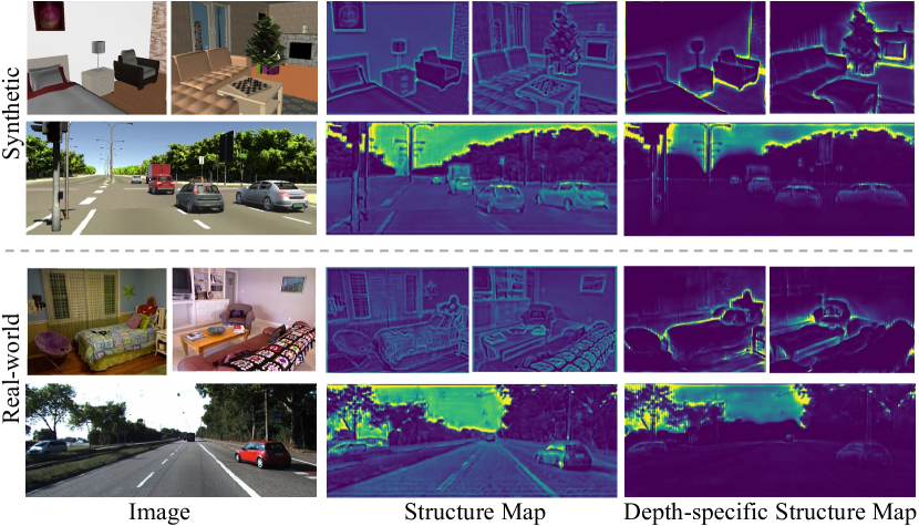
Figure 1: Visualization of our learnt structural representations. It can be seen that even though the input color images from synthetic dataset and real-world dataset are very different in appearance, our structural representations share many similarities, such as layout and object shapes, etc. Furthermore, our depth-specific structure map suppresses the depth-irrelevant structures on the smooth surface, e.g., lanes on the road and photos on the wall.

Some researchers switched to use synthetic images [9, 40] for training where depth annotations can be acquired directly. However, there is usually a domain gap between synthetic data and real-world data, which is caused by style discrepancies across different domains. To address this issue, some domain adaptation methods [55, 1, 25, 53] try to align the feature space of synthetic and real-world images [55, 25] or translate synthetic images to realistic-looking ones [55, 1, 53]. However, these methods all require access to the real-world images of the target domain during the training process, but it is impractical to collect real-world images of various scenes.

Given the above limitations, we consider a more practical domain generalization scenario. In our setting, we only use a large amount of labeled synthetic data without access of any real-world images of the target domain in the training stage. Compared to domain adaptation methods, this is a more difficult task, because we do not even know the style of the real-world images during the training process.

Aiming for better generalizable depth estimation, we need to seek for the essential representation for this task. Structure information is found to be very important for this task  [18, 53, 60, 3, 35], and some previous works explore introducing heuristic structure information to network architecture [3, 35] or loss design [53, 18, 60, 35]. We are the first one to explore learning a depth-specific structural representation for generalizable depth estimation. The image representation can be decomposed into a domain-invariant structure component and a domain-specific style component [24, 19, 20]. The structure component can be further divided into a depth-specific structure component and a depth-irrelevant structure component. The depth-specific structure component is the most essential for depth estimation and can be effectively transferred from synthetic domain to real-world domain.

In order to obtain the depth-specific structural representation, we first extract a general domain-invariant structure map from the image using a proposed Structure Extraction (STE) module by decomposing the image into structure and style components inspired by  [20]. However, the structural representation we thus obtain is a general and low-level image structure, which contains a large amount of depth-irrelevant structures, such as structures on a smooth surface (e.g. lanes on the road or photos on the wall). Furthermore, we propose a Depth-specific Attention (DSA) module to extract high-level semantic information from the input image and help to suppress the depth-irrelevant structures. Since only depth-specific structural information can pass the STE and DSA modules to the depth prediction (DP) module, our S2R-DepthNet trained on synthetic data can be well generalized to unseen real-world images.

We visualise our learnt structural representation and depth-specific structural representation in Figure 1. Even though there is a distinct style difference between the images from synthetic and real-world image dataset, our learnt structure maps and depth-specific structure maps share many similarities. Furthermore, the depth-specific structure map discards depth-irrelevant structures, e.g. lanes. The highlighted sky is an important cue for vanishing point that is helpful for depth estimation, which is similar to [18].

Main contributions: $(i)$ We are the first to learn a structural representation for generalizable depth estimation, which captures essential structural information and discards style information. S2R-DepthNet can be well generalized to unseen real-world data when only trained on synthetic data. $(ii)$ We propose a two-stage structural representation learning pipeline: a general low-level Structure Extraction module to discard style information and a Depth-specific Attention module to suppress depth-irrelevant structure with depth-specific knowledge. $(iii)$ We enable a more practical scenario for the depth estimation task, where there is only a large amount of synthetic data but it is hard to acquire real-world data images or depth annotations.

We carry out extensive experiments to demonstrate the effectiveness of our proposed domain-invariant structural representations. Even though we do not use real-world images for training, our method still outperforms the state-of-the-art domain adaptation methods that use real-world images of the target domain for training. Surprisingly, when our method uses a small amount of labeled real-world data for training, it also achieves the state-of-the-art performance under the semi-supervised setting.

2 Related Work

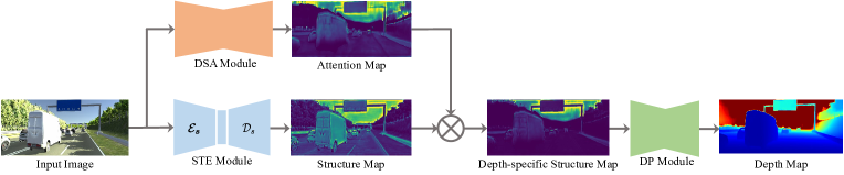
Figure 2: An overview of S2R-DepthNet. Our overall architecture consists of a Structure Extraction (STE) module which extracts a domain-invariant structure map, a Depth-specific Attention (DSA) module which suppresses depth-irrelevant structures by predicting an attention map, and a Depth Prediction (DP) module to predict the final depth map from depth-specific structural representation. $\otimes$ denotes element-wise multiplication.

Monocular Depth Estimation.

The monocular depth estimation task aims to estimate depth from a single image. Previous works explore the network structure [17, 27, 8, 47, 3, 45] or are jointly trained with other tasks, e.g., normal [34, 50], optical flow [51, 4] and segmentation [16, 42]. All these works are trained and tested on datasets of a specific domain without considering domain gaps. It is easy for the method to overfit the specific training dataset and lose the capability of generalization. However, obtaining various depth annotations is costly and time-consuming. Some self-supervised methods [15, 57, 43, 51] take video sequences or stereo pairs as training data and use image warping and reconstruction loss to replace explicit depth supervision. However, dynamic objects and low-texture regions are still a challenge for these methods. Our work is the first one to explore another promising direction, which uses only synthetic data for training and tests directly on real data.

Domain Adaptation and Generalization.

The domain adaptation [10, 30, 36] and generalization [31, 37] methods deal with the domain gap between the training and testing datasets. Domain adaptation methods transfer the model trained on the source domain by seeing data in the target domain while domain generalization only performs training on the source domain and tests on the unseen domain. Inspired by the domain adaptation works, researchers try to leverage synthetic data for training a depth estimation model and transfer it to real data. These works can be roughly divided into two categories: aligning the feature space of synthetic and real images [55, 25, 1] and translating synthetic images to realistic-looking ones [55, 1, 53]. Those methods all need access to real images of the target domain, which means it is still necessary to collect real images for training. Our method gets rid of this limitation since we do not use any real images for training and it holds the potential for wider applications.

Image Translation and Style Transfer.

The image translation task translates images from one domain to another [20, 12, 22]. The previous works [24, 19, 20] decompose image representation into a domain-invariant structure component and a domain-specific style component. Specifically, Kazemi et al.[24] present the style and structure disentangled GAN that learns to disentangle style and structure representations for image generation. Huang et al.[20] disentangle image representation into structure and style codes, and recombine its structure code with a random style code sampled from the style space of the target domain to translate an image to another domain. Targeting for translating images from one style to another, those works extract a structural representation which is disentangled from domain styles. Our goal is to seek for the essential generalizable structural representation for the depth estimation task by getting rid of the influence of irrelevant factors.

3 Depth-specific Structural Learning

In this section, we first present an overview of our S2R-DepthNet, then introduce its key modules, and finally provide the training procedure.

3.1 S2R-DepthNet

Our S2R-DepthNet is a generalizable depth prediction framework based on depth-specific structural representation leaning. As shown in Figure 2, our framework consists of Structure Extraction (STE) module $\mathcal{S}$, Depth-specific Attention (DSA) module $\mathcal{A}$ and a Depth Prediction (DP) module $\mathcal{P}$. To capture the essential representation for depth estimation, we design a two-stage learning pipeline: the STE module to extract a domain-invariant structural representation $M_{s}$ by disentangling the image into structure and style components, and the DSA module to suppress depth-irrelevant structure with task-specific attention $M_{a}$, resulting in a depth-specific structure map $M_{sa}$. Finally, we feed $M_{sa}$ into the DP module $\mathcal{P}$ to predict the depth.

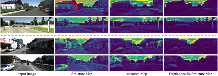
Figure 3: Visualization of intermediate results. The top and bottom two rows are respectively the generated results for synthetic images and real-world images by our S2R-DepthNet trained on synthetic images.

3.2 Structure Extraction Module

The STE module aims to extract domain-invariant structure information from images with different styles. The STE module consists of an encoder $\mathcal{E}_{s}$ to extract structure information and a decoder $\mathcal{D}_{s}$ to decode the encoded structure information into a structure map as shown in Figure 2.

Inspired by the image translation work [20], we adopt an image translation framework to train the encoder $\mathcal{E}_{s}$. In order to make the $\mathcal{E}_{s}$ generalizable to various style images, we choose the Painter By Numbers (PBN) dataset with a large style variation as the target domain for image translation and the images of a synthetic dataset as the source domain. We use a shared $\mathcal{E}_{s}$ to extract structure for both the source and target datasets. This is different from [20] which uses different encoders for the source and target datasets. Thus $\mathcal{E}_{s}$ can see various styles of data and extract structural features that are not sensitive to any specific style. After the training of $\mathcal{E}_{s}$, we can extract the structure information from the synthetic images. The weights of $\mathcal{E}_{s}$ are fixed when training other modules to maintain its ability for general structure extraction.

In order to restore the spatial structure of the encoded information of $\mathcal{E}_{s}$, we choose to use a decoder $\mathcal{D}_{s}$ to reconstruct a structure map $M_{s}$ with the same spatial resolution as the input image. Since there is no ground truth of this structure map, we feed the structure map to the DP module, and use the ground truth depth to train $\mathcal{D}_{s}$. We add a heuristic regularization loss to the structure map by encouraging the value of the structure map to be small wherever the depth map is smooth. Given the input image $I$ and corresponding ground truth $D$, the loss for training $\mathcal{D}_{s}$ is

$$\mathcal{L}_{\mathcal{S}} =\sum_{p}||\hat{D}(p)-D(p)||_{1}+$$

$$\lambda\sum_{p}||M_{s}(p)||_{1}\cdot e^{-\beta(|\nabla_{x}D(p)+\nabla_{y}D(p)|)},$$ (1)

where $\hat{D}$ is the predicted depth map , $p$ is the index of pixels, $\nabla_{x}$ and $\nabla_{y}$ are horizontal and vertical gradient operators respectively, $\lambda$ and $\beta$ are the hyper parameters.

3.3 Depth-specific Attention Module

Our goal is to learn essential structural representation for generalizable depth estimation. Currently the structure map from the STE module contains abundant low level structures including a large amount of depth-irrelevant structures, such as detailed texture structures on smooth surfaces. The encoder of the STE module is designed to capture low-level features with only 4 times downsampling. Besides, there are a lot of Instance Normalization (IN) operations in the encoder for better generalization, which leads to the loss of discriminative features [19, 32, 23] and is harmful for semantic feature extraction. In contrast, many researchers have found that high-level semantic knowledge [41, 18, 17, 3] is important for the depth estimation task.

To extract more influential high-level semantic knowledge for depth estimation, we design a DSA module to predict an attention map $A$ from the raw input image. This attention map helps to suppress depth-irrelevant structures by leveraging high-level semantic information extracted from the raw images. We construct the encoder part of the DSA module using the dilated residual network [52], which utilizes dilated convolutions to increase the receptive field while preserving local detailed information. Then we use a decoder to upsample the encoded features to the original resolution and add a sigmoid layer behind it to generate the attention map. Finally, the obtained attention map is used to weight the general structure map to produce the final depth-specific structure map as:

$$M_{sa}=M_{s}\otimes M_{a},$$ (2)

where $\otimes$ denotes element-wise multiplication.

Since we multiply the attention map and the structure map, extra depth-irrelevant information can hardly pass through this bottleneck and the DP module is forced to estimate depth from this concise and comprehensive depth-specific structure representation.

We fix the parameters of the previously trained STE module, and train the DSA module to suppress depth-irrelevant structures to get the depth-specific structure map. Meanwhile, the DP module is trained to predict depth from the depth-specific structure map. The loss function for training the DSA and DP modules is:

$$\mathcal{L}_{\mathcal{A}} =\sum_{p}||\hat{D}(p)-D(p)||_{1}.$$ (3)

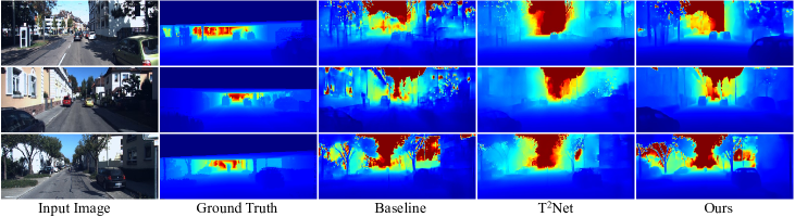
Figure 4: Qualitative comparison of the depth map on the KITTI dataset. The baseline is the DP module only trained on vKITTI dataset. Compared with the approach T²Net[55] and Baseline, our method can restore clear object boundaries, such as cars and trees.

3.4 Training Procedure

In summary, our framework consists of the following modules: STE module $\mathcal{S}$ which consists of its encoder $\mathcal{E}_{s}$ and decoder $\mathcal{D}_{s}$, DSA module $\mathcal{A}$ and DP module $\mathcal{P}$. Instead of training the whole network end-to-end, we design a multi-step training procedure. 1) Train $\mathcal{E}_{s}$ with the synthetic dataset [9] and PBN dataset. The detailed network sturcuture and loss are presented in the supplementary. Then Fix $\mathcal{E}_{s}$ in the following steps. 2) Leave out $\mathcal{A}$, train $\mathcal{D}_{s}$ and $\mathcal{P}$ with the loss defined in Eq. 1 on the synthetic dataset. Fix $\mathcal{D}_{s}$ in the following steps. 3) Involving $\mathcal{A}$, train $\mathcal{A}$ and $\mathcal{P}$ with the loss defined in Eq. 3 on the synthetic dataset. After this training process, we get the whole S2R-DepthNet for tesing real-world images.

4 Experiments

In this section, we first introduce the implementation details and datasets in Section 4.1. We then conduct experiments on synthetic to real-world generalization task for both the outdoor and indoor scenarios. Finally, we provide the ablation studies to analyze the contribution and effectiveness of each module of our framework.

Table 1: Performance on KITTI. All results on KITTI dataset use the Eigen split [7]. K represents KITTI dataset, V is vKITTI dataset, cap means different gt/predicted depth range. For the supervision or not, Yes represents supervised learning, SSL: self-supervised learning, DG: Domain generalization and UDA: the unsupervised domain adaptation. The best results on each metric are marked in bold.

				Higher is better			Lower is better
Method	Dataset	Supervision	cap	$\delta<1.25$	$\delta<1.25^{2}$	$\delta<1.25^{3}$	Abs Rel	Squa Rel	RMSE	RMSElog
Eigen et al.[7]	K	Yes	0$\sim$80m	0.692	0.899	0.967	0.215	1.515	7.156	0.270
Zhou et al.[58]	K (Video)	SSL	0$\sim$80m	0.678	0.885	0.957	0.208	1.768	6.856	0.283
Godard et al.[14]	K (Stereo)	SSL	0$\sim$80m	0.803	0.922	0.964	0.148	1.344	5.927	0.247
DP only (synthetic)	V	DG	0$\sim$80m	0.642	0.861	0.944	0.236	2.171	7.063	0.315
DP only (real-world)	K	Yes	0$\sim$80m	0.804	0.935	0.977	0.141	0.980	5.224	0.217
Kundu et al.[25]	V	UDA	0$\sim$80m	0.665	0.882	0.950	0.214	1.932	7.157	0.295
T2Net [55]	V	UDA	0$\sim$80m	0.757	0.918	0.969	0.171	1.351	5.944	0.247
Ours	V	DG	0$\sim$80m	0.781	0.931	0.972	0.165	1.351	5.695	0.236
Zhou et al.[58]	K (Video)	SSL	0$\sim$50m	0.735	0.915	0.968	0.190	1.436	4.975	0.258
Godard et al.[14]	K (Stereo)	SSL	0$\sim$50m	0.818	0.931	0.969	0.140	0.976	4.471	0.232
DP only (synthetic)	V	DG	0$\sim$50m	0.654	0.872	0.950	0.229	1.726	5.539	0.301
DP only (real-world)	K	Yes	0$\sim$50m	0.819	0.944	0.980	0.136	0.787	3.978	0.205
Kundu et al.[25]	V	UDA	0$\sim$50m	0.687	0.899	0.958	0.203	1.734	6.251	0.284
T2Net [55]	V	UDA	0$\sim$50m	0.773	0.928	0.974	0.164	1.019	4.469	0.231
Ours	V	DG	0$\sim$50m	0.793	0.939	0.976	0.158	1.000	4.321	0.223

4.1 Implementation Details

Network Details.

Our S2R-DepthNet consists of three modules: STE, DSA and DP. STE module is a standard encoder-decoder architecture. The encoder $\mathcal{E}_{s}$ is the same as [20]. The decoder $\mathcal{D}_{s}$ includes two up-projection layers  [27] to restore the encoded structural features to the original image resolution and a convolutional layer to reduce the feature maps into one-channel map. DSA module is also an encoder-decoder structure where we use a dilated residual network [52] as the encoder and three up-projection layers [27] followed by a sigmoid layer as decoder. For DP module, we follow the depth estimation network architecture of previous works [53, 55].

Training Details.

We implement our method based on Pytorch [33]. We follow the same parameters as [20] to train STE module encoder $\mathcal{E}_{s}$. For training the decoder $\mathcal{D}_{s}$ of STE module and joint training DSA module and DP module, we use a step learning rate decay policy with Adam optimizer with an initial learning rate of $10^{-4}$. We reduce the learning rate by 50% every $10$ epochs. We set $\beta_{1}=0.9,\beta_{2}=0.999$, weight decay as $10^{-4}$ and the total number of epochs is $60$. The hyper parmameters $\lambda$ and $\beta$ in Eq. 1 are set to 1 and 0.001, respectively.

Datasets.

For outdoor scenes, we use synthetic Virtual KITTI (vKITTI)  [9] as the source domain dataset. We use the KITTI dataset [13] as the real-world dataset for evaluation. For indoor scenes, we use a synthetic dataset SUNCG as the source domain dataset. We follow  [55] to choose image-depth pairs for training. We use the real-world indoor scene dataset, i.e. NYU Depth v2  [38] for evaluation following the same setting with previous works [55, 25, 17]. We follow the previous work  [7, 8, 27, 58] and use standard evaluation metrics. All results are reported using median scaling as in [25, 58], expect that real-world data is used for semi-supervised training.

Table 2: Performance on KITTI for semi-supervised setting. All results on KITTI dataset use the Eigen split [7]. K represents KITTI dataset,V is vKITTI dataset, cap means different gt/predicted depth range. The best results on each metric are marked in bold.

			Higher is better			Lower is better
Method	Dataset	cap	$\delta<1.25$	$\delta<1.25^{2}$	$\delta<1.25^{3}$	Abs Rel	Squa Rel	RMSE	RMSElog
Kundu et al.[25]	V+K(Small)	0$\sim$80m	0.771	0.922	0.971	0.167	1.257	5.578	0.237
Zhao et al.[54]	V+K(Small)	0$\sim$80m	0.796	0.922	0.968	0.143	0.927	4.694	0.252
Ours-DG	V	0$\sim$80m	0.781	0.931	0.972	0.165	1.351	5.695	0.236
Ours-S	V+K(Small)	0$\sim$80m	0.858	0.955	0.984	0.116	0.766	4.409	0.185
Kuznietsov et al.[26]	K+Stereo	0$\sim$80m	0.862	0.960	0.986	0.113	0.741	4.621	0.189
Kundu et al.[25]	V+K(Small)	0$\sim$50m	0.784	0.930	0.974	0.162	1.041	4.344	0.225
Ours-DG	V	0$\sim$50m	0.793	0.939	0.976	0.158	1.000	4.321	0.223
Ours-S	V+K(Small)	0$\sim$50m	0.870	0.959	0.986	0.111	0.642	3.463	0.176
Kuznietsov et al.[26]	K+Stereo	0$\sim$50m	0.861	0.964	0.989	0.117	0.597	3.531	0.183

4.2 Experimental results

Our settings are similar to the typical unsupervised domain adaptation setting, except that we do not access any real-world images. Therefore, we mainly compare with some state-of-the-art domain adaptation methods on depth estimation [25, 55]. We do not compare with [53] because it is designed for training with real-world stereo pairs. We compare two challenging tasks separately: vKITTI [9] to KITTI [13] and SUNCG [40] to NYU Depth v2 [38]. To better demonstrate the generalizability of our method, we conduct experiments on more auto-driving datasets: Cityscapes [5], DrivingStereo [48] and nuSenses [2]. In addition, when using a small amount of labeled real-world data, we also compare with state-of-the-art methods under the same semi-supervised setting.

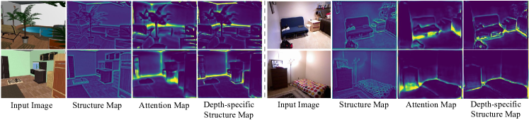
Figure 5: Visualization of the structure maps on SUNCG (left) and NYU Depth v2 (right) datasets. Our depth-specific representations focus on the layout, junctions and object boundaries of indoor scenes.

Table 3: Performance on NYU Depth v2.

Method	Abs Rel	RMSE	$\log{10}$	$\delta<1.25$	$\delta<1.25^{2}$	$\delta<1.25^{3}$
Li et al.[28]	0.232	0.821	0.094	0.621	0.886	0.968
Eigen et al.[7]	0.215	0.907	-	0.611	0.887	0.971
T2Net [55]	0.203	0.738	-	0.670	0.891	0.966
Baseline	0.278	0.899	0.111	0.557	0.826	0.940
+ STE	0.225	0.756	0.093	0.643	0.880	0.962
+ STE + DSA	0.196	0.662	0.082	0.695	0.910	0.972

Table 4: Results on more datasets.

	Higher is better			Lower is better
Settings	$\delta<1.25$	$\delta<1.25^{2}$	$\delta<1.25^{3}$	Abs Rel	Squa Rel	RMSE	RMSElog
Baseline(vKITTI$\to$Cityscapes)	0.516	0.747	0.854	0.297	5.077	13.938	0.452
T2Net(vKITTI$\to$Cityscapes)	0.528	0.760	0.868	0.294	4.639	13.922	0.425
Ours(vKITTI$\to$Cityscapes)	0.663	0.860	0.941	0.208	2.944	11.164	0.314
Baseline(vKITTI$\to$DrivingStereo)	0.408	0.715	0.878	0.374	8.619	15.822	0.440
T2Net(vKITTI$\to$DrivingStereo)	0.546	0.787	0.900	0.302	5.689	12.892	0.377
Ours(vKITTI$\to$DrivingStereo)	0.737	0.917	0.971	0.186	2.710	9.166	0.246
Baseline(vKITTI$\to$nuScenes)	0.543	0.787	0.892	0.289	3.921	11.587	0.406
T2Net(vKITTI$\to$nuScenes)	0.575	0.799	0.895	0.267	3.389	10.809	0.395
Ours(vKITTI$\to$nuScenes)	0.601	0.815	0.908	0.249	2.841	10.200	0.366

vKITTI $\rightarrow$ KITTI.

We report experimental results of the proposed method in Table 1. We use the Eigen split [7] in the KITTI dataset, which is the same as previous methods [7, 29, 58, 14, 25, 55]. The spatial resolutions are also kept the same. We take the DP module trained on vKITTI and tested on KITTI as the baseline denoted as DP only (synthetic). We also provide the result of DP module trained and tested on KITTI for reference (denoted as DP only (real-world)), which can be regarded as the upper bound. We choose previous state-of-the-art unsupervised domain adaptation methods on depth estimation [25, 55] that are most similar to our setting for comparison. We also compare to some supervised and self-supervised methods for reference. However, it is worth noting that even though our method does not use any real-world images for training, it still outperforms the current state-of-the-art unsupervised domain adaptation methods on the depth estimation task. Results from T²Net [55] are recomputed using median scaling with the official pretrained model for fair comparison. Specifically, compared with T²Net [55], our method improves on $\delta<1.25$ by $3.17\%$ at cap of 80m and $2.59\%$ at cap of 50m. The Abs-Rel is reduced by $3.51\%$ at cap of 80m and $3.66\%$ at cap of 50m. RMSE is reduced by $4.19\%$ at cap of 80m and $3.31\%$ at cap of 50m. Even though we do not see the style of real-world images of testing dataset, our proposed method still outperforms the state-of-the-art domain adaptation methods that use real-world image for training. These significant improvements in all the metrics demonstrate that our proposed structural representation has strong generalization capability on unseen scenes.

In order to further verify the effectiveness of our method, we consider another practical scenario in which there is a small amount of real-world ground-truth data available during training [54, 25]. It can be referred to as a semi-supervised setting. For a fair comparison, we follow the previous works [54, 25] and choose the first 1000 ($4.42\%$ of the total dataset) frames in KITTI as the small amount of real-world labeled data used for training. The semi-supervised version of our method is fine-tuned with these 1000 frames of labeled real-world data based on the domain generalization model. The quantitative results are reported in Table 2. Our method achieves the best performance on all the metrics at both 80m and 50m caps compared with previous methods under the same semi-supervised setting [54, 25]. Specifically, compared with Zhao et al.[54], our method reduces Abs-Rel by $18.9\%$, RMSE by $6.1\%$ and improves $\delta<1.25$ by $7.79\%$ at cap of 80m. When compared with Kundu et al.[25], the Abs-Rel is decreased by $31.5\%$, RMSE is decreased by $20.3\%$ and $\delta<1.25$ is increased by $11.0\%$ at cap of 50m. It is worth noting that even though we do not use any real-world data, our domain generalization (DG) version still outperforms Kundu et al.[25]’s semi-supervised version at cap of 80m and 50m. Kuznietsov et al.[26] use the 7346 ($32.5\%$ of total dataset) image-depth pairs and 12600 stereo pairs for training. We still achieve comparable performance with much less real-world data.

As Figure 3 shows, it is obvious that the learned structure maps preserve the fine scene structures. However, these structures contain a lot of depth-irrelevant structures highlighted with red boxes, such as lane lines, textures on houses, etc. The attention maps focus on the object region with geometric structures (such as cars), layout (house silhouette and road guardrail, etc.). In the depth-specific structural maps, many depth-irrelevant structures (lanes on the road and logos on the sign) are suppressed. Another interesting observation is the stronger response in the sky region. The sky with farthest depth value indicates vanishing point, which is an important cue for depth estimation and can be regarded as a kind of strong depth-specific information.

We also provide qualitative comparisons in Figure 4. Our predicted depth map can restore clear object boundaries, such as cars, trees, and even the structure of tiny objects, which further demonstrates that our structural representations carry essential information for depth prediction.

SUNCG $\rightarrow$ NYU Depth v2.

Compared with outdoor scenes, indoor scenes have more various spatial structures and more diverse object categories. We compare with a depth estimation method based on domain adaptation [55]. We also list some deep learning based supervised depth estimation methods [7, 28] for reference, which use 120K real-world image-depth pairs to train the models. As Table 3 shows, our method significantly outperforms the domain adaptation method [55] which uses real images of NYU Depth v2 for training.

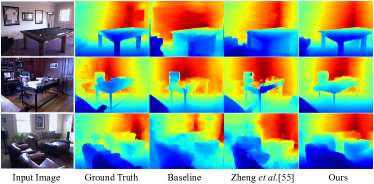
Figure 6: Qualitative comparison of the depth maps on the NYU Depth v2 dataset. Our method restores clear object boundaries, e.g., sofas and tables.

Table 5: Comparison of the contribution of each module with best results marked in bold.

	Higher is better			Lower is better
Method	$\delta<1.25$	$\delta<1.25^{2}$	$\delta<1.25^{3}$	Abs Rel	Squa Rel	RMSE	RMSElog
Baseline	0.642	0.861	0.944	0.236	2.171	7.063	0.315
+STE	0.730	0.903	0.958	0.201	1.989	6.606	0.273
+STE + DSA (Add)	0.751	0.915	0.968	0.185	1.715	6.214	0.257
+STE + DSA (Concat)	0.753	0.919	0.970	0.179	1.487	5.975	0.252
+STE + DSA ($\otimes$)	0.781	0.931	0.972	0.165	1.351	5.695	0.236
Edge + Baseline	0.688	0.887	0.957	0.217	1.970	6.674	0.285
Segmentation Map + Baseline	0.689	0.901	0.965	0.204	1.645	6.240	0.274

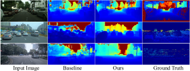
Figure 7: Qualitative results on the cross-datasets. From top to bottom: Cityscapes/DrivingStereo/nuScenes.

We also visualize the representations in Figure 5. Interestingly, our depth-specific representations focus on the layout, junctions and object boundaries of indoor scenes. It is worth noting that the boundaries here are not edge maps but some important boundaries that can clearly reflect the geometric structure of the object. Compared with the structure map, the depth-specific structure map suppresses a large number of structures that are not related to depth information, such as photos on the wall and the texture structure of the floor, etc. Similar characteristics are observed for NYU Depth v2. This also validates that the structural representations reflect the most essential information of depth estimation, which can be effectively transfered between various domains. In Figure 6, we provide qualitative comparisons showing that our results are visually better that other methods. For example, the tables in the first and third rows and the sofas in the second and fourth rows maintain the finer geometric structure and object boundaries.

Generalization Results on More Datasets

Here we further verify our method on the cross-dataset tasks, i.e., vKITTI $\rightarrow$ Cityscapes/DrivingStereo/nuScenes. These three target datasets are auto-driving scenes, but the domain gap is larger compared to vKITTI $\rightarrow$ KITTI due to the variety of camera, location, whether and so on. We follow the same setting as vKITTI $\rightarrow$ KITTI. As shown in Table 4 and Figure 7, even though the domain gap is larger, our method consistently achieves significantly better generalizabilty than the Baseline and UDA method T²Net. The improvements vary depending on the structural domain gap.

4.3 Ablation Study

For the outdoor datasets, we use the DP module with raw image input as our baseline. We present the results of vKITTI$\rightarrow$KITTI in Table 5. The performance is gradually improved by incorporating STE module and DSA module. More specifically, after adding STE module, all the metrics are improved by a large margin from the baseline, where $\delta<1.25$ is increased by $13.7\%$, Abs-Rel is reduced by $14.8\%$ and RMSE is reduced by $6.47\%$, which shows that removing the style information in the original images can effectively improve the generalization ability of the depth estimation task. After adding DSA module, the performance in all metrics has been further improved, $\textsl{i.e.},$ $\delta<1.25$ is increased by $6.99\%$, Abs-Rel is reduced by $17.9\%$ and RMSE is reduced by $13.8\%$, which shows that the removal of depth-irrelevant structures can further improve the generalization ability of the model.

We study two more combinations of structure map and attention map: addtion (+STE + DRA (Add) ) and concatenation (+STE + DRA (Concat)). As Table 5 shows, our element-wise multiplication model (+STE + DRA ($\otimes$)) is more effective, because we use the predicted attention map to weight the general structure, which can be regarded as a bottleneck, suppressing depth-irrelevant information and enhancing depth-specific information, while the addtion or concatenation operations introduce redundancy and can not act as the bottleneck effectively.

Intuitively, edge map and the semantic segmentation map can also be regarded as structural representations. For the edge map, we apply the Sobel operator [39] to acquire the edge maps corresponding to the vKITTI and KITTI images. For the semantic segmentation map, vKITTI dataset provides semantic labels, and we use one of the state-of-the-art semantic segmentation methods [59] to predict semantic segmentation maps for KITTI. As illustrated in Table 5, edge maps and semantic segmentation maps can indeed improve the generalization ability of the network. Since our depth-specific representations only contains the most essential information for depth estimation, they have greater advantages over edge maps and semantic segmentation maps

In addition, we provide ablation study of our method in indoor scenes on SUNCG [40] and NYU Depth v2 [38] datasets in Table 3. We observe similar trends as reported in the outdoor scenario. Specifically, by adding STE module, the performance of our method has been greatly improved. After adding DSA module, the performance has been further improved. It is worth noting that the encoder part of our STE module uses the parameters trained on vKITTI (outdoor scenes) and PBN dataset. Although the indoor and outdoor scenes are very different, STE module can still work well in indoor scenes and learn the corresponding structure map of the indoor scenes.

5 Conclusion

In this paper, we present a novel structural representation for generalizable depth estimation. Our learnt representation can be well generalized to unseen real-world images when trained on synthetic data, though there is an obvious style gap. The key is to extract structure information which is disentangled from various domain styles. Since the extracted structure map only contains low-level general structures including a large amount of depth-irrelevant ones, we further propose the DSA module to extract complementary high-level semantic information from image to suppress depth-irrelevant content. The depth-specific structure map works as an information bottleneck and forces the network to infer depth from these essential representations rather than raw images. We even achieve better performance on unseen real-world images than the state-of-the-art domain adaptation methods which uses the real images from target domain for training. As for the limitation, we still need the scenarios (e.g. indoor or outdoor) to be similar between the synthetic and real-world images. This can be addressed by using a general synthetic dataset with various scenarios.

Acknowledgement

This work was supported in part by the National Natural Science Foundation of China (NSFC) under Grant 61632006 and Grant 62076230; in part by the Fundamental Research Funds for the Central Universities under Grant WK3490000003; and in part by Microsoft Research Asia.

Appendix

Figure 1: An overview of training process the encoder of STE module.

Appendix A Implementation details of encoder $\mathcal{E}_{s}$

We adopt an image translation framework [20] to train the encoder $\mathcal{E}_{s}$ of the STE module, as shown in Figure 1. To make the $\mathcal{E}_{s}$ generalizable to various style images, we choose the Painter By Numbers (PBN) dataset with a large style variation as the target domain for image translation and a synthetic dataset as the source domain. Given a source domain image $x^{s}$ and a target domain image $x^{t}$, we first use a shared $\mathcal{E}_{s}$ to extract the structure code for both the source and target domains denoted as $c_{a}^{s}$ and $c_{a}^{t}$ respectively. Then the domain specific style encoders $\mathcal{E}_{style}^{s}$ and $\mathcal{E}_{style}^{t}$ generate style codes $c_{b}^{s}$ and $c_{b}^{t}$ for the source and target domains respectively. The encoded structure code and style code are complementary for each domain. Combining these two codes, the original images from source and target domains can be restored by decoders $G_{s}$ and $G_{t}$ respectively. In addition, we also combine $c_{a}^{s}$ extracted from the source domain dataset with a randomly sampled style latent code $c_{b}^{t}$ from the prior distribution $q(c_{b}^{t})\sim\mathcal{N}(0,I)$. We use $G_{t}$ to produce the final output image $x_{s\to t}$. Similarly, we also combine $c_{a}^{t}$ extracted from the target domain dataset with a randomly sampled style latent code $c_{b}^{s}$ from the prior distribution $q(c_{b}^{s})\sim\mathcal{N}(0,I)$. $G_{s}$ is used to produce the final output image $x_{t\to s}$.

Given an image sampled from the data distribution, because the two parts are complementary, we decode them back to the original image by minimizing

$$\autobreak\mathcal{L}_{recon}^{x^{s}}=\mathbb{E}_{x^{s}\sim p(x^{s})}[||\mathcal{G}_{s}(\mathcal{E}_{s}(x^{s}),\mathcal{E}_{style}^{s}(x^{s}))-x^{s}||_{1}].$$ (1)

After obtaining the final image $x_{s\to t}$ through cross-domain translation, we input it to the shared structure encoder and the specific style encoder, so that the obtained latent code can also be reconstructed by minimizing

$$\autobreak\mathcal{L}_{recon}^{c_{a}^{s}}=\mathbb{E}_{c_{a}^{s}\sim p(c_{a}^{s}),c_{b}^{t}\sim q(c_{b}^{t})}[||\mathcal{E}_{s}(\mathcal{G}_{t}(c_{a}^{s},c_{b}^{t}))-c_{a}^{s}||_{1}],$$ (2)

and

$$\autobreak\mathcal{L}_{recon}^{c_{b}^{t}}=\mathbb{E}_{c_{a}^{s}\sim p(c_{a}^{s}),c_{b}^{t}\sim q(c_{b}^{t})}[||\mathcal{E}_{style}^{t}(\mathcal{G}_{t}(c_{a}^{s},c_{b}^{t}))-c_{b}^{t}||_{1}],$$ (3)

where $q({c_{b}^{t}})$ is the prior $N(0,I)$. We also use the adversarial loss to match the distribution of the translated images to the PBN data distribution as

$$\autobreak\mathcal{L}_{adv}^{x^{t}}=\mathbb{E}_{c_{a}^{s}\sim p(c_{a}^{s}),c_{b}^{t}\sim q(c_{b}^{t})}[log(1-D_{t}(x_{s\to t}))]+\mathbb{E}_{x_{t}\sim p(x_{t})}[logD_{t}(x_{t})],$$ (4)

where $D_{t}$ is a discriminator that tries to distinguish translated images from painting images. For the other branch, we follow similar pipeline to design the losses. By minimizing these loss functions, the structure code and style code of the image can be effectively disentangled. The total training objective is:

$$\min\limits_{(\mathcal{E}_{s},\mathcal{G}_{s},\mathcal{G}_{t},D_{s},D_{t})} \max\limits_{(D_{s},D_{t})}\mathcal{L}_{total}=$$

$$\mathcal{L}_{adv}^{x^{s}}+\mathcal{L}_{adv}^{x^{t}}+\lambda_{1}(L_{recon}^{x^{s}}+L_{recon}^{x^{t}})+$$

$$\lambda_{2}(\mathcal{L}_{recon}^{c_{b}^{t}}+L_{recon}^{c_{a}^{s}})+$$ (5)

$$\lambda_{3}(\mathcal{L}_{recon}^{c_{b}^{s}}+L_{recon}^{c_{a}^{t}}),$$

where $\lambda_{1},\lambda_{2},\lambda_{3}$ are weights for the three losses respectively.

Appendix B Visualize structure maps of images with different styles but the same structure code

We show the structure maps of images with different styles but the same structure codes in Figure 2. The structure maps are generated by feeding images of different styles but same structure code into the STE module. It can be seen from Figure 2 that although the image styles are different, the generated structure maps are very similar, which further proves that the STE module can ignore the style information and only extract the structure information.

Appendix C Performance on NYU Depth v2 for semi-supervised setting

We show the performance of our method under the semi-supervised setting on NYU Depth v2 in Table 1. It can be seen from Table 1 that even though our method only uses 500 labeled real data (0.42$\%$ of the total dataset) to fine-tune the domain generalization model, our method outperforms semi-supervised methods [54] under the same settings, and even outperforms some fully supervised methods [28, 7]. It is worth noting that Laina et al.[27] use more than 120k data to train the depth predictor, and we still surpass their approach on the RMSE.

Appendix D Datasets and Evaluating Metrics

In the following section, we will introduce these datasets and evaluating metrics used in our experiments in detail.

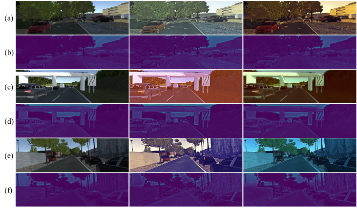
Figure 2: Visualize structure maps of different styles and the same structure code. (a), (c) and (e) represent the images of different styles under the same structure code. (b), (d) and (f) are the generated structure maps.

vKITTI [9]

is a photo-realistic synthetic dataset, that contains 21260 image-depth paired generated from five different virtual worlds in diverse urban settings and weather conditions. The image resolution of this dataset is $375\times 1242$. To train our network, we follow prior works [55, 53], to randomly select 20760 image-depth pairs as our train datasets. We downsample all the images to $192\times 640$ and data augmentation is conducted including random horizontal flipping with a probability of $0.5$, rotation with degrees in $[-5^{\circ},5^{\circ}]$, and brightness adjustment. Because the ground truth of KITTI and vKITTI are significantly different, the maximum depth of the vKITTI dataset is $655.35m$, and the maximum depth value of KITTI is $80m$. In order to reduce the influence of ground truth differences, the depth value of vKITTI is usually clipped to $80m$ [55, 25].

SUNCG [40]

is an indoor synthetic dataset, which contains 45622 3D houses with various room types. The image size is $480\times 640$. Following previous studies [55], we chose the camera locations, poses, and parameters based on the distribution of real NYU Depth v2 dataset [38] and retained valid depth maps using the same criteria as Zheng et al.[55]. 130190 image-depth pairs are downsampled to $192\times 256$ and used for training.

Table 1: Performance on NYU Depth v2 for semi-supervised setting with best results marked in bold.

Method	Abs Rel	RMSE	$\log{10}$	$\delta<1.25$	$\delta<1.25^{2}$	$\delta<1.25^{3}$
Li et al.[28]	0.232	0.821	0.094	0.621	0.886	0.968
Eigen et al.[7]	0.215	0.907	-	0.611	0.887	0.971
Laina et al.[27]	0.127	0.573	0.055	0.811	0.953	0.988
Zhao et al.[54]	0.186	0.710	-	0.712	0.917	0.977
Ours	0.168	0.544	0.069	0.764	0.945	0.984

KITTI [13]

is an outdoor real dataset, which is built for various computer vision tasks for autonomous driving. The images and depth maps are captured for outdoor scenes through a LiDAR sensor deployed on a driving vehicle. The original image resolution is $375\times 1241$.

NYU Depth v2 [38]

is a real indoor dataset, which contains 464 video sequences of indoor scenes captured with Microsoft Kinect. The dataset is wildly used to evaluate monocular depth estimation tasks for indoor scenes. Following previous work [55, 25, 17, 3], we use the official 654 aligned image-depth pairs for evaluation. The image resolution is $480\times 640$.

Evaluating Metrics

To quantitatively evaluate the proposed approach, we follow previous work [7, 8, 27, 58]. The evaluation metrics include root mean squared error (RMSE), mean relative error (REL), Mean $\log 10$ error ($\log 10$), root mean squared error in $\log$ space (RMSE_log), and squared relative error (Squa-Rel), defined as:

• RMSE: $\sqrt{\frac{1}{N}\sum_{i=1}^{N}(d_{i}-\hat{d}_{i})^{2}}$.

• REL: $\frac{1}{N}\sum_{i=1}^{N}\frac{|d_{i}-\hat{d}_{i}|}{\hat{d}_{i}}$.

• Mean $\log 10$ error ($\log 10$): $\frac{1}{N}\sum_{i=1}^{N}|\log_{10}d_{i}-\log_{10}\hat{d}_{i}|$.

• RMSE_log: $\sqrt{\frac{1}{N}\sum_{i=1}^{N}(\log d_{i}-\log\hat{d}_{i})^{2}}$.

• Squa-Rel: $\frac{1}{N}\sum_{i=1}^{N}\frac{|d_{i}-\hat{d}_{i}|^{2}}{\hat{d}_{i}}$.

• Accuracy with threshold $t$: Percentage of pixels whose depth $d_{i}$ satisfies $\max\big{(}\frac{d_{i}}{\hat{d}_{i}},\frac{\hat{d}_{i}}{d_{i}}\big{)}=\delta<t$, where $t\in[1.25,1.25^{2},1.25^{3}]$ respectively.

$d_{i}$ and $\hat{d}_{i}$ are the predicted depth and ground-truth depth at pixel $i$ respectively. $N$ denotes the number of valid pixels in the ground-truth depth map.

References

- [1] Amir Atapour-Abarghouei and Toby P Breckon. Real-time monocular depth estimation using synthetic data with domain adaptation via image style transfer. In CVPR, 2018.
- [2] Holger Caesar, Varun Bankiti, Alex H Lang, Sourabh Vora, Venice Erin Liong, Qiang Xu, Anush Krishnan, Yu Pan, Giancarlo Baldan, and Oscar Beijbom. nuscenes: A multimodal dataset for autonomous driving. In CVPR, 2020.
- [3] Xiaotian Chen, Xuejin Chen, and Zheng-Jun Zha. Structure-aware residual pyramid network for monocular depth estimation. In IJCAI, 2019.
- [4] Yuhua Chen, Cordelia Schmid, and Cristian Sminchisescu. Self-supervised learning with geometric constraints in monocular video: Connecting flow, depth, and camera. In ICCV, 2019.
- [5] Marius Cordts, Mohamed Omran, Sebastian Ramos, Timo Rehfeld, Markus Enzweiler, Rodrigo Benenson, Uwe Franke, Stefan Roth, and Bernt Schiele. The cityscapes dataset for semantic urban scene understanding. In CVPR, 2016.
- [6] David Eigen and Rob Fergus. Predicting depth, surface normals and semantic labels with a common multi-scale convolutional architecture. In ICCV, 2015.
- [7] David Eigen, Christian Puhrsch, and Rob Fergus. Depth map prediction from a single image using a multi-scale deep network. In NeurIPS, 2014.
- [8] Huan Fu, Mingming Gong, Chaohui Wang, Kayhan Batmanghelich, and Dacheng Tao. Deep ordinal regression network for monocular depth estimation. In CVPR, 2018.
- [9] Adrien Gaidon, Qiao Wang, Yohann Cabon, and Eleonora Vig. Virtual worlds as proxy for multi-object tracking analysis. In CVPR, 2016.
- [10] Yaroslav Ganin and Victor Lempitsky. Unsupervised domain adaptation by backpropagation. In ICML, 2015.
- [11] Ravi Garg, BG Vijay Kumar, Gustavo Carneiro, and Ian Reid. Unsupervised cnn for single view depth estimation: Geometry to the rescue. In ECCV, 2016.
- [12] Leon A Gatys, Alexander S Ecker, and Matthias Bethge. Image style transfer using convolutional neural networks. In CVPR, 2016.
- [13] Andreas Geiger, Philip Lenz, Stiller Christoph, and Raquel Urtasun. Vision meets robotics: The kitti dataset. IJRR, 2013.
- [14] Clément Godard, Oisin Mac Aodha, and Gabriel J. Brostow. Unsupervised monocular depth estimation with left-right consistency. In CVPR, 2017.
- [15] Clément Godard, Oisin Mac Aodha, Michael Firman, and Gabriel J. Brostow. Digging into self-supervised monocular depth prediction. In ICCV, 2019.
- [16] Vitor Guizilini, Rui Hou, Jie Li, Rares Ambrus, and Adrien Gaidon. Semantically-guided representation learning for self-supervised monocular depth. In ICLR, 2019.
- [17] Junjie Hu, Mete Ozay, Yan Zhang, and Takayuki Okatani. Revisiting single image depth estimation: Toward higher resolution maps with accurate object boundaries. In WACV, 2019.
- [18] Junjie Hu, Yan Zhang, and Takayuki Okatani. Visualization of convolutional neural networks for monocular depth estimation. In ICCV, 2019.
- [19] Xun Huang and Serge Belongie. Arbitrary style transfer in real-time with adaptive instance normalization. In ICCV, 2017.
- [20] Xun Huang, Ming-Yu Liu, Serge Belongie, and Jan Kautz. Multimodal unsupervised image-to-image translation. In ECCV, 2018.
- [21] Sunghoon Im, Hae-Gon Jeon, Steve Lin, and Kweon In-So. Dpsnet: End-to-end deep plane sweep stereo. In ICLR, 2019.
- [22] Phillip Isola, Jun-Yan Zhu, Tinghui Zhou, and Alexei A Efros. Image-to-image translation with conditional adversarial networks. In CVPR, 2017.
- [23] Xin Jin, Cuiling Lan, Wenjun Zeng, Zhibo Chen, and Li Zhang. Style normalization and restitution for generalizable person re-identification. In CVPR, 2020.
- [24] Hadi Kazemi, Seyed Mehdi Iranmanesh, and Nasser M. Nasrabadi. Style and content disentanglement in generative adversarial networks. In WACV, 2019.
- [25] Jogendra Nath Kundu, Phani Krishna Uppala, Anuj Pahuja, and R. Venkatesh Babu. Adadepth: Unsupervised content congruent adaptation for depth estimation. In CVPR, 2018.
- [26] Yevhen Kuznietsov, Jorg Stuckler, and Bastian Leibe. Semi-supervised deep learning for monocular depth map prediction. In CVPR, 2017.
- [27] Iro Laina, Christian Rupprecht, Vasileios Belagiannis, Federico Tombari, and Nassir Navab. Deeper depth prediction with fully convolutional residual networks. In 3DV, 2016.
- [28] Bo Li, Chunhua Shen, Yuchao Dai, Anton Van Den Hengel, and Mingyi He. Depth and surface normal estimation from monocular images using regression on deep features and hierarchical CRFs. In CVPR, 2015.
- [29] Fayao Liu, Chunhua Shen, Guosheng Lin, and Ian Reid. Learning depth from single monocular images using deep convolutional neural fields. IEEE TPAMI, 2015.
- [30] Mingsheng Long, Han Zhu, Jianmin Wang, and Michael I Jordan. Unsupervised domain adaptation with residual transfer networks. In NeurIPS, 2016.
- [31] Krikamol Muandet, David Balduzzi, and Bernhard Schölkopf. Domain generalization via invariant feature representation. In ICML, 2013.
- [32] Xingang Pan, Ping Luo, Jianping Shi, and Xiaoou Tang. Two at once: Enhancing learning and generalization capacities via ibn-net. In ECCV, 2018.
- [33] Adam Paszke, Sam Gross, Soumith Chintala, Gregory Chanan, Edward Yang, Zachary DeVito, Zeming Lin, Alban Desmaison, Luca Antiga, and Adam Lerer. Automatic differentiation in pytorch. In NeurIPSW, 2017.
- [34] Xiaojuan Qi, Renjie Liao, Zhengzhe Liu, Raquel Urtasun, and Jiaya Jia. Geonet: Geometric neural network for joint depth and surface normal estimation. In CVPR, 2018.
- [35] Xiaojuan Qi, Zhengzhe Liu, Renjie Liao, Philip HS Torr, Raquel Urtasun, and Jiaya Jia. Geonet++: Iterative geometric neural network with edge-aware refinement for joint depth and surface normal estimation. IEEE TPAMI, 2020.
- [36] Kuniaki Saito, Kohei Watanabe, Yoshitaka Ushiku, and Tatsuya Harada. Maximum classifier discrepancy for unsupervised domain adaptation. In CVPR, 2018.
- [37] Shiv Shankar, Vihari Piratla, Soumen Chakrabarti, Siddhartha Chaudhuri, Preethi Jyothi, and Sunita Sarawagi. Generalizing across domains via cross-gradient training. In ICLR, 2018.
- [38] Nathan Silberman, Derek Hoiem, Pushmeet Kohli, and Rob Fergus. Indoor segmentation and support inference from RGBD images. In ECCV, 2012.
- [39] Irwin Sobel and Gary Feldman. A 3x3 isotropic gradient operator for image processing. SAIL, 1973.
- [40] Shuran Song, Fisher Yu, Andy Zeng, Angel X Chang, Manolis Savva, and Thomas Funkhouser. Semantic scene completion from a single depth image. In CVPR, 2017.
- [41] Maxim Tatarchenko, Stephan R. Richter, René Ranftl, Zhuwen Li, Vladlen Koltun, and Thomas Brox. What do single-view 3d reconstruction networks learn? In CVPR, 2019.
- [42] Lijun Wang, Jianming Zhang, Oliver Wang, Zhe Lin, and Huchuan Lu. Sdc-depth: Semantic divide-and-conquer network for monocular depth estimation. In CVPR, 2020.
- [43] Jamie Watson, Michael Firman, Gabriel J Brostow, and Daniyar Turmukhambetov. Self-supervised monocular depth hints. In ICCV, 2019.
- [44] Fei Xia, Amir R. Zamir, Zhi-Yang He, Alexander Sax, Jitendra Malik, and Silvio Savarese. Gibson Env: real-world perception for embodied agents. In CVPR, 2018.
- [45] Zhihao Xia, Patrick Sullivan, and Ayan Chakrabarti. Generating and exploiting probabilistic monocular depth estimates. In CVPR, 2020.
- [46] Dan Xu, Elisa Ricci, Wanli Ouyang, Xiaogang Wang, and Nicu Sebe. Multi-scale continuous CRFs as sequential deep networks for monocular depth estimation. In CVPR, 2017.
- [47] Dan Xu, Wei Wang, Hao Tang, Hong Liu, Nicu Sebe, and Elisa Ricci. Structured attention guided convolutional neural fields for monocular depth estimation. In CVPR, 2018.
- [48] Guorun Yang, Xiao Song, Chaoqin Huang, Zhidong Deng, Jianping Shi, and Bolei Zhou. Drivingstereo: A large-scale dataset for stereo matching in autonomous driving scenarios. In CVPR, 2019.
- [49] Yao Yao, Zixin Luo, Shiwei Li, Tian Fang, and Long Quan. Mvsnet: Depth inference for unstructured multi-view stereo. In ECCV, 2018.
- [50] Wei Yin, Yifan Liu, Chunhua Shen, and Youliang Yan. Enforcing geometric constraints of virtual normal for depth prediction. In ICCV, 2019.
- [51] Zhichao Yin and Jianping Shi. Geonet: Unsupervised learning of dense depth, optical flow and camera pose. In CVPR, 2018.
- [52] Fisher Yu, Vladlen Koltun, and Thomas Funkhouser. Dilated residual networks. In CVPR, 2017.
- [53] Shanshan Zhao, Huan Fu, Mingming Gong, and Dacheng Tao. Geometry-aware symmetric domain adaptatizhaoon for monocular depth estimation. In CVPR, 2019.
- [54] Yunhan Zhao, Shu Kong, Daeyun Shin, and Charless Fowlkes. Domain decluttering: Simplifying images to mitigate synthetic-real domain shift and improve depth estimation. In CVPR, 2020.
- [55] Chuanxia Zheng, Tat-Jen Cham, and Jianfei Cai. T2net: Synthetic-to-realistic translation for solving single-image depth estimation tasks. In ECCV, 2018.
- [56] Junsheng Zhou, Yuwang Wang, Qin Kaihuai, and Wenjun Zeng. Unsupervised high-resolution depth learning from videos with dual networks. In ICCV, 2019.
- [57] Junsheng Zhou, Yuwang Wang, Kaihuai Qin, and Wenjun Zeng. Moving indoor: Unsupervised video depth learning in challenging environments. In ICCV, 2019.
- [58] Tinghui Zhou, Brown Matthew, Snavely Noah, and David G. Lowe. Unsupervised learning of depth and ego-motion from video. In CVPR, 2017.
- [59] Yi Zhu, Karan Sapra, Fitsum A. Reda, Kevin J. Shih, Shawn Newsam, Andrew Tao, and Bryan Catanzaro. Improving semantic segmentation via video propagation and label relaxation. In CVPR, 2019.
- [60] Wei Zhuo, Mathieu Salzmann, Xuming He, and Miaomiao Liu. Indoor scene structure analysis for single image depth estimation. In CVPR, 2015.