Supplementary Information:
Constrained non-negative matrix factorization enabling real-time insights of in situ and high-throughput experiments

I Partially constraining components with synthetic datasets

When considering the dataset shown in the main text Figure 1b, knowing even some of the underlying components increases the effectiveness of the NMF decomposition.

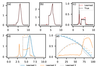
Figure 1: The reconstruction of the (a) first, (b) median, and (c) last pattern of a dataset of mixed Gaussian, Lorenzian, and box functions using constrained NMF. (d) Prior knowledge of the Gaussian function fixes one underlying component. (e) The learned weights are improved and create an better reconstruction of the dataset, than canonical NMF (MSE=13.314, R-factor=0.029).

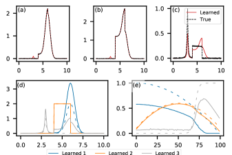
Figure 2: The reconstruction of the (a) first, (b) median, and (c) last pattern of a dataset of mixed Gaussian, Lorenzian, and box functions using constrained NMF. (d) Prior knowledge of the box function fixes one underlying component. (e) The learned weights are improved and create an better reconstruction of the dataset, than canonical NMF (MSE=27.959, R-factor=0.044).

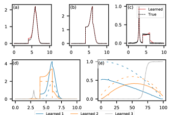
Figure 3: The reconstruction of the (a) first, (b) median, and (c) last pattern of a dataset of mixed Gaussian, Lorenzian, and box functions using constrained NMF. (d) Prior knowledge of the Lorenzian function fixes one underlying component. (e) The learned weights are improved and create an better reconstruction of the dataset, than canonical NMF (MSE=3.838, R-factor=0.018).

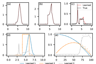
Figure 4: The reconstruction of the (a) first, (b) median, and (c) last pattern of a dataset of mixed Gaussian, Lorenzian, and box functions using constrained NMF. (d) Prior knowledge of the Gaussian and box functions fixes two underlying components. (e) The learned weights are improved and create an better reconstruction of the dataset, than canonical NMF (MSE=3.788, R-factor=0.020).

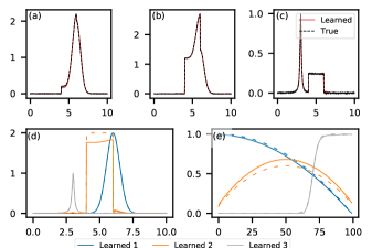
Figure 5: The reconstruction of the (a) first, (b) median, and (c) last pattern of a dataset of mixed Gaussian, Lorenzian, and box functions using constrained NMF. (d) Prior knowledge of the Gaussian and Lorenzian functions fixes two underlying components. (e) The learned weights are improved and create an better reconstruction of the dataset, than canonical NMF (MSE=1.752, R-factor=0.015).

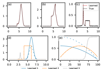
Figure 6: The reconstruction of the (a) first, (b) median, and (c) last pattern of a dataset of mixed Gaussian, Lorenzian, and box functions using constrained NMF. (d) Prior knowledge of the box and Lorenzian functions fixes two underlying components. (e) The learned weights are improved and create an better reconstruction of the dataset, than canonical NMF (MSE=2.159, R-factor=0.015).

II Constraints enable physically meaningful in situ analysis of melting salts using the pair distribution function

The results from the pair distribution function (PDF) analysis mirror that of the X-ray diffraction (XRD) results in the main text. The primary difference is the noise persistent in the resultant components, which is necessary to recreate the dataset. Since PDF is a calculated function from the integrated total scattering, it requires an additional step in the data stream to reduce the reciprocal space function into a real space PDF. This imperfect data reduction on-the-fly created a lack of uniformity at large radii for the amorphous regions. In this case, the function G(r) was used, pre-processed for NMF by min-max normalization.

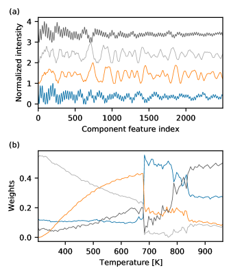
Figure 7: Canonical NMF produces a confusing decomposition, offering limited clarity to the scientist. (a) The learned components are non-physical and cannot be interpreted as PDFs. (b) The learned weights provide little information beyond an abrupt change around 400  K.

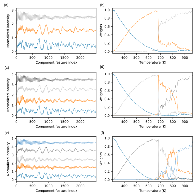
Figure 8: Automated constrained NMF was run using 3-6 components asynchronously on the molten salt dataset for PDFs. The learned components for the (a) 3, (c) 4, and (e) 6 component decompostions provide insight into thermal expansion, a phases present during the temperature ramp. The learned weights for the (b) 3, (d) 4, and (f) 6 component decompositions demonstrate the second-order phase transition, the characteristic response to thermal expansion, and persistence of a solid phase after 400  K.