Poisson Phase Retrieval
in Very Low-count Regimes

Abstract

This paper discusses phase retrieval algorithms for maximum likelihood (ML) estimation from measurements following independent Poisson distributions in very low-count regimes, e.g., 0.25 photon per pixel. To maximize the log-likelihood of the Poisson ML model, we propose a modified Wirtinger flow (WF) algorithm using a step size based on the observed Fisher information. This approach eliminates all parameter tuning except the number of iterations. We also propose a novel curvature for majorize-minimize (MM) algorithms with a quadratic majorizer. We show theoretically that our proposed curvature is sharper than the curvature derived from the supremum of the second derivative of the Poisson ML cost function. We compare the proposed algorithms (WF, MM) with existing optimization methods, including WF using other step-size schemes, quasi-Newton methods such as LBFGS and alternating direction method of multipliers (ADMM) algorithms, under a variety of experimental settings. Simulation experiments with a random Gaussian matrix, a canonical DFT matrix, a masked DFT matrix and an empirical transmission matrix demonstrate the following. 1) As expected, algorithms based on the Poisson ML model consistently produce higher quality reconstructions than algorithms derived from Gaussian noise ML models when applied to low-count data. Furthermore, incorporating regularizers, such as corner-rounded anisotropic total variation (TV) that exploit the assumed properties of the latent image, can further improve the reconstruction quality. 2) For unregularized cases, our proposed WF algorithm with Fisher information for step size converges faster (in terms of cost function and PSNR vs. time) than other WF methods, e.g., WF with empirical step size, backtracking line search, and optimal step size for the Gaussian noise model; it also converges faster than the LBFGS quasi-Newton method. 3) In regularized cases, our proposed WF algorithm converges faster than WF with backtracking line search, LBFGS, MM and ADMM.

I Introduction

Phase retrieval is an inverse problem with many applications in engineering and applied physics [1, 2], including radar [3], X-ray crystallography [4], astronomical imaging [5], Fourier ptychography [6, 7, 8, 9] and coherent diffractive imaging (CDI) [10]. In these applications, the sensing systems can only measure the magnitude (or the square of the magnitude) of the signal, for example, optical detection devices (e.g., CCD cameras) cannot measure the phase of a light wave. The problem of recovering the original signal from only the magnitude of such linear measurements is called phase retrieval. Mathematically, the goal is to recover the unknown signal $\bm{x}\in\mathbb{F}^{N}$ from measurements $\{y_{i}\}$ that follow some statistical distribution

$$y_{i}\sim p(|\bm{a}_{i}^{\prime}\bm{x}|^{2}+b_{i}),$$ (1)

where $p(\cdot)$ is a probability density function. Here, $\bm{a}_{i}^{\prime}\in\mathbb{C}^{N}$ denotes the $i$th row of the system matrix $\bm{A}\in\mathbb{C}^{M\times N}$, where $i=1,\ldots,M$, and $b_{i}\in\mathbb{R}_{+}$ denotes a known mean background signal for the $i$th measurement, e.g., as arising from dark current [11]. Here the field $\mathbb{F}=\mathbb{R}$ or $\mathbb{F}=\mathbb{C}$ depending on whether $\bm{x}$ is known to be real or complex.

The sensing vectors $\{\bm{a}_{i}^{\prime}\}$ are often assumed to follow some structure, e.g., i.i.d. random Gaussian, or the coefficients of discrete Fourier transform (DFT). For the random Gaussian case, Candès et al. [12] showed that $M\sim\mathcal{O}(N\log N)$ samples are sufficient to recover the signal; Bandeira et al. [13] posed a conjecture that $M=4N-4$ is necessary and sufficient to uniquely recover the original signal from noiseless measurements. However, under very low-count regimes with noise, a much larger $M$ is often needed to successfully reconstruct the signal. Additionally, when $\bm{A}$ corresponds to a Fourier transform, the measurements describe only the magnitudes of a signal’s Fourier coefficients, and one usually does not have enough information to recover the signal; while the Fourier transform is injective, its point-wise absolute value is not [14]. So a common approach is to create redundancy in the measurement process by additional illuminations of the object using different masks [15]. Banderia et al. [14] showed that by using a set of $\mathcal{O}(\log M)$ random masks can increase the probability of recovering the signal.

I-A Background for Gaussian phase retrieval

In many previous works, the measurement vector $\bm{y}\in\mathbb{R}^{M}$ was assumed to have statistically independent elements following Gaussian distributions with variance $\sigma^{2}$:

$$y_{i}\sim\mathcal{N}(|\bm{a}_{i}^{\prime}\bm{x}|^{2}+b_{i},\sigma^{2}).$$ (2)

For this Gaussian noise model, the ML estimate of $\bm{x}$ corresponds to the following non-convex optimization problem

$$\hat{\bm{x}}=\operatorname*{arg\,min}_{\bm{x}\in\mathbb{F}^{N}}g(\bm{x}),\ g(\bm{x})\triangleq\sum_{i}\;\Big{|}y_{i}-b_{i}-\big{|}\bm{a}_{i}^{\prime}\bm{x}\big{|}^{2}\Big{|}^{2}.$$ (3)

To solve (3), numerous algorithms have been proposed. One approach reformulates (3) by “matrix lifting” [12, 15, 16], where a rank-one matrix is introduced and if the rank constraint is relaxed, then the transformed problem is convex and can be solved by semi-definite programming (SDP). The SDP based algorithms can yield robust solutions but can be computational expensive, especially on large-scale data. Another approach is Wirtinger Flow (WF) [17] and its variants [18, 19, 20] that descend the cost function with a (projected/thresholded/truncated) Wirtinger gradient using an appropriate step size. In the classic WF algorithm [17], the gradient for the Gaussian cost function (3) is

$$\nabla g(\bm{x})=4\bm{A}^{\prime}\operatorname{diag}\{|\bm{A}\bm{x}|^{2}-\bm{y}+{\bm{b}}\}\bm{A}\bm{x}.$$ (4)

To descend the cost function, reference [17] used a heuristic where the step size $\mu$ is rather small for the first few iterations and gradually increases as the iterations proceed. The intuition is that the gradient is noisy at the early iterations so a small step size is preferred. A drawback of this approach is that one needs to select hyper-parameters that control the growth of $\mu$. An alternative approach is to perform backtracking for $\mu$ at each iteration [21], i.e., by reducing $\mu$ until the cost function decreases sufficiently. This approach guarantees decreasing the cost function monotonically but can increase the compute time of the algorithm due to the variable number of inner iterations. Jiang et al. [18] derived the optimal step size for the Gaussian ML cost function (3) and showed faster convergence than the heuristic step size when measurements are noiseless or follow i.i.d. Gaussian distribution. Cai et al. [19] proposed thresholded WF and showed it can achieve the minimax optimal rates of convergence, but that scheme requires an appropriate selection of tuning parameters. Soltanolkotabi et al. [20] reformulated the phase retrieval problem as a nonconvex optimization problem and proved that projected Wirtinger gradient descent, when initialized in a neighborhood of the desired signal, has a linear convergence rate. However, it can be difficult to find an initial estimate satisfying the conditions mentioned in [20].

An alternative to cost function (3) (aka intensity model) is the magnitude model that works with the square root of $\bm{y}$. In particular, [22] proposed an algorithm known as Gerchberg Saxton (GS) that introduced a new variable $\bm{\theta}$ to represent the phase, leading to the following joint optimization problem

$$\hat{\bm{x}},\hat{\bm{\theta}}=\operatorname*{arg\,min}_{\bm{x}\in\mathbb{F}^{N},\,\bm{\theta}\in\mathbb{C}^{N}}\|\bm{A}\bm{x}-\operatorname{diag}\{\sqrt{\max(\bm{y}-{\bm{b}},\bm{0})}\}\,\bm{\theta}\|_{2}^{2},$$

$$\text{subject to}\quad|\theta_{i}|=1,\ i=1,...,N.$$ (5)

The square root in (I-A) is reminiscent of the Anscombe transform that converts a Poisson random variable into another random variable that approximately has a standard Gaussian distribution. However, that approximation is accurate when the Poisson mean is sufficiently large (e.g., above 5), whereas this paper focuses on the lower-count regime. The convergence and recovery guarantees of GS were studied in [23, 24].

In addition to matrix-lifting, WF, GS and their variants, several other algorithms have been proposed to solve phase retrieval problems under the assumption of the Gaussian measurement noise, including Gauss-Newton methods [25], LBFGS updates to approximate the Hessian in the Newton’s method [26], majorize-minimize (MM) methods [21], alternating direction method of multipliers (ADMM) [27], and an iterative soft-thresholding with exact line search algorithm (STELA) [28]. It seems unlikely that any of the many existing methods for the Gaussian noise case are optimal for low-count Poisson noise.

I-B Background for Poisson Phase Retrieval

In many low-photon count applications [29, 30, 8, 31, 32, 33, 34], especially in [34], where 0.25 photon per pixel on average is considered, a Poisson noise model is more appropriate:

$$y_{i}\sim\mathrm{Poisson}(|\bm{a}_{i}^{\prime}\bm{x}|^{2}+b_{i}).$$ (6)

ML estimation of $\bm{x}$ for the model (6) corresponds to the following optimization problem

$$\hat{\bm{x}}= \operatorname*{arg\,min}_{\bm{x}\in\mathbb{F}^{N}}f(\bm{x}),\quad f(\bm{x})\triangleq\sum_{i}\;\psi(\bm{a}_{i}^{\prime}\bm{x};y_{i},b_{i}),\quad$$

$$\psi(v;y,b)\triangleq(|v|^{2}+b)-y\log(|v|^{2}+b).$$ (7)

Here, $f(\bm{x})$ denotes the negative log-likelihood corresponding to (6), ignoring irrelevant constants independent of $\bm{x}$, and the function $\psi(\cdot;y,b)$ denotes the marginal negative log-likelihood for a single measurement, where $v\in\mathbb{C}$. Because $\left|v\right|$ is real, it is helpful to re-write $\psi$ in the form $\psi(v;y,b)=\phi(\left|v\right|;y,b),$ where

$$\phi(r;y,b)\triangleq(r^{2}+b)-y\log(r^{2}+b),\quad r\in\mathbb{R}_{+}.$$ (8)

One can verify that the function $\phi(r;y,b)$ is non-convex over $r\in\mathbb{R}_{+}$ when $0<b<y$. That property, combined with the modulus within the logarithm in (7), makes (7) a challenging optimization problem. Similar problems for $b=0$ have been considered previously [35, 6, 15, 36, 37], but many optical sensors also have Gaussian readout noise [7, 38] so that the mean background signal is unlikely to be zero. To accommodate the Gaussian readout noise, a more precise model would consider a sum of Gaussian and Poisson noise. However, the log likelihood for a Poisson plus Gaussian distribution is complicated, so a common approximation is to use a shifted Poisson model [39] that also leads to the cost function in (7). An alternative to the shifted Poisson model could be to work with an unbiased inverse transformation of a generalized Anscombe transform approximation [40, 9] or use a surrogate function that tightly upper bounds the challenging Poisson plus Gaussian ML objective function and apply a majorize-minimize algorithm [41]. Algorithms for the Poisson plus Gaussian noise model are interesting topics for future work.

Existing algorithms for the Poisson phase retrieval are limited in the literature. Chen et al. [36] proposed to solve the Poisson phase retrieval problem by minimizing a nonconvex functional as in the Wirtinger flow (WF) approach; Bian et al. [6] used Poisson ML estimation and truncated Wirtinger flow in Fourier ptychographic (FP) reconstruction. Zhang et al. [42] consider a scale square root of (6) for the common case with $b_{i}=0$. Chang et al. [43] derived a (TV) regularized ADMM algorithm for Poisson phase retrieval and established its convergence. Recently, Fatima et al. [44] proposed a double looped primal-dual majorize-minimize (PDMM) algorithm.

In this paper, we propose novel algorithms for the Poisson phase retrieval problem and report empirical comparisons of the convergence speed and reconstruction quality of algorithms under a variety of experimental settings. We presented a preliminary version of this work at the 2021 IEEE international conference on image processing (ICIP) [45]. We significantly extended this work by testing our proposed method under more practical experimental settings. We also added comparisons to related works such as [18, 26].

The main contributions of this paper can be summarized as follows:

1. We propose a novel method for computing the step size for the WF algorithm that can lead to faster convergence compared to empirical step size [17], backtracking line search [21], optimal step size derived for the Gaussian noise model [18], and LBFGS updates to approximate the Hessian in Newton’s method [26]. Moreover, our proposed method can be computed efficiently without any tuning parameter.

2. We derive a majorize-minimize (MM) algorithm with quadratic majorizer using a novel curvature. We show theoretically that our proposed curvature is sharper than the curvature derived from the upper bound of the second derivative of the Poisson ML cost function.

3. We present numerical simulation results under random Gaussian, canonical DFT, masked DFT and empirical transmission system matrix settings for very low-count data, e.g., 0.25 photon per pixel. We show that under such experimental settings, algorithms derived from the Poisson ML model produce consistently higher reconstruction quality than algorithms derived from Gaussian ML model, as expected. Furthermore, the reconstruction quality is further improved by incorporating regularizers that exploit assumed properties of the signal.

4. We compare the convergence speed (in terms of cost function and PSNR vs. time) of WF with Fisher information with other methods for step size (backtracking line search, optimal Gaussian) and LBFGS quasi-Newton method. We also compare the convergence speed of regularized WF with MM and ADMM [46], using smooth regularizers such as corner-rounded anisotropic total variation (TV). For both cases, our proposed WF Fisher algorithm converges the fastest under all system matrix settings.

The rest of this paper is organized as follows. Section II introduces the proposed modified WF method with Fisher information for step size; and derives the improved curvature for the MM algorithm. Section III illustrates implementation details of algorithms discussed in Section II. Section IV provides numerical results using simulated data under different experimental settings. Section V and section VI discuss and conclude this paper and provide future directions.

Notation: Bold upper/lower case letters (e.g., $\bm{A}$, $\bm{x}$, $\bm{y}$, $\bm{b}$) denote matrices and column vectors, respectively. Italics (e.g., $\mu,y,b$) denote scalars. $y_{i}$ and $b_{i}$ denote the $i$th element in vector $\bm{y}$ and $\bm{b}$, respectively. $\mathbb{R}^{N}$ and $\mathbb{C}^{N}$ denote $N$-dimensional real/complex normed vector space, respectively. $(\cdot)^{*}$ denotes the complex conjugate and $(\cdot)^{\prime}$ denotes Hermitian transpose. $\operatorname{diag}\{\cdot\}$ is a diagonal matrix constructed from a column vector. Unless otherwise defined, a subscript denotes outer iterations and superscript denotes the inner iterations, respectively. For example, $\bm{x}_{k}$ denotes the estimate of $\bm{x}$ at the $k$th iteration of an algorithm. $\varoslash$ denotes element-wise division. The first and second derivatives of a scalar function $\psi$ are denoted $\dot{\psi}$ and $\ddot{\psi}$, respectively. For gradients associated with complex numbers/vectors, the notation $\dot{\psi}(\cdot)$ and $\nabla(\cdot)$, should be considered as an ascent direction, not as a derivative.

II Methods

II-A Wirtinger flow (WF)

This section describes the modified WF algorithm with proposed step-size approach based on Fisher information. To generalize the Wirtinger flow algorithm to the Poisson cost function (7), the most direct approach simply replaces the gradient (4) by (II-A) in the WF framework [42] and performs backtracking to find the step-size $\mu$, as in [21]. We propose a faster alternative next. We treat $0\log 0$ as $0$ in (7) because a Poisson random variable with zero mean can only take the value $0$. With this assumption, one can verify that $\psi$ has the following well-defined ascent direction (negative of descent direction [47]) and a second derivative:

$$\dot{\psi}(v;y,b)=2v\left(1-\frac{y}{|v|^{2}+b}\right),\quad v\in\mathbb{C}.$$

$$\ddot{\psi}(v;y,b)=\mathrm{sign}(v)\Bigg{(}2+2y\frac{|v|^{2}-b}{(|v|^{2}+b)^{2}}\Bigg{)},$$

$$|\ddot{\psi}(v;y,b)|\leq 2+\frac{y}{4b}.$$ (9)

II-A1 Fisher information for Poisson model

We first make a quadratic approximation along the gradient direction of the cost function at each iteration, and then apply one step of Newton’s method to minimize that 1D quadratic. Because computing the Hessian can be computationally expensive in large-scale problems, we follow the statistics literature by replacing the Hessian by the observed Fisher information when applying Newton’s method [48, 49]. Our Fisher approach is based on the fact that the observed Fisher information is the negative Hessian matrix of the incomplete data log-likelihood functions evaluated at the observed data, and hence can provide a good approximation to the Hessian with enough data [50]. Moreover, the Fisher information matrix is always positive semi-definite, and avoids calculation of second derivatives. Using Fisher information in gradient-based algorithms has a long history in statistics and is central to Fisher’s method of scoring [48, 51, 52, 49].

Specifically, we first approximate the 1D line search problem associated with (7) by the following Taylor series

$$\mu_{k} =\operatorname*{arg\,min}_{\mu\in\mathbb{R}}f_{k}(\mu),$$

$$f_{k}(\mu) \triangleq f(\bm{x}_{k}-\mu\nabla f(\bm{x}_{k}))\approx f(\bm{x}_{k})-\|\nabla f(\bm{x}_{k})\|_{2}^{2}\,\mu$$

$$\ +\frac{1}{2}\nabla f(\bm{x}_{k})^{\prime}\nabla^{2}f(\bm{x}_{k})\nabla f(\bm{x}_{k})\mu^{2},$$ (10)

where one can verify that the minimizer is

$$\mu_{k}=\frac{\|\nabla f(\bm{x}_{k})\|_{2}^{2}}{\nabla f(\bm{x}_{k})^{\prime}\nabla^{2}f(\bm{x}_{k})\nabla f(\bm{x}_{k})}.$$ (11)

We next approximate the Hessian matrix $\nabla^{2}f(\bm{x})$ using the observed Fisher information matrix:

$$\nabla^{2}f(\bm{x}) \approx\bm{I}(\bm{x},{\bm{b}})$$ (12)

$$\triangleq\mathbb{E}_{\bm{y}}\Big{[}\nabla^{2}f(\bm{x};\bm{y},{\bm{b}})\Big{|}\bm{x},{\bm{b}}\Big{]}$$

$$=\mathbb{E}_{\bm{y}}\Big{[}\big{(}\nabla f(\bm{x};\bm{y},{\bm{b}})\big{)}\big{(}\nabla f(\bm{x};\bm{y},{\bm{b}})\big{)}^{\prime}\Big{|}\bm{x},{\bm{b}}\Big{]}$$

$$=\bm{A}^{\prime}\mathbb{E}_{\bm{y}}\Big{[}\big{(}\dot{\psi}_{\bm{\cdot}}(\bm{v};\bm{y},{\bm{b}})\big{)}\big{(}\dot{\psi}_{\bm{\cdot}}(\bm{v};\bm{y},{\bm{b}})\big{)}^{\prime}\Big{|}\bm{v},{\bm{b}}\Big{]}\bm{A}.$$

Here the dot subscript notation $\dot{\psi}_{\bm{\cdot}}(\bm{v};\bm{y},{\bm{b}})$ denotes element-wise application of the function $\dot{\psi}$ to its arguments (as in the Julia language), so the gradient $\dot{\psi}_{\bm{\cdot}}(\bm{v};\bm{y},{\bm{b}})$ is a vector in $\mathbb{C}^{M}$. One can verify that the marginal Fisher information for a single term $\psi(v;y,b)$ is

$$\bar{I}(v,b) =\mathbb{E}_{y}\Big{[}\big{|}\dot{\psi}(v;y,b)\big{|}^{2}\Big{|}v,b\Big{]}$$

$$=\frac{4|v|^{2}}{|v|^{2}+b},\quad v\in\mathbb{C},\ b>0.$$ (13)

Substituting (II-A1) into (12) using the statistical independence of the elements of the gradient vector, and then substituting (12) into (11) yields the simplified step-size expression

$$\mu_{k}\triangleq\frac{\|\nabla f(\bm{x}_{k})\|_{2}^{2}}{\bm{d}_{k}^{\prime}\,\bm{D}_{1}\,\bm{d}_{k}}\in\mathbb{R}_{+},$$ (14)

where $\bm{d}_{k}\triangleq\bm{A}\nabla f(\bm{x}_{k})$ and $\bm{D}_{1}\triangleq\operatorname{diag}\{\bar{I}_{\bm{\cdot}}(\bm{A}\bm{x}_{k},{\bm{b}})\}$. (Careful implementation avoids redundant matrix-vector products.)

This approach removes all tuning parameters other than number of iterations. In addition, using the observed Fisher information leads to a larger step size than using the best Lipschitz constant of (7), i.e., $\max_{i}\{2+y_{i}/(4b_{i})\}$ when $b_{i}>0$, hence accelerating convergence.

To facilitate fair comparisons in subsequent sections, we also derive a Fisher information step size for the Gaussian noise model here. The marginal Fisher information for the scalar case of the Gaussian cost function (3) is

$$\bar{I}(v,b) =\mathbb{E}_{y}\Big{[}\big{|}4|v|(|v|^{2}-b-y)\big{|}^{2}\Big{|}v,b\Big{]}$$ (15)

$$=16|v|^{2}(|v|^{2}+b).$$

Substituting (15) into (14), one can also derive a convenient step size $\mu_{k}$ for the WF algorithm for the Gaussian model (3) using its observed Fisher information to approximate the exact Hessian. We used such step size in our experiment as will be discussed in Section IV.

II-A2 WF with regularization

To potentially improve the reconstruction quality, one often adds a regularizer or penalty to the Poisson log-likelihood cost function, leading to a cost function of the form

$$\Psi(\bm{x})=f(\bm{x})+\beta R(\bm{x}),$$ (16)

where $R:\mathbb{F}^{N}\mapsto\mathbb{R}_{+}$ is a regularizer and $\beta\geq 0$ denotes the regularization strength. The general methods in the paper are adaptable to many regularizers, but for simplicity we focus on regularizers that are based on the assumption that $\bm{T}\bm{x}$ is approximately sparse, for a $K\times N$ matrix $\bm{T}$. In particular, we used the corner-rounded anisotropic finite-difference matrix (aka total variation (TV)) for regularization. Because the WF algorithm requires a well-defined gradient, we replaced the $\ell_{1}$ norm term with a Huber function regularizer of the form

$$R(\bm{x})= \bm{1}^{\prime}h_{\bm{\cdot}}(\bm{T}\bm{x};\alpha)=\min_{\bm{z}}\frac{1}{2}\|\bm{T}\bm{x}-\bm{z}\|_{2}^{2}+\alpha\|\bm{z}\|_{1},$$

$$h(t;\alpha)\triangleq\left\{\begin{array}[]{ll}\frac{1}{2}|t|^{2},&|t|<\alpha,\\ \alpha|t|-\frac{1}{2}\alpha^{2},&\text{otherwise},\end{array}\right.$$ (19)

which involves solving for $\bm{z}$ analytically in terms of $\bm{x}$. This smooth regularizer is suitable for gradient-based methods like WF and for quasi-newton methods like LBFGS, as well as for versions of MM and ADMM. We refer to (II-A2) as “TV regularization” even though it is technically (anisotropic) “corner rounded” TV.

For the smooth regularizer (II-A2), we majorize the Huber function $h(t)$ using quadratic polynomials with the optimal curvature using the ratio $\dot{h}(z)/z$ [53, p. 184], so that the step size $\mu_{k}$ becomes

$$\mu_{k}\triangleq\frac{\|\nabla\tilde{f}(\bm{x}_{k})\|_{2}^{2}}{\nabla\tilde{f}(\bm{x}_{k})^{\prime}\,(\bm{A}^{\prime}\bm{D}_{1}\bm{A}+\beta\bm{T}^{\prime}\bm{D}_{2}\bm{T})\,\nabla\tilde{f}(\bm{x}_{k})},$$

$$\nabla\tilde{f}(\bm{x}_{k})\triangleq\nabla f(\bm{x}_{k})+\beta\bm{T}^{\prime}\dot{h}_{\bm{\cdot}}(\bm{T}\bm{x};\alpha),$$

$$\bm{D}_{2}\triangleq\operatorname{diag}\{\min{\!}_{\bm{\cdot}}(\alpha\varoslash|\bm{T}\bm{x}_{k}|,1)\},$$ (20)

where $\varoslash$ denotes element-wise division.

II-A3 Truncated Wirtinger flow

To potentially reduce the error in gradient estimation due to noisy measurements, Chen et al. [36] proposed a truncated Wirtinger flow (TWF) approach that uses only those measurements satisfying a threshold criterion to calculate the Wirtinger flow gradient. In particular, the threshold criterion [6] is defined as

$$\big{|}y_{i}-|\bm{a}_{i}^{\prime}\bm{x}|^{2}\big{|}\leq a^{h}\frac{\big{\|}\bm{y}-|\bm{A}\bm{x}|^{2}\big{\|}_{1}}{M}\cdot\frac{|\bm{a}_{i}^{\prime}\bm{x}|^{2}}{\|\bm{x}\|_{2}},$$ (21)

where $a^{h}$ is a user-defined parameter that controls the threshold value. When $a^{h}$ is chosen appropriately, $y_{i}$ values that do not satisfy (21) will be truncated when calculating the gradient, to try to reduce noise. However, we did not use gradient truncation in our experiments (Section IV) because we did not observe any improvement on the cost function value at convergence for various setting of $a^{h}$ compared to WF (shown in the supplement), which is consistent with results in [6]. Furthermore, we found that the TWF can instead be computationally inefficient because it requires computing the truncated indices in each iteration, especially when both the iteration number and $M$ are large.

II-A4 Summary

Algorithm 1 summarizes the Wirtinger flow algorithm for the Poisson model that uses the observed Fisher information for the step size and the optional gradient truncation for noise reduction.

Input: $\bm{A},\bm{y},{\bm{b}},\bm{x}_{0},\bm{T},\beta$ and $n$ (number of iterations)

for $k=0,...,n-1$ do

      if gradient is truncated then

          $\nabla\tilde{f}(\bm{x}_{k})=\bm{A}_{\mathcal{T}}^{\prime}\dot{}\bm{\psi}_{\bm{\cdot}}([\bm{A}\bm{x}_{k}]_{\mathcal{T}};\bm{y}_{\mathcal{T}},{\bm{b}}_{\mathcal{T}})$

           $+\beta\bm{T}^{\prime}\dot{h}_{\bm{\cdot}}(\bm{T}\bm{x}_{k})$

      else

          $\nabla\tilde{f}(\bm{x}_{k})=\bm{A}^{\prime}\dot{}\bm{\psi}_{\bm{\cdot}}(\bm{A}\bm{x}_{k};\bm{y},{\bm{b}})+\beta\bm{T}^{\prime}\dot{h}_{\bm{\cdot}}(\bm{T}\bm{x}_{k})$

      end if

     if cost function is regularized then

          $\mu_{k}\leftarrow$ Computed by (II-A2)

      else

           $\mu_{k}\leftarrow$ Computed by (14)

      end if

     $\bm{x}_{k+1}=\bm{x}_{k}-\mu_{k}\nabla f(\bm{x}_{k})$

end for

Output: $\bm{x}_{n}$

Algorithm 1 Wirtinger flow for the Poisson model

II-B Majorize-minimize (MM)

This section introduces our proposed MM algorithm with a quadratic majorizer using a novel curvature formula for the Poisson phase retrieval problem.

A majorize-minimize (MM) algorithm [54] is a generalization of the expectation-maximization (EM) algorithm that solves an optimization problem by iteratively constructing and solving simpler surrogate optimization problems. Quadratic majorizers are very common in MM algorithms because they have closed-form solutions and are well-suited to conjugate gradient methods.

The bounded curvature property derived in (II-A) enables us to derive an MM algorithm [55] with a quadratic majorizer for (7). Fig. 1 illustrates that one can construct a quadratic majorizer on $\mathbb{R}$ for (8).

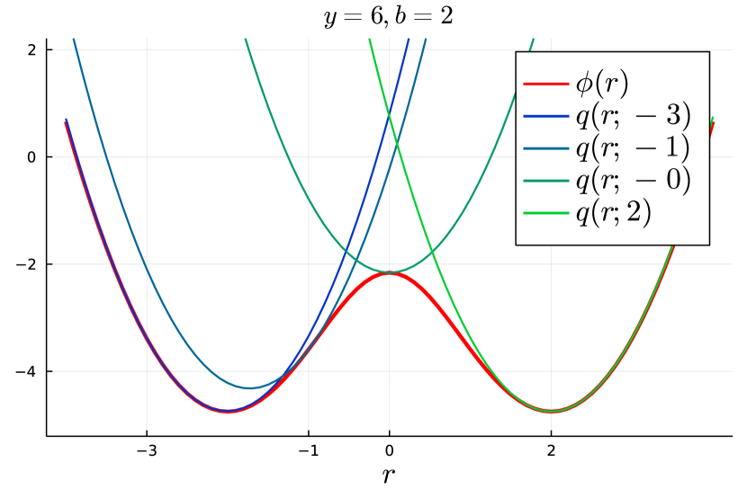
Figure 1: Quadratic majorizers for the non-convex Poisson log-likelihood function $\phi(r;y,b)$ when $y=6$ and $b=2$.

With a bit more work to generalize to $\mathbb{C}^{N}$, a quadratic majorizer for the Poisson ML cost function (7) has the form

$$q(\bm{x};\bm{x}_{k}) \triangleq f(\bm{x}_{k})+(\bm{x}-\bm{x}_{k})^{\prime}\bm{A}^{\prime}\dot{}\bm{\psi}_{\bm{\cdot}}(\bm{A}\bm{x}_{k};\bm{y},{\bm{b}})$$

$$+\frac{1}{2}(\bm{x}-\bm{x}_{k})^{\prime}\bm{A}^{\prime}\bm{W}\bm{A}(\bm{x}-\bm{x}_{k}),$$ (22)

where $\bm{W}$ denotes a diagonal curvature matrix. From (II-A), one choice of $\bm{W}$ uses the maximum of $\ddot{\psi}$:

$$\bm{W}_{\max}\triangleq\operatorname{diag}\{2+\bm{y}/(4{\bm{b}})\}\in\mathbb{R}^{M\times M}.$$ (23)

However, $\bm{W}_{\max}$ is suboptimal because the curvature of a quadratic majorizer of $\psi(v;\cdot)$ varies with $v=[\bm{A}\bm{x}_{k}]_{i}$. For example, when $|v|\rightarrow\infty$, then (7) is dominated by the quadratic term having curvature = 2; so if $y$ is large and $b$ is small, then $\bm{W}_{\max}$ can be much greater than the optimal curvature 2. Thus, instead of using $\bm{W}_{\max}$ to build majorizers, we propose to use the following improved curvature:

$$\bm{W}_{\mathrm{imp}} \triangleq\operatorname{diag}\{\bm{c}_{\bm{\cdot}}(\bm{A}\bm{x}_{k};\bm{y},{\bm{b}})\}\in\mathbb{R}^{M\times M},$$

$$c(s;y,b) \triangleq\left\{\begin{array}[]{ll}\ddot{\psi}\Big{(}\frac{b+\sqrt{b^{2}+b|s|^{2}}}{|s|};y,b\Big{)},&s\neq 0,\\ 2,&s=0.\end{array}\right.$$ (26)

One can verify $\lim_{s\rightarrow 0}c(s;y,b)=2$ so (II-B) is continuous over $s\in\mathbb{C}$. The next subsection proves that (II-B) provides a majorizer in (II-B) and is an improved curvature compared to $\bm{W}_{\max}$, though it is not necessarily the sharpest possible [56]; the sharpest (optimal) curvature $c_{\mathrm{opt}}(s)$ in real case can be expressed as

$$c_{\mathrm{opt}}(s)=\sup_{r\neq s}\frac{2\Big{(}\phi(r)-\phi(s)-\dot{\phi}(s)(r-s)\Big{)}}{(r-s)^{2}},$$ (27)

where $\phi(\cdot)$ is the marginal Poisson cost function defined in (8). However, (27) usually does not have a closed-form solution due to its transcendental derivative; while our $\bm{W}_{\mathrm{imp}}$ has a simpler form and is more efficient to compute. Fig. 2 visualizes the quadratic majorizer with different curvatures and the original Poisson cost function (7). We find the optimal curvature numerically by first discretizing $r$ and then finding the supremum over all discrete segments.

(a)

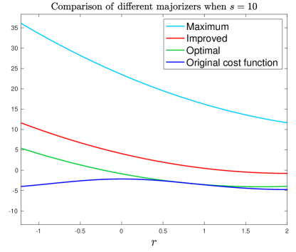
(b)

Figure 2: Comparison of quadratic majorizers with maximum, improved and the optimal curvatures, for $y=6$ and $b=2$, visualized around $r=0.5$. All three curves touch at the point $r=s=10$ by construction.

For the ML case where constraints or regularizers are absent, the quadratic majorizer (II-B) associated with (23) or (II-B) leads to the following MM update:

$$\bm{x}_{k+1} =\operatorname*{arg\,min}_{\bm{x}\in\mathbb{F}^{N}}q(\bm{x};\bm{x}_{k})$$

$$=\bm{x}_{k}-(\bm{A}^{\prime}\bm{W}\bm{A})^{-1}\bm{A}^{\prime}\dot{}\bm{\psi}_{\bm{\cdot}}(\bm{A}\bm{x}_{k};\bm{y},{\bm{b}}).$$ (28)

If $\bm{x}\in\mathbb{R}^{N}$, then the MM update for $\bm{x}_{k+1}$ is

$$\bm{x}_{k}-(\bm{A}^{\prime}\bm{W}\bm{A})^{-1}\mathrm{real}\{\bm{A}^{\prime}\dot{}\bm{\psi}_{\bm{\cdot}}(\bm{A}\bm{x}_{k};\bm{y},{\bm{b}})\}.$$

When $N$ is large, the matrix inverse operation in (II-B) is impractical, so we run a few inner iterations of conjugate gradient (CG) to descend the quadratic majorizer and hence descend the original cost function.

II-B1 Proof of the proposed curvature

For simplicity, we drop the subscript $i$ and irrelevant constants and focus on the negative log-likelihood for real case for simplicity as in (8).

One can generalize the majorizer derived here for (8) to the complex case by taking the magnitude and some other minor modifications.

First, we consider some simple cases:

• If $y=0$, then (8) is a quadratic function, so no quadratic majorizer is needed.

• If $b=0$ and $y>0$ then (8) has unbounded 2nd derivative so no quadratic majorizer exists.

• If $b=0$ and $r=0$, then $y$ must be zero because a Poisson random variable with zero mean can only take the value $0$. Thus again quadratic majorizer is not needed.

So hereafter we assume that $y>0,\ b>0$. Under these assumptions, the derivatives of (8) are:

$$\dot{\phi}(r) =2r\left(1-\frac{y}{r^{2}+b}\right),$$ (29)

$$\ddot{\phi}(r) =2+2y\frac{r^{2}-b}{(r^{2}+b)^{2}},$$ (30)

$$\phi^{(3)}(r) =\frac{2yr(3b-r^{2})}{(r^{2}+b)^{3}},$$ (31)

where $\phi^{(3)}(r)$ denotes the third derivative. Clearly, $\dot{\phi}(r)$ is convex on $(-\infty,-\sqrt{3b}]$ and $[0,\sqrt{3b}]$, and concave on $[-\sqrt{3b},0]$ and $[\sqrt{3b},+\infty)$, based on the sign of $\phi^{(3)}(r)$.

A quadratic majorizer of $\phi(\cdot)$ at point $s$ has the form:

$$\Phi(r;s)=\phi(s)+\dot{\phi}(s)(r-s)+\frac{1}{2}c(s)(r-s)^{2}.$$ (32)

The derivative of this function (w.r.t. $r$) is:

$$\dot{\Phi}(r;s)=c(s)(r-s)+\dot{\phi}(s).$$ (33)

By design, this kind of quadratic majorizer satisfies $\Phi(s;s)=\phi(s)$ and $\dot{\Phi}(s;s)=\dot{\phi}(s)$. From (31), we note that $r^{2}=3b$ is a maximizer of $\ddot{\phi}$ so the maximum curvature is:

$$\ddot{\phi}(r)\leq 2y\frac{2b}{(4b)^{2}}+2=2+\frac{y}{4b}.$$ (34)

Proposition: $\Phi(r;s)$ defined in (32) is a majorizer of $\phi(r)$ when $c(s)=c_{\text{imp}}(s),$ where:

$$c_{\text{imp}}(s)\triangleq\left\{\begin{array}[]{ll}\ddot{\phi}\!\left(u(s)\right),&s\neq 0,\\ \displaystyle\lim_{s\rightarrow 0}\ddot{\phi}\!\left(u(s)\right),&s=0,\end{array}\right.$$ (35)

where

$$u(s)\triangleq\frac{b+\sqrt{b^{2}+bs^{2}}}{s}.$$ (36)

By construction, the proposed curvature $c(s)$ is at most the max curvature given in (34).

Proof: Because of the symmetry of $\ddot{\phi}(r)$, it suffices to prove the proposition for $s\geq 0$ without loss of generality. First we consider some trivial cases:

1. If $s=0$, one can verify $\lim_{s\rightarrow 0}\ddot{\phi}\!\left(u(s)\right)=2$. In this case, $\Phi(r;s)$ is simply

   $$\Phi(r;0) =\phi(0)+\frac{1}{2}c(0)r^{2}$$ (37)

   $$=r^{2}+b-y\log(b)$$

   $$\geq r^{2}+b-y\log(r^{2}+b)=\phi(r).$$

2. If $s=\sqrt{3b}$, one can verify

   $$\ddot{\phi}(g(\sqrt{3b}))=2+\frac{y}{4b},$$ (38)

   which equals the maximum curvature.

Hereafter, we consider only $s>0$ and $s\neq\sqrt{3b}$.

To proceed, it suffices to prove

$$\begin{split}\forall r\in(-\infty,s],\ \dot{\phi}(r)\geq\dot{\Phi}(r;s),\\ \forall r\in[s,+\infty),\ \dot{\phi}(r)\leq\dot{\Phi}(r;s),\end{split}$$ (39)

because if (39) holds, then $\forall\tilde{r}<s$:

$$\Phi(s;s)-\Phi(\tilde{r};s) =\int_{\tilde{r}}^{s}\dot{\Phi}(r;s)dr$$

$$\leq\int_{\tilde{r}}^{s}\dot{\phi}(r)dr=\phi(s)-\phi(\tilde{r}),$$ (40)

and $\forall\tilde{r}>s$:

$$\Phi(\tilde{r};s)-\Phi(s;s) =\int_{s}^{\tilde{r}}\dot{\Phi}(r;s)dr$$

$$\geq\int_{s}^{\tilde{r}}\dot{\phi}(r)dr=\phi(\tilde{r})-\phi(s).$$ (41)

Together with $\Phi(s;s)=\phi(s)$, we have shown that (39) implies $\Phi(r;s)\geq\phi(r),\,\forall r\in\mathbb{R}$.

Substituting $\dot{\Phi}(r;s)=c(s)(r-s)+\dot{\phi}(s)$ into (39), one can verify that showing (39) becomes showing

$$c_{\text{imp}}(s)\geq\frac{\dot{\phi}(r)-\dot{\phi}(s)}{r-s},\quad\forall r\in\mathbb{R},\ r\neq s.$$ (42)

Furthermore, when $s>0$, the parabola $\Phi(\cdot;s)$ is symmetric about its minimizer:

$$\delta =\delta(s)\triangleq\operatorname*{arg\,min}_{r}\ \Phi(r;s)=s-\frac{\dot{\phi}(s)}{c_{\text{imp}}(s)}$$

$$=\frac{s\,\ddot{\phi}(u(s))-\dot{\phi}(s)}{\ddot{\phi}(u(s))}\geq 0.$$ (43)

This minimizer is nonnegative because $\dot{\phi}(s)\leq 2s$ and

$$c_{\text{imp}}(s)=\ddot{\phi}(u(s)) =2+\frac{ys^{2}(b+\sqrt{b^{2}+bs^{2}})}{b(b+s^{2}+\sqrt{b^{2}+bs^{2}})^{2}}$$

$$\geq 2.$$ (44)

Thus, if $\phi(r)\leq\Phi(r;s)$ when $r\geq 0$, we have $\phi(-r)=\phi(r)\leq\Phi(r;s)\leq\Phi(-r;s)=\Phi(r+2\delta;s)$, so it suffices to prove (42) only for $r\geq 0$, which simplifies (42) to showing

$$c_{\text{imp}}(s)\geq\frac{\dot{\phi}(r)-\dot{\phi}(s)}{r-s},\quad\forall r\geq 0,\ r\neq s.$$ (45)

In short, if (45) holds, then $\Phi(r;s)\geq\phi(r),\ \forall r\in\mathbb{R}$.

To prove (45), we exploit a useful property of $c_{\text{imp}}(s)$. Under geometric view, $c_{\text{imp}}(s)$ defines (the ratio of) an affine function connecting points $(u(s),\dot{\phi}(u(s)))$ and $(s,\dot{\phi}(s))$ is tangent to $\dot{\phi}(r)$ at point $r=u(s)$, so that one can verify

$$\ddot{\phi}(u(s))=c_{\text{imp}}(s)=\frac{\dot{\phi}(u(s))-\dot{\phi}(s)}{u(s)-s},\quad u(s)\neq s.$$ (46)

The reason why $u(s)\neq s$ is that one can verify $u(s)=s$ implies $s=\sqrt{3b}$ for $s>0$ that has already been proved above.

Let $\xi(r)=(\dot{\phi}(r)-\dot{\phi}(s))/(r-s)$, where $r\geq 0$ and $r\neq s$, plugging in $\dot{\phi}(r)$ and $\dot{\phi}(s)$ yields:

$$\xi(r)=2+\frac{2y(sr-b)}{(s^{2}+b)(r^{2}+b)}.$$ (47)

Differentiating w.r.t. $r$ leads to:

$$\dot{\xi}(r)=\frac{2y}{s^{2}+b}\cdot\frac{-sr^{2}+2br+bs}{(r^{2}+b)^{2}},$$ (48)

where one can verify the positive root of $-sr^{2}+2br+bs=0$ is $u(s)$ that is given by (36).

Together with $\dot{\xi}(r)>0$ when $r\in(0,u(s))$ and $\dot{\xi}(r)<0$ when $r\in(u(s),\infty)$, we have (45) holds because $\xi(r)$ achieves its maximum at $\xi(u(s))$:

$$\xi(r)\leq\xi(u(s))=c_{\text{imp}}(s).\quad\blacksquare$$ (49)

II-B2 Regularized MM

For the regularized cost function (16), one can use the quadratic majorizer (II-B) as a starting point. If the regularizer is prox-friendly, then the minimization step of an MM algorithm for the regularized optimization problem is

$$\bm{x}_{k+1}=\operatorname*{arg\,min}_{\bm{x}\in\mathbb{F}^{N}}q(\bm{x};\bm{x}_{k})+\beta\|\bm{T}\bm{x}\|_{1}.$$ (50)

To solve (50), one can apply proximal gradient methods [57, 58, 59]. We can use the proximal optimized gradient method (POGM) with adaptive restart [59] that provides faster worst-case convergence bound than the fast iterative shrinkage-thresholding algorithm (FISTA) [58].

For non-proximal friendly regularizers, we can “smooth” it using the Huber function (II-A2), leading to the optimization problem of the form

$$\bm{x}_{k+1}=\operatorname*{arg\,min}_{\bm{x}\in\mathbb{F}^{N}}q(\bm{x};\bm{x}_{k})+\beta 1^{\prime}h_{\bm{\cdot}}(\bm{T}\bm{x};\alpha),$$ (51)

and we use nonlinear CG for this minimization, with step sizes based on Huber’s quadratic majorizer.

Algorithm 2 summarizes our MM algorithm with quadratic majorizer using the improved curvature (II-B).

Input: $\bm{A},\bm{y},{\bm{b}},\bm{x}_{0}$ and $n$ (number of iterations)

for $k=0,...,n-1$ do

      Build $q(\bm{x};\bm{x}_{k})$ (II-B) using $\bm{W}_{\mathrm{imp}}$ (II-B)

      if cost function is regularized then

           if $\bm{T}$ is prox-friendly then

                Update $\bm{x}_{k}$ by (50) using POGM

           else

                Update $\bm{x}_{k}$ by (51) using CG

           end if

          

      else

           Update $\bm{x}_{k}$ by (II-B) or CG

      end if

     

end for

Output: $\bm{x}_{n}$

Algorithm 2 MM algorithm for the Poisson model

III Implementation Details

This section introduces the implementation details of algorithms discussed in the previous section and our experimental setup for the numerical simulation (Section IV). We ran all algorithms on a server with Ubuntu 16.04 LTS operating system having Intel(R) Xeon(R) CPU E5-2698 v4 @ 2.20GHz and 187 GB memory. All elements in the measurement vector $\bm{y}$ were simulated to follow independent Poisson distributions per (6). All algorithms were implemented in Julia v1.7.3. All the timing results presented in Section IV were averaged across 10 independent test runs.

III-A Initialization

Luo et al. [60] proposed the optimal initialization strategy under random Gaussian system matrix setting with Poisson noise. Since this paper focuses on very low-count regimes, the scale factor $\kappa$ in [60] is a very small number so that $y-\kappa\approx y$. Therefore, we used $\tilde{\bm{x}}_{0}$, the leading eigenvector of $\bm{A}^{\prime}\operatorname{diag}\{\bm{y}\varoslash(\bm{y}+1)\}\bm{A}$ (instead of $\bm{A}^{\prime}\operatorname{diag}\{(\bm{y}-\kappa)\varoslash(\bm{y}+1)\}\bm{A}$) as an initial estimate of $\bm{x}$.

To accommodate signals of arbitrary scale, we scaled that leading eigenvector using a nonlinear least-square (LS) fit:

$$\hat{\alpha}=\operatorname*{arg\,min}_{\alpha\in\mathbb{R}}\|\bm{y}-{\bm{b}}-|\alpha\bm{A}\tilde{\bm{x}}_{0}|^{2}\|_{2}^{2}=\frac{\sqrt{(\bm{y}-{\bm{b}})^{\prime}|\bm{A}\tilde{\bm{x}}_{0}|^{2}}}{\|\bm{A}\tilde{\bm{x}}_{0}\|_{4}^{2}}.$$ (52)

Finally, our initial estimate is the element-wise absolute value of $\hat{\alpha}\bm{x}_{0}$ if $\bm{x}$ is known to be real and nonnegative; and is $\hat{\alpha}\bm{x}_{0}$ otherwise.

III-B Ambiguities

To handle the global phase ambiguity, i.e., all the algorithms can recover the signal only to within a constant phase shift due to the loss of global phase information, before quantitative comparison, we corrected the phase of $\hat{\bm{x}}$ by

$$\hat{\bm{x}}_{\textup{corrected}}\triangleq\mathrm{sign}\left(\langle\hat{\bm{x}},\bm{x}\rangle\right)\hat{\bm{x}}.$$ (53)

III-C System matrix and True signals

III-C1 System matrix

We investigated 4 different choices for the system matrix $\bm{A}$: complex random Gaussian matrix (having $80000$ rows), canonical DFT (with reference image), masked DFT matrix (with 20 masks) and a transmission matrix (ETM) that is acquired empirically through physical experiments [61, 62].

For the canonical DFT, we used a reference image as used in holographic coherent diffraction imaging (HCDI) [31], specifically, the measurements follow

$$\bm{y}\sim\textup{Poisson}(|\mathcal{F}\{[\bm{x},\bm{0},\mathcal{R}]\}|^{2}+{\bm{b}}),$$ (54)

where $\mathcal{F}$ denotes discrete Fourier transform (DFT) and $\mathcal{R}$ denotes a known reference image. This paper uses the reference image shown in Fig. 3, taken by screen shot from [31].

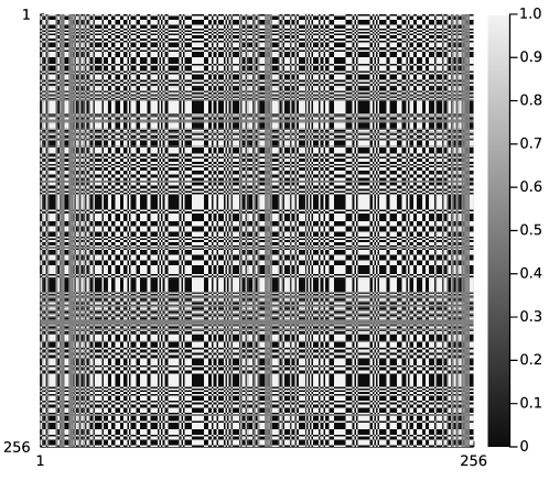
Figure 3: Reference image from [31] used in HCDI and our canonical DFT experiments.

For the masked DFT case, the measurement vector $\bm{y}$ in the Fourier phase retrieval problem has elements with means given by

$$\mathbb{E}[y[\tilde{n}]]=\Bigg{|}\sum_{n=0}^{N-1}x[n]e^{-\imath 2\pi n\tilde{n}/\tilde{N}}\Bigg{|}^{2}+\,b[\tilde{n}],$$ (55)

where $\tilde{N}=2N-1$ (here we consider the over-sampled case), and $\tilde{n}=0,...,\tilde{N}-1$. After introducing redundant masks, the measurement model becomes

$$\mathbb{E}[y_{l}[\tilde{n}]]=\Bigg{|}\sum_{n=0}^{N-1}x[n]D_{l}[n]e^{-\imath 2\pi n\tilde{n}/\tilde{N}}\Bigg{|}^{2}+b_{l}[\tilde{n}],$$ (56)

where $\mathbb{E}[\bm{y}_{l}]\in\mathbb{R}^{\tilde{N}}$ for $i=1,\ldots,L$ and $D_{l}$ denotes the $l$th of $L$ masks. Our experiment used $L=21$ masks to define the overall system matrix $\bm{A}\in\mathbb{C}^{L\tilde{N}\times N}$, where the first mask has full sampling and the remaining 20 have sampling rate 0.5 with random sampling patterns.

We scaled each system matrix by a constant factor such that the average count of measurement vector $\bm{y}$ is 0.25, and the background count $b$ is set to be 0.1.

III-C2 True images

We considered 4 images as the true images in our experiments Fig. 4 shows such images; (b) is from [63], (c) is from [31], (d)-(f) are from [62]. We used subfigure (a) for experiments with random Gaussian system matrix, (b) for masked DFT matrix, (c) for canonical DFT matrix and (d) for empirical transmission matrix, respectively.

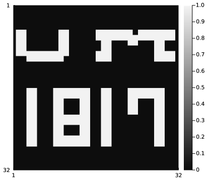
(a)

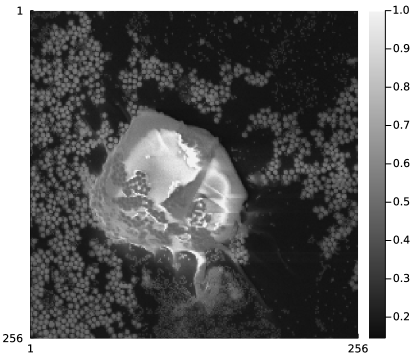
(b)

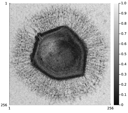
(c)

(d)

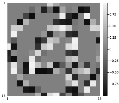
(e)

(f)

Figure 4: True images used in the simulations. Subfigure (d) shows the magnitude of a complex image.

IV Numerical Simulations Results

IV-A Convergence speed of WF with Fisher information

This section compares convergence speeds, in terms of cost function vs. time and PSNR vs. time, between WF using our proposed Fisher information for step size, and empirical step size [15], backtracking line search [21], the optimal step size for the Gaussian ML cost function [18], and LBFGS quasi-Newton to approximate the Hessian in Newton’s method [26]. The LBFGS algorithm was from the “Optim.jl” Julia package [64].

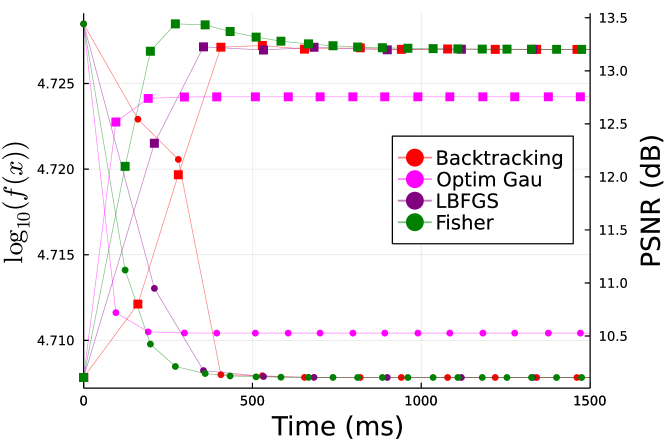
(a)

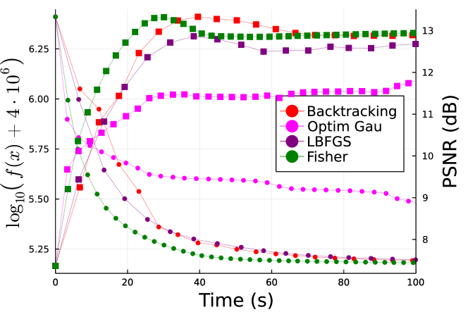
(b)

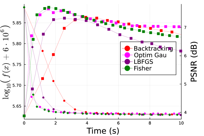
(c)

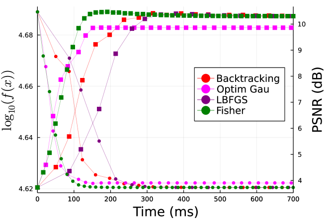
(d)

Figure 5: Comparison of convergence speed for various WF methods and LBFGS under different system matrix settings. The “Optim Gau” curve is WF using the curvature from [18] that is optimal for Gaussian noise. The circle marker corresponds to the cost function and the square marker corresponds to PSNR.

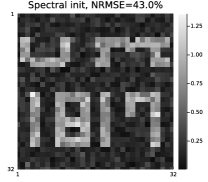
(a)

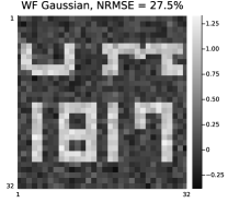
(b)

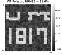
(c)

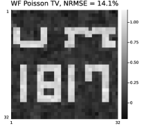
(d)

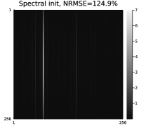
(e)

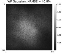
(f)

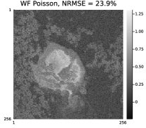
(g)

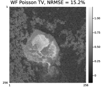
(h)

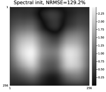
(i)

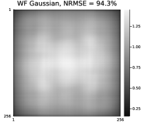
(j)

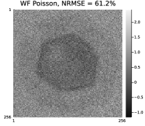
(k)

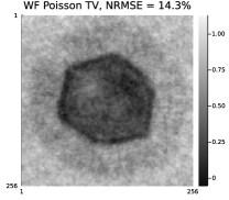
(l)

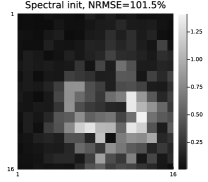
(m)

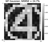
(n)

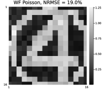
(o)

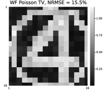
(p)

Figure 6: Reconstruction quality comparison between four methods (left to right): the optimal Poisson spectral initialization [60], the WF Gaussian method, the WF Poisson method, and WF Poisson with TV regularization. System matrices: (a)-(d) random Gaussian; (e)-(h) masked DFT; (i)-(l) canonical DFT with reference image; (m)-(p) ETM. Magnitude of complex images shown. All WF algorithms used the proposed Fisher information for step size.

Fig. 5 shows that, for all system matrix choices, WF with Fisher information converged faster (in terms of decreasing the cost function) than all other methods; the LBFGS algorithm had comparable convergence speed as WF with backtracking line search. We found that WF with the empirical step size did not converge using hyper-parameters in [15] so we excluded those results in Fig. 5. The backtracking approach, although slower than Fisher approach per wall-time, is faster per-iteration. However, the step size found by backtracking line search could be sensitive to hyper-parameter choices. For the WF algorithm with optimal step size (derived based on Gaussian noise model [18]), we conjectured that it reached a non-stationary point that has larger cost function value than those of other methods, as expected.

In terms of PSNR, we found that in random Gaussian, masked DFT and empirical transmission cases, WF with Fisher information increased the PSNR faster than all other methods; WF with optimal Gaussian step size led to lower PSNR, perhaps again due to reaching a sub-optimal minimizer. However, for the canonical Fourier case, we found that all methods started decreasing PSNR after several iterations. The algorithms may be more sensitive to noise in the canonical Fourier matrix setting, especially in the very low-count regime considered here. Apparently WF with optimal Gaussian step size overfits the noise more slowly due to its sub-optimal step size under Poisson noise.

IV-B Comparison of Poisson and Gaussian algorithms

This section compares the reconstruction quality, i.e., the NRMSE to the true signal, between WF derived from the Gaussian ML cost function (3), and WF derived from the Poisson ML cost function (7) as well as regularized WF under different system matrix settings. We used corner-rounded TV regularizer with $\beta=32$ and $\alpha=0.1$ in the regularized WF algorithm.

Fig. 6 shows that algorithms derived from the Poisson model yielded consistently better reconstruction quality (lower NRMSE) than algorithms derived from the Gaussian model, as expected. Furthermore, by incorporating regularizer that exploits the assumed property of the true signal, the NRMSE was further decreased. Spectral initialization worked well in random Gaussian matrix setting, but not for other system matrices, as expected from its theory. The WF Gaussian approach failed to reconstruct in masked and canonical DFT system matrix setting. Since incorporating appropriate regularizers helps algorithms yield higher quality reconstructions, a question is naturally raised about which regularized algorithm converges the fastest. The next subsection presents such comparisons.

IV-C Convergence speed of regularized Poisson algorithms

As discussed in Section II, many algorithms can be modified to accommodate regularizers. We compared the convergence speeds of regularized Poisson algorithms (WF Fisher, WF backtracking, LBFGS, MM and ADMM [46]), with a smooth regularizer (corner-rounded TV), under different system matrix settings. Based on Fig. 5, we did not run simulations of regularized WF with empirical step size and with Gaussian optimal step size, due to their non-converging trend and sub-optimal solution, respectively. For all other algorithms, we set the regularization parameters to be $\beta=32$ and $\alpha=0.1$ (defined in (16) and (II-A2)).

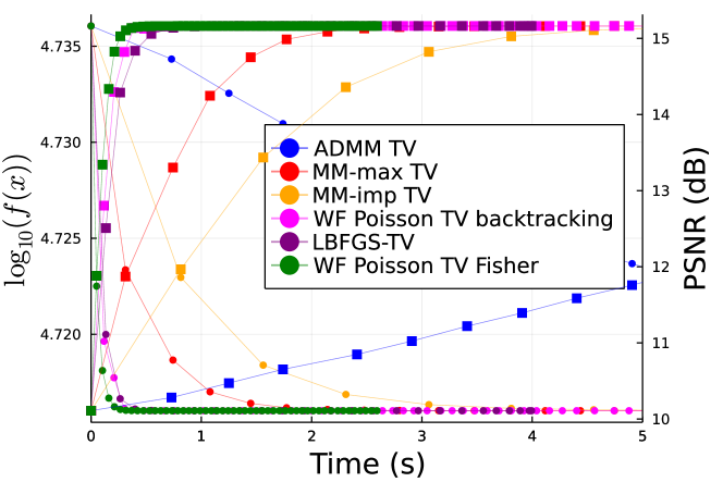
(a)

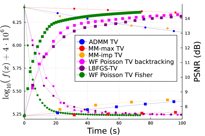
(b)

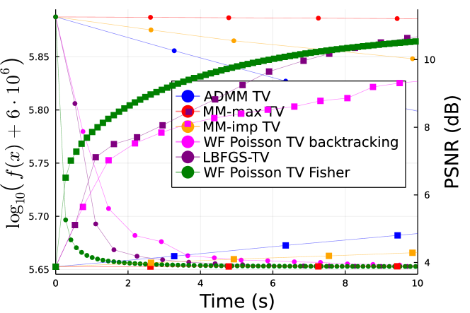
(c)

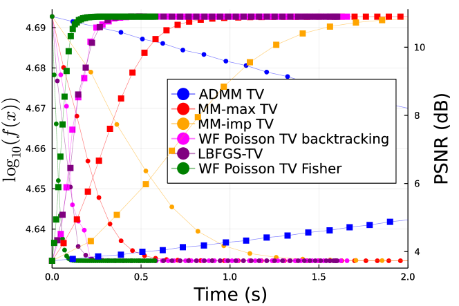
(d)

Figure 7: Comparison of convergence speed of variant algorithms with corner-rounded TV regularizer. The circle marker corresponds to cost function and the square marker corresponds to PSNR.

Fig. 7 shows that the regularized WF with our proposed Fisher information for step size converged the fastest compared to other methods under all different system matrices. The LBFGS again had a comparable convergence speed as WF using backtracking line search. The MM algorithm with improved curvature, was slower in wall-time due to extra computation per iteration, but was faster per iteration due to its sharper curvature. In masked and canonical Fourier case, however, MM with improved curvature was faster than the maximum curvature in wall-time comparison, which can be attributed to large magnitude low frequency components in the coefficients of the Fourier transform.

V Discussion

Current methods for phase retrieval mostly focus on ML estimation for Gaussian noise; fewer algorithms were derived for Poisson noise [36, 6, 43]. Here we proposed a novel WF algorithm and an MM algorithm and then did an empirical study on the convergence speed as well as reconstruction quality of several Poisson phase retrieval algorithms. In our proposed WF algorithm, we first replaced the gradient term in Gaussian WF (4) with its Poisson counterpart (II-A). Then we did a quadratic approximation of the cost function and applied one iteration of Newton’s method to define an “optimal” step size. We then proposed to use the observed Fisher information to approximate the Hessian when computing the step size, which is a common method in computational statistics. Moreover, the Fisher information matrix is guaranteed to be positive semi-definite and is more computationally efficient compared to the Hessian. To further illustrate our proposed method of using Fisher information to approximate the Hessian, Fig. 8 visualizes these two matrices (in marginal forms).

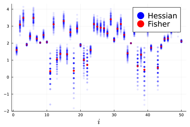
Figure 8: Visualization of the marginal Hessian (II-A) and the marginal observed Fisher information (II-A1). The horizontal axis denotes the $i$th element in the marginal Hessian/Fisher. Data were simulated with a random Gaussian matrix and 100 independent realizations.

As shown in Fig. 8, the Hessian is noisy and can have some negative elements. Such undesirable features can lead to unstable step size calculations. In contrast, the elements in Fisher information matrix are non-negative and less noisy. We ran some experiments and found that when the background counts $b_{i}$ are large, using the noisy Hessian to calculate the step size can lead to divergence of the cost function, due to the negative values in the marginal second derivative. Setting such negative values in the second derivative to zero is a possible solution, but we found that approach led to slower convergence than using the Fisher information. One potential alternative to our approach is to use the empirical Fisher information, but that may be suboptimal since the empirical Fisher information does not generally capture second-order information [65].

To accommodate our WF algorithm with non-smooth regularizers, e.g., $\|\bm{T}\bm{x}\|_{1}$, we used a Huber function to approximate the $\ell_{1}$ norm with a quadratic function around zero, so that the Wirtinger gradient is well-defined everywhere. A limitation of this paper is that we did not consider other regularizers in our experiments, though our algorithms can be generalized to handle other smooth regularizers with minor modifications. One drawback of TV regularization is that it assumes piece-wise uniform latent images so it lacks generalizability to other kinds of images, One way to address this is to train deep neural networks [66, 67] with a variety of images, potentially leading to better generalizability.

VI Conclusion

This paper proposed and compared algorithms based on ML estimation and regularized ML estimation for phase retrieval from Poisson measurements, in very low-photon count regimes, e.g., 0.25 photon per pixel. We proposed a novel method that used the Fisher information to compute the step size in the WF algorithm; this approach eliminates all parameter tuning except the number of iterations. We also proposed a novel MM algorithm with improved curvature compared to the one derived from the upper bound of the second derivative of the cost function.

Simulation results experimented on random Gaussian matrix, masked DFT matrix, canonical DFT matrix and an empirical transmission matrix showed that: 1) For unregularized algorithms, the WF algorithm using our proposed Fisher information for step size converged faster than using empirical step size, backtracking line search, optimal step size for Gaussian noise model and LBFGS. Moreover, our proposed Fisher step size can be computed efficiently without any tuning parameter. 2) As expected, algorithms derived from the Poisson noise model produce consistently better reconstruction quality than algorithms derived from the Gaussian noise model for low-count data. Furthermore, by incorporating regularizers that exploit the assumed properties of the true signal, the reconstruction quality can be further improved. 3) For regularized algorithms with smooth corner-rounded TV regularizer, WF with Fisher information converges faster than WF with backtracking line search, LBFGS, MM and ADMM.

Future work includes precomputing and tabluting the optimal curvature for the quadratic majorizer, establishing sufficient conditions for global convergence, investigating algorithms with other kind of regularizers (e.g., deep learning methods [66, 67]), investigating sketching methods for large problem sizes [68], and testing Poisson phase retrieval algorithms under a wider variety of experimental settings.

References

References

- [1] K. Jaganathan, Y.. Eldar and B. Hassibi “Phase retrieval: an overview of recent developments” https://arxiv.org/abs/1510.07713, 2015
- [2] P. Grohs, S. Koppensteiner and M. Rathmair “Phase retrieval: uniqueness and stability” In SIAM Review 62.2, 2020, pp. 301–50 DOI: 10.1137/19M1256865
- [3] P. Jaming “Phase retrieval techniques for radar ambiguity problems.” In J. Four. Anal. Appl. 5.4, 1999, pp. 309–329
- [4] R.. Millane “Phase retrieval in crystallography and optics” In J. Opt. Soc. Am. A 7.3, 1990, pp. 394–411 DOI: 10.1364/JOSAA.7.000394
- [5] J. Dainty and James Fienup “Phase retrieval and image reconstruction for astronomy” In Imag. Recov. Theory Appl. 13, 1987, pp. 231–275
- [6] L. Bian, J. Suo, J. Chung, X. Ou, C. Yang, F. Chen and Q. Dai “Fourier ptychographic reconstruction using Poisson maximum likelihood and truncated Wirtinger gradient” In Nature Sci. Rep. 6.1, 2016 DOI: 10.1038/srep27384
- [7] Y. Zhang, P. Song and Q. Dai “Fourier ptychographic microscopy using a generalized Anscombe transform approximation of the mixed Poisson-Gaussian likelihood” In Optics Express 25.1, 2017, pp. 168–79 DOI: 10.1364/OE.25.000168
- [8] Rui Xu, Mahdi Soltanolkotabi, Justin P. Haldar, Walter Unglaub, Joshua Zusman, Anthony F.. Levi and Richard M. Leahy “Accelerated Wirtinger Flow: A fast algorithm for ptychography” http://arxiv.org/abs/1806.05546, 2018 arXiv:1806.05546 [eess.IV]
- [9] X. Tian “Fourier ptychographic reconstruction using mixed Gaussian-Poisson likelihood with total variation regularisation” In Electronics Letters 55.19, 2019, pp. 1041–3 DOI: 10.1049/el.2019.1141
- [10] Tatiana Latychevskaia “Iterative phase retrieval in coherent diffractive imaging: practical issues” In Appl. Opt. 57.25 Optica Publishing Group, 2018, pp. 7187–7197 DOI: 10.1364/AO.57.007187
- [11] D.. Snyder, C.. Helstrom, A.. Lanterman, M. Faisal and R.. White “Compensation for readout noise in CCD images” In J. Opt. Soc. Am. A 12.2, 1995, pp. 272–83 DOI: 10.1364/JOSAA.12.000272
- [12] Emmanuel J Candès, Thomas Strohmer and Vladislav Voroninski “PhaseLift: Exact and Stable Signal Recovery from Magnitude Measurements via Convex Programming” In Comm. Pure Appl. Math. 66.8 Hoboken: Wiley Subscription Services, Inc., A Wiley Company, 2013, pp. 1241–1274 DOI: 10.1002/cpa.21432
- [13] Afonso S Bandeira, Jameson Cahill, Dustin G Mixon and Aaron A Nelson “Saving phase: Injectivity and stability for phase retrieval” In Appl. Comp. Harm. Anal. 37.1 Elsevier Inc, 2014, pp. 106–125 DOI: 10.1016/j.acha.2013.10.002
- [14] Afonso S Bandeira, Yutong Chen and Dustin G Mixon “Phase retrieval from power spectra of masked signals” In Info. Infer. 3.2 Oxford University Press, 2014, pp. 83–102 DOI: 10.1093/imaiai/iau002
- [15] E.. Candes, Y.. Eldar, T. Strohmer and V. Voroninski “Phase retrieval via matrix completion” In SIAM J. Imaging Sci. 6.1, 2013, pp. 199–225 DOI: 10.1137/110848074
- [16] Yoav Shechtman, Yonina C Eldar, Oren Cohen, Henry Nicholas Chapman, Jianwei Miao and Mordechai Segev “Phase Retrieval with Application to Optical Imaging: A contemporary overview” In IEEE Sig. Proc. Mag. 32.3 IEEE, 2015, pp. 87–109 DOI: 10.1109/MSP.2014.2352673
- [17] Emmanuel Candes, Xiaodong Li and Mahdi Soltanolkotabi “Phase Retrieval via Wirtinger Flow: Theory and Algorithms” In IEEE Trans. Info. Theory 61.4, 2015, pp. 1985–2007 DOI: 10.1109/TIT.2015.2399924
- [18] Xue Jiang, Sreeraman Rajan and Xingzhao Liu “Wirtinger Flow Method With Optimal Stepsize for Phase Retrieval” In IEEE Sig. Proc. Letters 23.11 IEEE, 2016, pp. 1627–1631 DOI: 10.1109/LSP.2016.2611940
- [19] T. Cai, Xiaodong Li and Zongming Ma “Optimal Rates of Convergence for Noisy Sparse Phase Retrieval via Thresholded Wirtinger Flow” In Annals Stat. 44.5 Hayward: Institute of Mathematical Statistics, 2016, pp. 2221–2251 DOI: 10.1214/16-AOS1443
- [20] Mahdi Soltanolkotabi “Structured Signal Recovery From Quadratic Measurements: Breaking Sample Complexity Barriers via Nonconvex Optimization” In IEEE Trans. Info. Theory 65.4 IEEE, 2019, pp. 2374–2400 DOI: 10.1109/TIT.2019.2891653
- [21] T. Qiu, P. Babu and D.. Palomar “PRIME: phase retrieval via majorization-minimization” In IEEE Trans. Sig. Proc. 64.19, 2016, pp. 5174–86 DOI: 10.1109/TSP.2016.2585084
- [22] R.. Gerchberg and W.. Saxton “Practical Algorithm for Determination of Phase from Image and Diffraction Plane Pictures” In OPTIK 35.2, 1972, pp. 237–246
- [23] Praneeth Netrapalli, Prateek Jain and Sujay Sanghavi “Phase Retrieval Using Alternating Minimization” In IEEE Trans. Sig. Proc. 63.18 IEEE, 2015, pp. 4814–4826 DOI: 10.1109/TSP.2015.2448516
- [24] Irene Waldspurger “Phase Retrieval With Random Gaussian Sensing Vectors by Alternating Projections” In IEEE Trans. Info. Theory 64.5 IEEE, 2018, pp. 3301–3312 DOI: 10.1109/TIT.2018.2800663
- [25] Bing Gao and Zhiqiang Xu “Phaseless Recovery Using the Gauss-Newton Method” In IEEE Trans. Sig. Proc. 65.22 IEEE, 2017, pp. 5885–5896 DOI: 10.1109/TSP.2017.2742981
- [26] Li Ji and Zhou Tie “On gradient descent algorithm for generalized phase retrieval problem” In 2016 IEEE 13th International Conference on Signal Processing (ICSP) IEEE, 2016, pp. 320–325 DOI: 10.1109/ICSP.2016.7877848
- [27] Junli Liang, Petre Stoica, Yang Jing and Jian Li “Phase Retrieval via the Alternating Direction Method of Multipliers” In IEEE Sig. Proc. Letters 25.1, 2018, pp. 5–9 DOI: 10.1109/LSP.2017.2767826
- [28] Yang Yang, Marius Pesavento, Yonina C. Eldar and Björn Ottersten “Parallel Coordinate Descent Algorithms for Sparse Phase Retrieval” In ICASSP 2019 - 2019 IEEE International Conference on Acoustics, Speech and Signal Processing (ICASSP), 2019, pp. 7670–7674 DOI: 10.1109/ICASSP.2019.8683363
- [29] P. Thibault and M. Guizar-Sicairos “Maximum-likelihood refinement for coherent diffractive imaging” In New J. of Phys. 14.6, 2012, pp. 063004 DOI: 10.1088/1367-2630/14/6/063004
- [30] A. Goy, K. Arthur, S. Li and G. Barbastathis “Low photon count phase retrieval using deep learning” In Phys. Rev. Lett. 121.24, 2018, pp. 243902 DOI: 10.1103/PhysRevLett.121.243902
- [31] David A. Barmherzig and Ju Sun “Low-Photon Holographie Phase Retrieval” In Imaging and Applied Optics Congress Optica Publishing Group, 2020 DOI: 10.1364/COSI.2020.JTu4A.6
- [32] I. Vazquez, I.. Harmon, J… Luna and M. Das “Quantitative phase retrieval with low photon counts using an energy resolving quantum detector” In J. Opt. Soc. Am. A 38.1, 2021, pp. 71–9 DOI: 10.1364/JOSAA.396717
- [33] H. Lawrence, D.. Barmherzig, H. Li, M. Eickenberg and M. Gabrie “Phase retrieval with holography and untrained priors: Tackling the challenges of low-photon nanoscale imaging” http://arxiv.org/abs/2012.07386, 2020
- [34] Abhiram Gnanasambandam and Stanley H. Chan “Image Classification in the Dark using Quanta Image Sensors” https://arxiv.org/abs/2006.02026, 2020 arXiv:2006.02026 [eess.IV]
- [35] K. Choi and A.. Lanterman “Phase retrieval from noisy data based on minimization of penalized I-divergence” In J. Opt. Soc. Am. A 24.1, 2007, pp. 34–49 DOI: 10.1364/JOSAA.24.000034
- [36] Y. Chen and E.. Candes “Solving random quadratic systems of equations is nearly as easy as solving linear systems” In Comm. Pure Appl. Math. 70.5, 2017, pp. 822–83 DOI: 10.1002/cpa.21638
- [37] H. Chang and S. Marchesini “Denoising Poisson phaseless measurements via orthogonal dictionary learning” In Optics Express 26.16, 2018, pp. 19773–96 DOI: 10.1364/OE.26.019773
- [38] I. Kang, F. Zhang and G. Barbastathis “Phase extraction neural network (PhENN) with coherent modulation imaging (CMI) for phase retrieval at low photon counts” In Optics Express 28.15, 2020, pp. 21578–600 DOI: 10.1364/OE.397430
- [39] D.. Snyder, A.. Hammoud and R.. White “Image recovery from data acquired with a charge-coupled-device camera” In J. Opt. Soc. Am. A 10.5, 1993, pp. 1014–23 DOI: 10.1364/JOSAA.10.001014
- [40] Markku Makitalo and Alessandro Foi “Optimal Inversion of the Generalized Anscombe Transformation for Poisson-Gaussian Noise” In IEEE Trans. Imag. Proc. 22.1, 2013, pp. 91–103 DOI: 10.1109/TIP.2012.2202675
- [41] Ghania Fatima and Prabhu Babu “PGPAL: A monotonic iterative algorithm for Phase-Retrieval under the presence of Poisson-Gaussian noise” In IEEE Sig. Proc. Letters, 2022, pp. 1–1 DOI: 10.1109/LSP.2022.3143469
- [42] H. Zhang, Y. Liang and Y. Chi “A nonconvex approach for phase retrieval: Reshaped Wirtinger flow and incremental algorithms” In J. Mach. Learning Res. 18.141, 2017, pp. 1–35 URL: http://jmlr.org/papers/v18/16-572.html
- [43] Huibin Chang, Yifei Lou, Yuping Duan and Stefano Marchesini “Total variation–based phase retrieval for Poisson noise removal” In SIAM J. Imag. Sci. 11.1 SIAM PUBLICATIONS, 2018, pp. 24–55 DOI: 10.1137/16M1103270
- [44] Ghania Fatima, Zongyu Li, Aakash Arora and Prabhu Babu “PDMM: A novel Primal-Dual Majorization-Minimization algorithm for Poisson Phase-Retrieval problem” In IEEE Trans. Sig. Proc., 2022, pp. 1–1 DOI: 10.1109/TSP.2022.3156014
- [45] Zongyu Li, Kenneth Lange and Jeffrey A. Fessler “Poisson Phase Retrieval With Wirtinger Flow” In 2021 IEEE International Conference on Image Processing (ICIP), 2021, pp. 2828–2832 DOI: 10.1109/ICIP42928.2021.9506139
- [46] Zongyu Li, Kenneth Lange and Jeffrey A. Fessler “Algorithms for Poisson Phase Retrieval” https://arxiv.org/abs/2104.00861, 2021 arXiv:2104.00861
- [47] H. Zhang and D.. Mandic “Is a complex-valued stepsize advantageous in complex-valued gradient learning algorithms?” In IEEE Trans. Neural Net. Learn. Sys. 27.12, 2016, pp. 2730–5 DOI: 10.1109/TNNLS.2015.2494361
- [48] D.. Titterington “Recursive parameter estimation using incomplete data” In J. Royal Stat. Soc. Ser. B 46.2, 1984, pp. 257–67 URL: http://www.jstor.org/stable/2345509
- [49] K. Lange “A gradient algorithm locally equivalent to the EM Algorithm” In J. Royal Stat. Soc. Ser. B 57.2, 1995, pp. 425–37 URL: http://www.jstor.org/stable/2345971
- [50] Lingyao Meng “Method for Computation of the Fisher Information Matrix in the Expectation-Maximization Algorithm” arXiv, 2016 DOI: 10.48550/ARXIV.1608.01734
- [51] M.. Osborne “Fisher’s Method of Scoring” In International Statistical Review 60.1 [Wiley, International Statistical Institute (ISI)], 1992, pp. 99–117 URL: http://www.jstor.org/stable/1403504
- [52] HM. Hudson and J. Ma “Fisher’s method of scoring in statistical image reconstruction: comparison of Jacobi and Gauss-Seidel iterative schemes” In Statistical Methods in Medical Research 3.1, 1994, pp. 41–61 DOI: 10.1177/096228029400300104
- [53] P.. Huber “Robust statistics” New York: Wiley, 1981
- [54] D.. Hunter and K. Lange “A tutorial on MM algorithms” In American Statistician 58.1, 2004, pp. 30–7 DOI: 10.1198/0003130042836
- [55] D. Böhning and B.. Lindsay “Monotonicity of quadratic approximation algorithms” In Ann. Inst. Stat. Math. 40.4, 1988, pp. 641–63 DOI: 10.1007/BF00049423
- [56] J. de Leeuw and K. Lange “Sharp quadratic majorization in one dimension” In Comp. Stat. Data Anal. 53.7, 2009, pp. 2471–84 DOI: 10.1016/j.csda.2009.01.002
- [57] I. Daubechies, M. Defrise and C. De Mol “An iterative thresholding algorithm for linear inverse problems with a sparsity constraint” In Comm. Pure Appl. Math. 57.11, 2004, pp. 1413–57 DOI: 10.1002/cpa.20042
- [58] A. Beck and M. Teboulle “A fast iterative shrinkage-thresholding algorithm for linear inverse problems” In SIAM J. Imaging Sci. 2.1, 2009, pp. 183–202 DOI: 10.1137/080716542
- [59] D. Kim and J.. Fessler “Adaptive restart of the optimized gradient method for convex optimization” In J. Optim. Theory Appl. 178.1, 2018, pp. 240–63 DOI: 10.1007/s10957-018-1287-4
- [60] Wangyu Luo, Wael Alghamdi and Yue M Lu “Optimal Spectral Initialization for Signal Recovery With Applications to Phase Retrieval” In IEEE Trans. Sig. Proc. 67.9 IEEE, 2019, pp. 2347–2356 DOI: 10.1109/TSP.2019.2904918
- [61] Rohan Chandra, Ziyuan Zhong, Justin Hontz, Val McCulloch, Christoph Studer and Tom Goldstein “PhasePack: A Phase Retrieval Library” In Asil. Conf. Sig. Sys. Comp., 2017, pp. 1617–1621
- [62] C.. Metzler, M.. Sharma, S. Nagesh, R.. Baraniuk, O. Cossairt and A. Veeraraghavan “Coherent inverse scattering via transmission matrices: Efficient phase retrieval algorithms and a public dataset” In Proc. Intl. Conf. Comp. Photography, 2017, pp. 1–16 DOI: 10.1109/ICCPHOT.2017.7951483
- [63] Stefano Marchesini “Ptychography Gold Ball Example Dataset”, 2017 DOI: 10.11577/1454414
- [64] P.. Mogensen and Asbjørn Nilsen Riseth “Optim: A mathematical optimization package for Julia” In J. of Open Source Software 3.24, 2018, pp. 615 DOI: 10.21105/joss.00615
- [65] Frederik Kunstner, Philipp Hennig and Lukas Balles “Limitations of the empirical Fisher approximation for natural gradient descent” In Adv. Neural Info. Proc. Sys. 32, 2019
- [66] Tal Remez, Or Litany, Raja Giryes and Alex M. Bronstein “Class-Aware Fully Convolutional Gaussian and Poisson Denoising” In IEEE Trans. Image Proc. 27.11, 2018, pp. 5707–5722 DOI: 10.1109/TIP.2018.2859044
- [67] Zhiyuan Zha, Bihan Wen, Xin Yuan, Jiantao Zhou and Ce Zhu “Simultaneous Nonlocal Low-Rank And Deep Priors For Poisson Denoising” In ICASSP 2022 - 2022 IEEE International Conference on Acoustics, Speech and Signal Processing (ICASSP), 2022, pp. 2320–2324 DOI: 10.1109/ICASSP43922.2022.9746870
- [68] Y. Luo, W. Huang, X. Li and A.. Zhang “Recursive importance sketching for rank constrained least squares: algorithms and high-order convergence”, 2022 URL: http://arxiv.org/abs/2011.08360