Bridging Global Context Interactions for High-Fidelity Image Completion

Abstract

Bridging global context interactions correctly is important for high-fidelity image completion with large masks. Previous methods attempting this via deep or large receptive field (RF) convolutions cannot escape from the dominance of nearby interactions, which may be inferior. In this paper, we propose to treat image completion as a directionless sequence-to-sequence prediction task, and deploy a transformer to directly capture long-range dependence in the encoder. Crucially, we employ a restrictive CNN with small and non-overlapping RF for weighted token representation, which allows the transformer to explicitly model the long-range visible context relations with equal importance in all layers, without implicitly confounding neighboring tokens when larger RFs are used. To improve appearance consistency between visible and generated regions, a novel attention-aware layer (AAL) is introduced to better exploit distantly related high-frequency features. Overall, extensive experiments demonstrate superior performance compared to state-of-the-art methods on several datasets. Code is available at https://github.com/lyndonzheng/TFill.

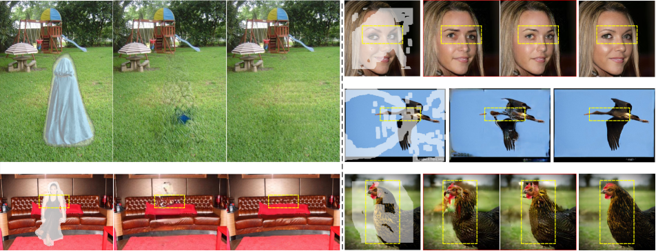
Figure 1: Example completion results of our method on different sceneries with various masks (missing regions shown in white, a transparency ratio is set for better visualization). Our TFill model not only effectively removes large objects (left), but also infers reasonable contents and plausible appearances for semantical image completion on various settings (right). (Zoom in to see the details.)

1 Introduction

Image completion refers to the task of filling reasonable content with photorealistic appearance into missing regions, conditioned on partially visible information (as shown in Fig. 1). Earlier methods infer the pixels of missing regions by propagating pieces from neighboring visible regions [3, 1, 9, 2], while more recent ones directly learn to generate content and appearance using deep neural networks [36, 17, 51, 28, 58, 29, 35, 50, 37, 53, 46].

A main challenge in this task is the requirement of bridging and exploiting visible information globally, after it had been degraded by arbitrary masks. As depicted on the left of Fig. 1, when the entire person is masked, the natural expectation is to complete the masked area based on the visible background context. In contrast, on the right of Fig. 1, when large free-form irregular masks cover the main parts but leave the partial information visible, it is necessary but highly challenging to correctly capture long-range dependencies between the separated foreground regions, so that the masked area can be completed in not just a photorealistic, but also semantically correct, manner.

To achieve this goal, several two-stage approaches [51, 35, 50, 37, 53] have been proposed, consisting of a content inference network and an appearance refinement network. They typically infer a coarse image/edge/semantic map based on globally visible context in a first phase, and then fill in visually realistic appearance in a second phase. However, this global perception is achieved by repeating local convolutional operations, which have several limitations. First, due to the translation equivariance, the information flow tends to be predominantly local, with global information only shared gradually through heat-like propagation across multiple layers. Second, during inference, the elements between adjacent layers are connected via learned but fixed weights, rather than input-dependent adaptive weightings. These issues mean long-distance messages are only delivered inefficiently in a very deep layer, resulting in a strong inclination for the network to fill holes based on nearby rather than distant visible pixels (cf. Fig. 1).

In this paper, we propose an alternative perspective by treating image completion as a directionless sequence-to-sequence prediction task. In particular, instead of modeling the global context using deeply stacked convolutional layers, we design a new content inference model, called TFill, that uses a Transformer-based architecture to Fill reasonable content into the missing holes. An important insight here is that a transformer directly exploits long-range dependencies at every encoder layer through the attention mechanism, which creates an equal flowing opportunity for all visible pixels, regardless of their relative spatial positions (Fig. 4 (c)). This reduces the proximity-dominant influence that can lead to semantically incoherent results.

However, it remains a challenge to directly apply these transformer models to visual generation tasks. In particular, unlike in NLP where each word is naturally treated as a vector for token embedding [45, 10, 39, 40], it is unclear what a good token representation should be for a visual task. If we use every pixel as a token, the memory cost will make this infeasible except for very small downsampled images [8, 46]. To mitigate this issue, our model embeds the masked image into an intermediate latent space for token representation, an approach also broadly taken by recent vision transformer models [6, 62, 12, 60, 48]. However, unlike these models that use traditional CNN-based encoders to embed the tokens, without considering the visible information flow in image completion, we propose a restrictive CNN for token representation, which has a profound influence on how the visible information is connected in the network. To do so, we ensure the individual tokens represent visible information independently, each within a small and non-overlapping patch. This forces the long-range context relationships between tokens to be explicitly and co-equally perceived in every transformer encoder layer, without neighboring tokens being entangled by implicit correlation through overlapping RF. As a result, each masked pixel will not be gradually affected by neighboring visible pixels.

While the proposed transformer-based architecture can achieve better results than state-of-the-art methods [51, 58, 50, 12], by itself it only works for a fixed sequence length because of the position embedding (Fig. 2(a)). To allow our approach to flexibly scale to images of arbitrary sizes, especially at high resolution, a fully convolutional network (Fig. 2(b)) is subsequently applied to refine the visual appearance, building upon the coarse content previously inferred. A novel Attention-Aware Layer (AAL) is inserted between the encoder and decoder that adaptively balances the attention paid to visible and generated content, leading to semantically superior feature transfer (Figs. 5 and 9).

We highlight our main contributions as follows: 1) A restrictive CNN head is introduced for individual weighted token representation, which mitigates the proximity influence when propagating from local visible regions to missing holes. 2) Through a transformer-based architecture, the long-range interactions between these tokens are explicitly modeled, in which the masked tokens are perceptive of other visible tokens with equal opportunity, regardless of their positions. This results in a significant improvement over state-of-the-art methods. 3) A novel attention-aware layer with adaptive attention balancing is introduced in a refined stage to obtain higher quality and resolution results. 4) Finally, extensive experiments demonstrate that the proposed model outperforms the existing state-of-the-art image completion models.

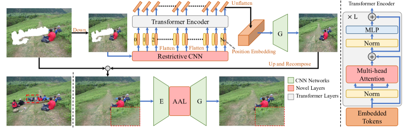
Figure 2: The overall pipeline of our proposed method (The LightPink boxes highlight our designed novel layers). (a) Masked input is resized to a fixed low resolution ($256\times 256$) and it is then fed into a transformer encoder to generate semantically correct content. (b) The inferred content is merged with the original high-resolution image and passed to a refinement network with an Attention-Aware Layer (AAL) to transfer high-quality information from both visible and generated regions. Note the recomposed input has repeating artifacts, which are resolved in our refined network. Zoom in to see the details.

2 Related Work

Image Completion:

Traditional image completion (also known as “image inpainting” [3]) methods, like diffusion-based [1, 26, 4] and patch-based [9, 18, 2], mainly focus on background completion, by directly copying and propagating the background pixels to masked regions.

Driven by the advances of GANs [13], CGANs [34] and VAEs [25], a series of CNN-based methods [36, 17, 51, 28, 58, 35] have been proposed to hallucinate semantic meaningful content. In particular, Pathak et al. [36] introduced adversarial learning into image completion to generate new content for large holes. Iizuka et al. [17] extended [36] to random regular mask. Yu et al. [51] combined the traditional patch-based idea into learning-based architecture, which is followed by [42, 43, 58, 50, 54, 53]. Liu et al. [28] proposed the partial-conv to handle random irregular masks. Zheng et al. introduced a pluralistic image completion task, aiming to generate multiple and diverse results, which is followed by [57, 37, 30, 46]. Nazeri et al. [35] brought the auxiliary edge information for image completion. Then, more auxiliary information were combined into image completion in the latest Faceshape [38], DeepFill v2 [52], SC-FEGAN [20], SWAP [27], and MST [5]. Most of these models are built upon on a similar CNN-based encoder-decoder architecture, in which the masked regions are gradually affected by the neighboring visible pixels. Our model will solve this problem by utilizing a transformer to directly model the global context dependencies.

Visual Transformer:

The Transformer was firstly proposed by Vaswani et al. [45] for machine translation. Inspired by the dramatic success of transformers in NLP [10, 40], recent works have explored applying a standard transformer for vision tasks [32], such as image classification [8, 11, 14], object detection [6, 62], semantic segmentation [47, 60], image generation and translation [12, 8, 16, 19], and completion [31, 46]. Many of these embed tokens using methods shown in Fig. 3(a)-(c), without considering the specific information flow in image completion. In contrast, our restrictive CNN is particularly well suited due to its compact representation in the form of local patches.

Context Attention:

Context attention [51] is a specific cross-attention that aims to copy high-frequency details from high-resolution encoded features to generate high-quality images. It has recently been widely applied in image completion [51, 42, 49, 58, 50, 53]. However, the existing works mainly copy from visible regions [51, 42, 49, 50, 53], which is not possible for newly generated content. In addition, our AAL automatically selects features from both “visible” encoded and “missing” generated features, instead of selecting through fixed weights [58].

3 Methods

Given a masked image $\textbf{I}_{m}$, degraded from a real image I by masks, our goal is to learn a model $\Phi$ to infer semantically reasonable content for missing regions, as well as filling in with visually realistic appearance.

To achieve this, our image completion framework, illustrated in Fig. 2, consists of a content inference network (TFill-Coarse, Fig. 2(a)) and an appearance refinement network (TFill-Refined, Fig. 2(b)). The former is responsible for capturing the global context through a transformer encoder. The embedded tokens have small receptive fields (RF) and limited capacity, preventing masked pixels’ states from being implicitly dominated by visible pixels nearby than far. While similar transformer-based architectures have recently been explored for visual tasks [8, 11, 6, 62, 12, 47, 7, 60, 46], we discover how the token representation has a profound effect on the flow of visible information in image completion, in spite of the supposedly global reach of transformers. The latter network is designed to refine appearance by utilizing high-resolution visible features globally, and also frees the limitation to fixed sizes.

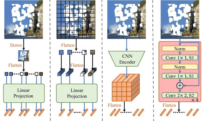
Figure 3: Token representation. (a) Pixel to token. (b) Patch to token. (c) Feature to token. (d) Restrictive Receptive Field (RF) feature to token. Note our token has a small and non-overlapping RF like VIT [11], but uses a stacked (x4) CNN embedding. Each token represents locally isolated patches, leaving the global context relationship to be cleanly modeled in a transformer encoder.

3.1 Content Inference Network: TFill-Coarse

The proposed TFill-Coarse model depends on the self-attention module in a transformer-encoder to equally perceiving global visible context for the completed content generation. Considering the fixed length position embedding and dramatically increased computational cost, we first downsample images with arbitrary sizes to a fixed size, e.g. $256\times 256$. However, it is still not feasible to run a transformer model if we directly flatten image pixels into a 2D sequence with $256\times 256\times 3$ tokens.

To obtain a practicable number of visual tokens, different embedding methods (Fig. 3(a)-(c)) have been used in current visual transformer-based works [11, 6, 62, 12, 8, 16, 19, 47, 60, 46]. These visual tokens’ RF is either as small as a pixel (e.g. iGPT [8]) that loses important context details due to the large-scale downsampling, or is as large as the full image size (e.g. VQGAN [12]) that has firstly been gradually influenced by neighboring pixels in deep CNN layers. While patch embedding [11] achieves impressive performance in many tasks, one-layer linear projection is still not good enough [48]. The detail comparisons are reported in Table 4.3 and Fig. 8.

Restrictive CNN:

In contrast to these methods, our token representation is extracted using a restrictive CNN (Fig. 3(d)) in 4 blocks. In each block, the $1\times 1$ filter and layernorm is applied for non-linear projection, followed by a partial convolution layer [28] that uses a $2$$\times$$2$ filter with stride $2$ to extract visible information. In particular, if half of the regions in a window are masked, we only embed the other $50\%$ comprising visible pixels as our token representation, and establish an initial weight of $0.5$ for the next weighted self-attention layer. To do this, we ensure each token represents only the visible information in a local patch, leaving the long-range dependencies to be explicitly modeled by a transformer, without cross-contamination from implicit correlation due to larger CNN RF.

In fact, some latest works also begin to explore the influence of different token embeddings. Swin [32] used shift windows to get multi-scales embedded features for multi-scales transformer blocks. $\text{ViT}_{c}$ [48] demonstrated an early CNN token embedding is important for visual transformer. However, they do not consider information flowing from visible to masked regions. When a large RF is applied into a deep CNN embedding, the masked holes will be gradually determined by the neighboring visible pixels. In Fig. 4, we empirically show this is precisely the case for prior CNN-based models. Because masked regions originally hold zero values, they will take the neighboring visible pixels as a filled and reasonable value for the next layer. In contrast, as the small patch is directly embedded using local visible information with important weight, the proposed restrictive CNN is better suited for image completion task.

Weighted Self-Attention Layer:

To further encourage the model to bias to the important visible values, we replace the self-attention layer with a weighted self-attention layer, in which a weight is applied to scale the attention scores. The initial weight $w^{(1)}\in(0.02,1.0]$ is obtained by calculating the fraction of visible pixels in a small patch, e.g. $192/(16\times 16)$ means $192$ pixels in the $16\times 16$ patch are visible. It will then be gradually amplified by updating $w^{(i+1)}\leftarrow\sqrt{w^{(i)}}$ after every encoder layer, to reflect visible information flow. This initial ratio for each token is efficiently implemented in our restrictive CNN encoder. The implementation details can be found in Appendix C.1.

CNN-based Decoder:

Following existing works [51, 58, 50], a gradual upsampling decoder is implemented to generate photorealistic images. Instead of generating tokens one-by-one, our model directly predict all tokens in one step, resulting in a much faster testing time than existing transformer-based generation networks [8, 12, 46] (Table 4.3).

Figure 4: An example of information flow in image completion. The position $\textbf{x}_{i}$’s response (flow) is calculated by inferring the Jacobian matrix between it to all pixels in the given masked input. Here, only the highest flows are shown. Our TFill correctly captures long-range visible context flow, even with a large mask splitting two semantically important zones.

Figure 5: Coarse and Refined results. (a) Ground truth. (b) Masked input degraded by free-form masks. (c) Coarse output. (d) Refined output. We can see that the refinement network not only increases image quality to a high resolution ($256^{2}$ vs $512^{2}$), but also encourages the left eyeball to be consistent with the visible right eyeball using our attention-aware layer.

3.2 Appearance Refinement Network: TFill-Refined

Although the proposed TFill-Coarse model correctly infers superiorly reasonable content (shown in Figs. A.1, A.2, and A.3) by equally utilizing the global visible context in every layer, two limitations remain. First, it is not suitable for high-resolution input due to the fixed length position embedding. Second, the realistic completed results may not be fully consistent with the original visible appearances, e.g. the generated left eye having a different shape and color to the visible right eye in Fig. 5 (c).

Attention-Aware Layer (AAL):

To mitigate these issues, a refinement network, trained on high-resolution images, is proposed (Fig. 2 (b)). In particular, to further utilize the visible high-frequency details in global, an Attention-Aware Layer (AAL) is designed to copy long-range information from both encoded and decoded features.

As depicted in Fig. 6, given a decoded feature ${\bf x}_{d}$, we first calculate the attention score of:

$${\bf A}=\phi({\bf x}_{d})^{\intercal}\theta({\bf x}_{d}),$$ (1)

where ${\bf A}_{ij}$ represents the similarity of the $i^{\text{th}}$ feature to the $j^{\text{th}}$ feature, and $\mathbf{\phi}$, $\mathbf{\theta}$ are $1$$\times$$1$ convolution filters.

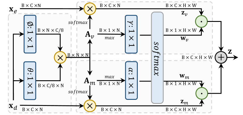
Figure 6: Attention-aware layer. The feature maps are shown as tensors. “$\bigotimes$” denotes matrix multiplication, “$\bigodot$” denotes element-wise multiplication and “$\bigoplus$” is element-wise sum. The blue boxes denote $1\times 1$ convolution filters that are learned.

Interestingly, we discover that using ${\bf A}$ directly in a standard self-attention layer is suboptimal, because the ${\bf x}_{d}$ features for visible regions are generally distinct from those generated for masked regions. Consequently, the attention tends to be insular, with masked regions preferentially attending to masked regions, and vice versa. To avoid this problem, we explicitly handled the attention to visible regions separately from masked regions. So before softmax normalization, ${\bf A}$ is split into two parts: ${\bf A}_{v}$ — similarity to visible regions, and ${\bf A}_{m}$ — similarity to generated masked regions. Next, we get long-range dependencies via:

$$\begin{matrix}{\bf z}_{v}=\texttt{\small softmax}({\bf A}_{v}){\bf x}_{e}&,&{\bf z}_{m}=\texttt{\small softmax}({\bf A}_{m}){\bf x}_{d}\end{matrix}$$ (2)

where ${\bf z}_{v}$ contains features of contextual flow [51] for copying high-frequency details from the encoded high-resolution features ${\bf x}_{e}$ to masked regions, while ${\bf z}_{m}$ has features from the self-attention that is used in SAGAN [55] for high-quality image generation.

Instead of learning fixed weights [58] to combine ${\bf z}_{v}$ and ${\bf z}_{m}$, we learn the weights mapping based on the largest attention score in each position. Specifically, we first obtain the largest attention score of ${\bf A}_{v}$ and ${\bf A}_{m}$, respectively. Then, we use the $1$$\times$$1$ filter $\gamma$ and $\alpha$ to modulate the ratio of the weights. Softmax normalization is applied to ensure ${\bf w}_{v}$$+$${\bf w}_{m}$$=$$1$ in every spatial position:

$$[{\bf w}_{v},{\bf w}_{w}]=\texttt{\small softmax}([\gamma(\texttt{\small max}({\bf A}_{v})),\alpha(\texttt{\small max}({\bf A}_{m})]))$$ (3)

where max is executed on the attention score channel. Finally, an attention-balanced output ${\bf z}$ is obtained by:

$${\bf z}={\bf w}_{v}\cdot{\bf z}_{v}+{\bf w}_{m}\cdot{\bf z}_{m}$$ (4)

where ${\bf w}_{v},{\bf w}_{m}\in\mathbb{R}^{B\times 1\times H\times W}$ hold different values for various positions, dependent on the largest attention scores in the visible and masked regions, respectively.

4 Experiments

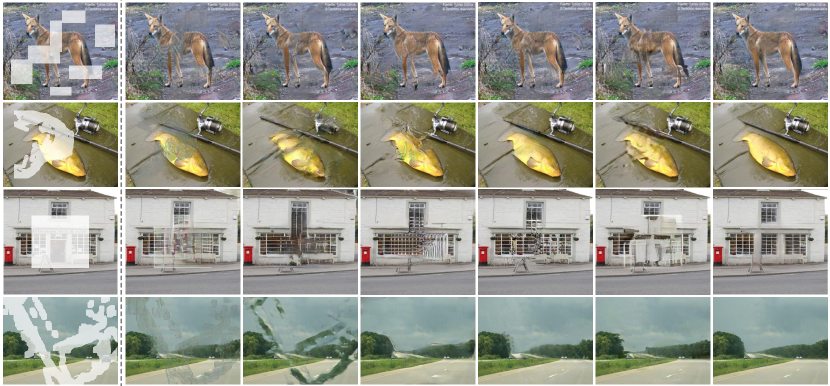
Figure 7: Qualitative comparison on various datasets with free-form masks. Here, we show results for ImageNet [41] (top two examples) and Places2 [61] (bottom two examples). Our model generated more reasonable object and scene structures, with better visual results. Please zoom in to see the details. More comparisons are provided in Figs. A.4, A.5, and A.6.

3.5	PSNR$\uparrow$				SSIM$\uparrow$				LPIPS$\downarrow$				FID$\downarrow$
Mask Ratio	20-30%	30-40%	40-50%		20-30%	30-40%	40-50%		20-30%	30-40%	40-50%		20-30%	30-40%	40-50%
2.5 GL [17]${}_{\text{\scriptsize{SIGGRAPH'2017}}}$	21.33	19.11	17.56		0.7672	0.6823	0.5987		0.1847	0.2535	0.3189		39.22	53.24	68.46
PIC [58]${}_{\text{\scriptsize{CVPR'2019}}}$	24.44	22.32	20.71		0.8520	0.7850	0.7119		0.1183	0.1666	0.2245		21.62	29.59	41.60
DeepFillv2 [52]${}_{\text{\scriptsize{ICCV'2019}}}$	23.58	21.50	19.94		0.8319	0.7712	0.7074		0.1234	0.1639	0.2079		23.18	28.87	35.21
HiFill [50]${}_{\text{\scriptsize{CVPR'2020}}}$	22.54	20.15	18.48		0.7838	0.7057	0.6193		0.1632	0.2258	0.3053		26.89	38.40	56.24
CRFill [53]${}_{\text{\scriptsize{ICCV'2021}}}$	24.38	21.95	20.44		0.8476	0.7983	0.7217		0.1189	0.1597	0.1993		17.58	23.05	29.97
ICT [46]${}_{\text{\scriptsize{ICCV'2021}}}$	24.53	22.84	21.11		0.8599	0.7995	0.7228		0.1045	0.1563	0.1974		17.13	22.39	28.18
Ours TFill	25.10	22.89	21.22		0.8686	0.8063	0.7391		0.0918	0.1328	0.1796		15.28	19.99	25.88
3.5

Table 1: Quantitative comparisons on Places2 [61] with free-form masks [28]. Without bells and whistles, TFill outperformed all existing learning-based models. The results are reported on $256\times 256$ resolution, as earlier works were trained only on this scale.

4.1 Experimental Details

Datasets:

We evaluated the proposed TFill model with arbitrary mask types on various datasets, including CelebA-HQ [33, 22], FFHQ [23], Places2 [61], and ImageNet [41].

Metrics:

Following existing works [35, 46, 59], we mainly reported the traditional patch-level image quality metrics, including peak signal-to-noise ratio (PSNR) and structure similarity index (SSIM), and the latest learned feature-level LPIPS [56] and FID [15] metrics.

Implementation Details:

Our model is trained in two stages: 1) the TFill-Coarse is first trained for $256\times 256$ resolution; and 2) the TFill-Refined is then trained for $512\times 512$ resolution. Unless other noted, TFill indicates the whole model in the paper. Both networks are optimized using the loss $L=L_{pixel}+L_{per}+L_{GAN}$, where $L_{pixel}$ is the $\ell_{1}$ reconstruction loss, $L_{per}$ is the perceptual loss [21], and $L_{GAN}$ is the discriminator loss [13]. More implementation details are provided in Appendix C.

4.2 Main Results

We firstly compared with the following state-of-the-art image completion methods: GL [17]${}_{\text{\scriptsize{SIGGRAPH'2017}}}$, DeepFillv2 [52]${}_{\text{\scriptsize{ICCV'2019}}}$, PIC [58]${}_{\text{\scriptsize{CVPR'2019}}}$, HiFill [50]${}_{\text{\scriptsize{CVPR'2020}}}$, CRFill [53]${}_{\text{\scriptsize{ICCV'2021}}}$, and ICT [46]${}_{\text{\scriptsize{ICCV'2021}}}$ using their publicly released codes and models.

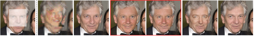
Figure 8: Comparing results under different token representations. All transformers are based on the same transformer backbone  [45]. For VQGAN [12], we report completed (Comp) image and recomposed (Recomp) image. ICT [46] used two-stages networks as the original paper. TFill-Coarse is our model with configure $\mathbb{E}$ in Table 4.2, i.e. TFill w/o the refinement network.

Quantitative Results:

Table 1 shows quantitative evaluation results on Places2 [61], in which the images were degraded by free-form masks provided in the PConv [28] testing set. The mask ratio denotes the range of masking proportion applied to the images. The original mask ratios hold six levels, from 0 to $60\%$, increasing $10\%$ for each level. Here, following ICT [46], we only compare the results on middle-level mask ratios. As can be seen, the proposed TFill model outperformed the CNN-based state-of-the-art models in all mask scales. Spcifically, it achieves averaging relative $18.8\%$ and $13.3\%$ improvements for LPIPS and FID scores, respectively. While the latest ICT [46] also utilized the transformer architecture to capture the global information, they directly downsampled the original image into 32$\times$32, or $48\times 48$ resolution, and then embeded each pixel as a token, resulting in important information is lost during such hard large-scale downsampling.

3.5	Method	CelebA-HQ			FFHQ
		LPIPS$\downarrow$	FID$\downarrow$		LPIPS$\downarrow$	FID$\downarrow$
2     CA [51]${}_{\text{\scriptsize{CVPR'2018}}}$		0.104	9.53		0.127	8.78
PIC [58]${}_{\text{\scriptsize{CVPR'2019}}}$		0.061	6.43		0.068	4.61
MEDFE [29]${}_{\text{\scriptsize{ECCV'2020}}}$		0.067	7.01		-	-
1-7 $\mathbb{A}$	Traditional Conv	0.060	6.29		0.066	4.12
$\mathbb{B}$	+ Attention in G	0.059	6.34		0.064	4.01
$\mathbb{C}$	+ Restrictive Conv	0.056	4.68		0.060	3.87
$\mathbb{D}$	+ Transformer	0.051	4.02		0.057	3.66
$\mathbb{E}$	+ Masked Attention	0.050	3.92		0.057	3.63
$\mathbb{F}$	+ Refine Network	0.048	3.86		0.053	3.50
2

Table 2: Learned Perceptual Image Patch Similarity (LPIPS) and Fréchet Inception Distance (FID) for various completion networks on center masked images. In this paper, we calculate the LPIPS and FID using all images in the corresponding test sets.

Qualitative Results:

The qualitative comparisons are visualized in Figs. 7 and 9. The proposed TFill achieved superior visual results even under challenging conditions. In Fig. 9, we compared with CA [51], PIC [58], and CRFill [53] on Celeba-HQ dataset. Our TFill generates photorealistic high-resolution ($512\times 512$) results, even when significant semantic information is missing.

Fig. 7 shows visual results on natural images that were degraded by random masks. Here, we mainly compared the results for semantic content completion, while visualizing the easily traditional object removal results in Appendix A.3 (Figs. A.7, A.8, and A.9). GL [17], DeepFillv2 [52], and HiFill [50], while good at object removal, failed to infer shapes needed for object completion, e.g. the content for animals. CRFill [53] provided plausible appearance, yet the animals’ shapes are unaligned, e.g. malposed leg and body of the dog. Our TFill inferred the correct shapes for even heavily masked objects in ImageNet, e.g. the fish even with head and tail separated by a large mask. It also outperformed all previous methods on high-resolution masked images in Places2, especially for some large masked regions. More comparisons are presented in Appendix A.2 (Figs. A.4, A.5, A.6). Please zoom in to see the details.

4.3 Ablation Experiments

We ran a number of ablations to analyze the effectiveness of each component in our TFill. Results are shown in Tables 4.2, 4.3, and 4, and Figs. 8 and 9.

TFill Architecture:

We first evaluated components in the redesigned image completion architecture in Table 4.2, which experimentally demonstrates that the new architecture considerably improves the performance. Our baseline configuration ($\mathbb{A}$) used an encoder-decoder structure derived from VQGAN [12], except here attention layers were removed in advance for a pure CNN-baseline. When combined with the powerful discriminator of StyleGANv2 [24], the performance was comparable to previous state-of-the-art CNN-based PIC [58, 59]. We first added the self-attention layer [55], not context mapping from the encoder [51, 58], to the decoder (Generator, G) in ($\mathbb{B}$), but the performance remained similar to baseline ($\mathbb{A}$). Interestingly, when we use the proposed restrictive CNN in ($\mathbb{C}$) to embed information in the local patch, the performance improved substantially, especially for FID (relative $20.2\%$ on CelebA-HQ). This suggests that the input feature representation is significant for the attention layer to equally deliver all messages, as explained in Fig. 4. We then improved this new baseline by adding the transformer encoder ($\mathbb{D}$), which benefits from globally delivered messages at multipe layers. Finally, we introduced masked weights to each attention layer of the transformer ($\mathbb{E}$), improving results further.

Token Representation:

Tables 4.2 and 4.3 report the influence of the token representation. Our TFill achieved much better performance when using the restrictive-CNN. iGPT [8] downsamples the image to a fixed scale, e.g. $32\times 32$, and embeds each pixel to a token. While this may not impact the classification [44], it has a large negative effect on generating high-quality images. Furthermore, the autoregressive form results in the completed image being inconsistent with the bottom-right visible region (Fig. 8 (b)), and each image runs an average of 26.45s on an NVIDIA 1080Ti GPU. ICT [46] improved iGPT by using bidirectional attention and adding a guided upsampling network. While the refined performance can almost match our coarse results, the running time is ruinously expensive (average 152.48s/img) and the content is not aligned well in Figs. 1 and 7. In contrast, VIT [11] embeds each patch to a token. As shown in Table 4.3 and Fig. 8, it can achieve relatively good quantitative and qualitative results. However, some details are perceptually poor, e.g. the strange eyes in Fig. 8. Finally, VQGAN [12] employs a large RF CNN to embed the image. It generates a visually realistic completion (Fig. 8 (d)), but when pasted to the original input (Fig. 8 (e)), there is an obvious gap between generated and visible pixels. When we used large convolutional kernels for large RF (229), the holes will firstly be filled in with neighboring visible pixels, resulting in worse results.

3.5	Method	LPIPS$\downarrow$	FID$\downarrow$	Mem$\downarrow$	Time$\downarrow$
2   IGPT [8]${}_{\text{\scriptsize{ICML'2020}}}$(RF $1$)		0.609	148.42	3.16	26.45
VIT [11]${}_{\text{\scriptsize{ICLR'2021}}}$(RF $16$)		0.062	5.09	1.16	0.167
VQGAN [12]${}_{\text{\scriptsize{CVPR'2021}}}$		0.226	11.92	2.36	4.29
ICT [46]${}_{\text{\scriptsize{ICCV'2021}}}$(RF $1$)		0.061	4.24	3.87	152.48
1-6 $\mathbb{E}$	TFill-Coarse (RF $229$)	0.062	3.92	1.25	0.188
$\mathbb{E}$	TFill-Coarse (RF $16$)	0.057	3.63	1.15	0.180
2

Table 3: The effect of restrictive token representation on FFHQ dataset. “RF” indicates the Receptive Field size. “Mem” denotes the memory (GB) cost during testing and “Time” is the testing time (s) for each center masked image.

3.5	LPIPS$\downarrow$			FID$\downarrow$
Mask Type	center	random		center	random
2 SA [55]${}_{\text{\scriptsize{ICML'19}}}$	0.0584	0.0469		3.62	2.69
CA [51]${}_{\text{\scriptsize{CVPR'2018}}}$	0.0608	0.0443		3.86	2.66
SLTA [58]${}_{\text{\scriptsize{CVPR'2019}}}$	0.0561	0.0452		3.61	2.64
Ours-AAL	0.0533	0.0412		3.50	2.57
2

Table 4: The effect of various attention layers on FFHQ dataset. “center” denotes the center mask, “random” denotes the random mask. These attention layers were implemented within our refinement framework, while using the same content generator.

AAL vs. Others Context Attention Modules:

An evaluation of our proposed AAL is shown in Table 4. For this quantitative experiment we used the same content generator (our TFill-Coarse), but different attention modules in the refinement network. As can be seen, even using the same content, the proposed AAL reduces LPIPS and FID scores by averaging relative $6.0\%$ and $2.8\%$, over the existing works [55, 51, 58]. This is likely due to our AAL selects features based on the largest attention scores, using weights dynamically mapped during inference, instead of depending on fixed weights to copy features as in PIC [58].

The qualitative comparison is visualized in Fig. 9. CA [51], PIC [58], and CRFill [53] used different context attention in image completion. Here, we directly use their publicly models for visualization. As can be seen in the Fig. 9, these state-of-the-art methods cannot handle large holes. While TFill-SA used the good but lower-resolution ($256\times 256$) coarse content from TFill-Coarse, the mouth exhibits artifacts with inconsistent color. Our TFill-AAL (TFill-Refined) shows no such artifacts.

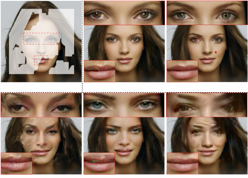
Figure 9: Results with different attention modules in various methods. Our attention-aware layer is able to adaptively select the features from both visible and generated content.

5 Conclusion and Limitation

Through our analyses and experiments, we demonstrate that correctly perceiving and propagating the visible information is significantly important for masked image completion. We experimentally demonstrate the transformer-based architecture has exciting potential for content generation, due to its capacity for effectively modeling soft-connections between distant image content. However, unlike recent vision transformer models that either use shallow projections or large receptive fields for token representation, our restrictive CNN projection provides the necessary separation between explicit global attention modeling and implicit local patch correlation that leads to substantial improvement in results. We also introduced a novel attention-aware layer that adaptively balances the attention for visible and masked regions, further improving the completed image quality.

Limitations:

Although our TFill model outperformed existing state-of-the-art methods on various images that were degraded by random irregular masks, the model is still not able to reason about high-level semantic knowledge. For instance, while our TFill model provided better plausible results in the third row of Fig. 7, it directly redesigned windows based on the visible windows, without understanding the physical world, that a door is necessary for a house. Therefore, a full understanding and imagination of semantic content in an image still needs to be further explored.

Supplementary Material

The supplementary material is organized as follows: in Section A, we first present additional visual results, including results of TFill-Coarse on Face datasets (CelebA-HQ [33, 22], FFHQ [23]), ImageNet [41] and Places2 datasets [56], qualitative comparison to the state-of-the-art models on various datasets, and some examples for free-form editing on high-resolution images. Next, extending the quantitative comparisons of Tables 4.2 in the main paper, Section B presents additional evaluation results under the traditional pixel-level and patch-level image quality metrics. Finally, we discuss more technological details of the proposed TFill model in Section C.

Appendix A Additional Examples

A.1 Additional Results for TFill-Coarse

In Figs. A.1, A.2 and A.3, we show more examples on ImageNet [41], Face datasets (CelebA-HQ [33, 22], FFHQ [23]), and Places2 [56] dataset images that were degraded by large center masks.

Here, all examples shown are chosen from the corresponding testing set. In Fig. A.1, we show examples for object completion, such as the various items and animals on the top half. Fig. A.2 shows visual results of TFill-Coarse on face datasets. In Fig. A.3, we display the completed images for various natural scenes. These examples are good evidence that our TFill model is suitable for both foreground object completion and background scene completion, where it can synthesize semantically consistent content with visually realistic appearance based on the presented visible pixels.

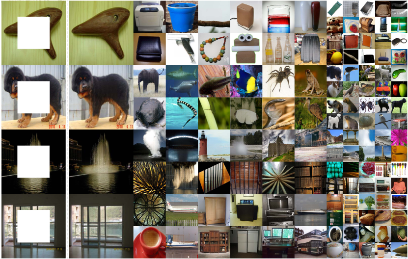
Figure A.1: Example completion results of our method (config $\mathbb{E}$) on ImageNet datasets [41]. All images come from the corresponding testing set that were degraded by center masks. Here, we show results for various categories, such as commodity, animal, plant, natural scene, building, food, furniture and so on. The center masked example inputs are shown on the left. Our model is able to complete both object shape and background scene via a transformer-based architecture to correctly bridge the visible tokens.

Figure A.2: Example completion results of our method (config $\mathbb{E}$) on face datasets. Here, a center mask was used for all input images. One center masked example input is shown top-left. As can be seen, the completed images are on average of high quality. Even for some challenging cases, such as when eyeglasses are center masked, our TFill can correctly repair the face with eyeglasses. Furthermore, it generally works well for varied skin tones, poses, expressions, ages, and illumination.

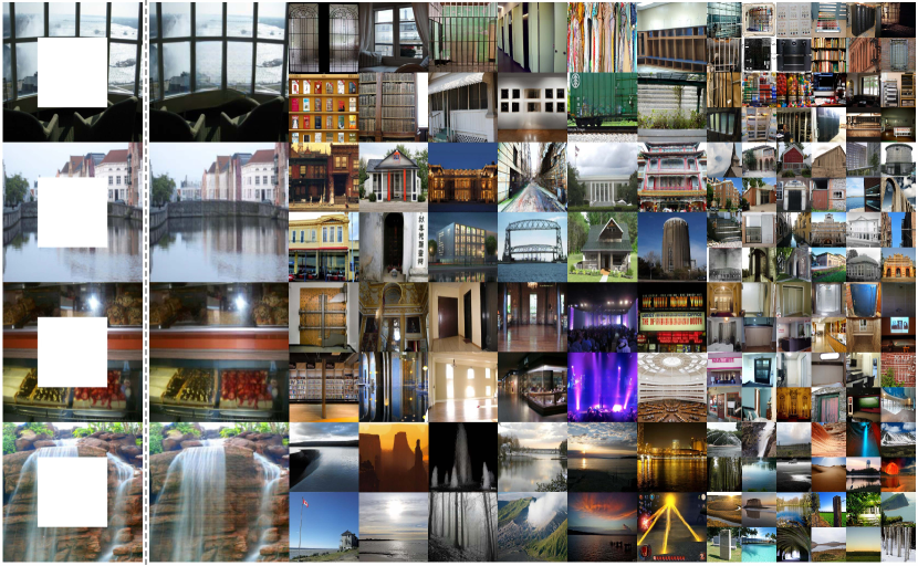
Figure A.3: Example completion results of our method (config $\mathbb{E}$) on Places2 datasets [56]. Here, we show results for varied scene categories. The center masked example inputs are shown on the left. Our model is able to complete both object shape and background scene via a transformer-based architecture to correctly bridge the visible tokens.

A.2 Additional Comparisons

In Figs. A.4, A.5 and A.6, we show additional comparison results on various datasets with free-form masks provided in PConv [28]. This is an extension of Figs. 7 and 9 in the main paper. Here, our results on CelebA-HQ [33, 22] and FFHQ [23] testing set are reported for $512\times 512$ resolution. On the other hand, the results on ImageNet [41] and Places2 [56] are reported for higher resolution images that were resized such that the short side is 512 pixels, with the long side in multiples of $2^{5}=32$, e.g. $640=32\times 20$. The size variability is possible due to our fully convolutional encoder-decoder network structures. The 32-base scale is required because our refinement network downsamples the images 5 times with step 2.

As can be seen from these results, our TFill model filled appropriate semantic content with visually realistic appearance into the various masks. For instance, in the third row of Fig. A.4, even with an extensive mask on an obliquely angled face, it was able to generate high-quality results. It achieved good results even under challenging conditions for various objects (Fig. A.5) and scenes (Fig. A.6).

Figure A.4: Additional results on CelebA-HQ [33, 22] and FFHQ [23] testing set among CA [51], PIC [58], ICT [46] and Ours. Our results are reported for $512^{2}$ resolution. While PIC [58] works well for frontal facing faces, it may generate more uncanny faces with mismatched features at larger angles, e.g. the examples in third and last row. In contrast, our model generated consistent facial features with photorealistic appearance for various faces angles. As ICT [46] does not use context attention in the second stage to copy information from visible pixels, most of eyes on the completed images are inconsistent. Zoom in to see the details.

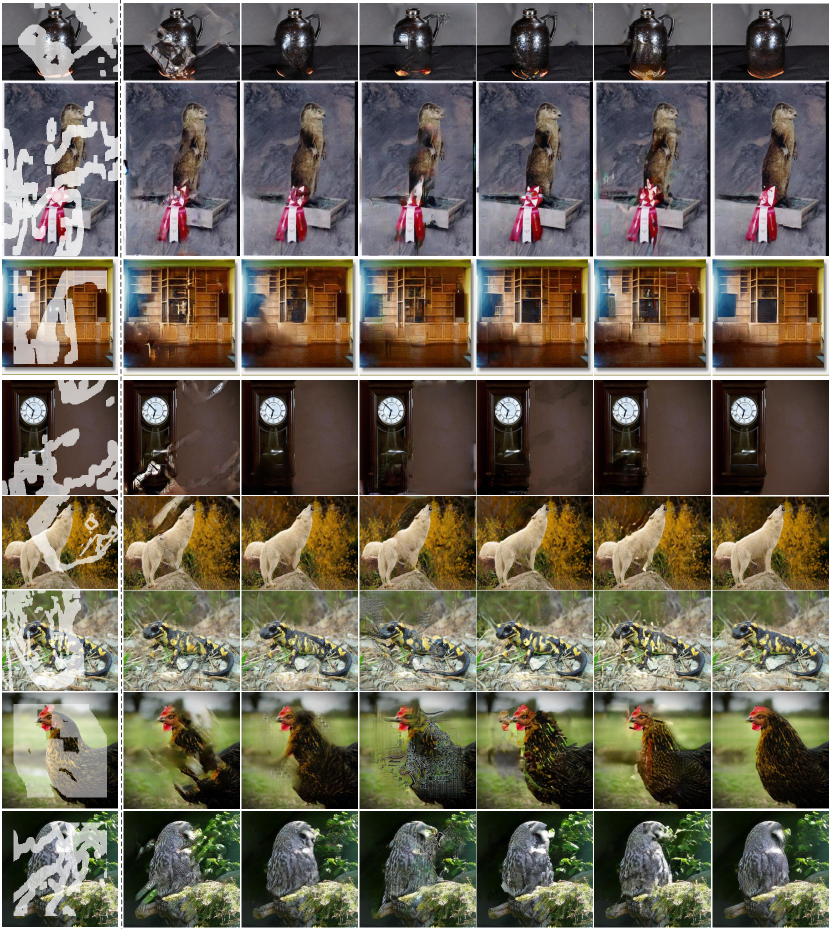
Figure A.5: Additional results on ImageNet [41] testing set among CA [51], PIC [58], HiFill [50], CRFill [53], ICT [46] and Ours. Our results are evaluated in higher resolution, with the short side at $512$ pixels and the long side at multiples of $2^{5}$, e.g. 640. Our TFill model generated better visual results even under very challenging situations, e.g. the heavily masked chicken in the second last row.

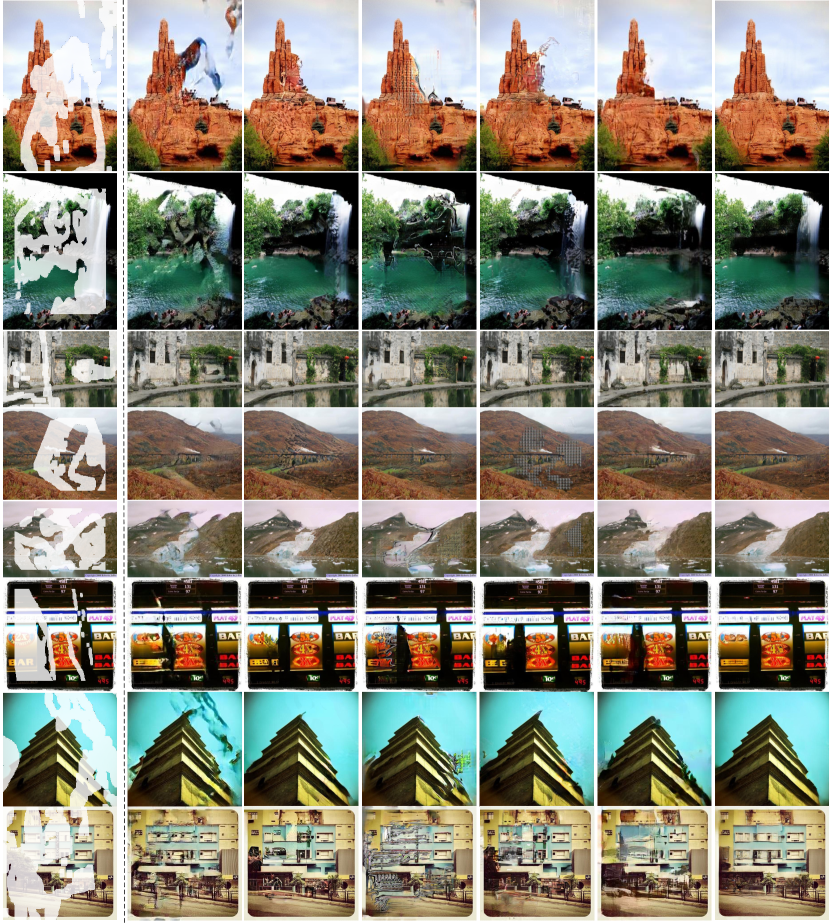
Figure A.6: Additional results on Places2 [56] testing set among CA [51], PIC [58], HiFill [50], CRFill [53], ICT [46] and Ours. Our results are evaluated in higher resolution, with the short side at $512$ pixels and the long side at multiples of $2^{5}$, e.g. 640.

A.3 Free-Form Editing on High-Resolution Images

In Figs. A.7, A.8, A.9 and A.10, we show qualitative results for free-form image masking on various higher resolution datasets.

In Fig. A.7, we show some examples for face editing at $512^{2}$ resolution. For conventional object removal, e.g. watermark removal, our TFill addresses them easily. Furthermore, our TFill can handle more extensive face editing, such as removing substantial facial hair and changing mouth expressions.

In Figs. A.8, A.9 and A.10, we show some examples of editing images of natural / outdoor scenes, with object removal being the main task, as it is the main practice for image inpainting. Here, we enforce the input image size to be multiples of $32$, e.g. $960\times 640$ and provide the high-resolution results on the corresponding image size. As we can see, our TFill-Refined model is able to handle high-resolution images for object removal in traditional image inpainting task.

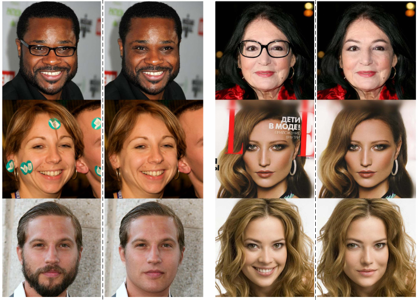
Figure A.7: Additional results on CelebA-HQ [33, 22] and FFHQ [23] testing set for free-form mask editing. All results are reported at $512^{2}$ resolution. Our model works well for traditional object removal, such as removing eyeglasses and watermarks. Furthermore, we provide examples of more substantial modifications, e.g. facial hair removal, and expression modification in the last row.

Figure A.8: Additional free-form editing results on ImageNet [41]. The original image size in ImageNet is $500\times 375$. Here, we resized slightly to $512\times 384$ for image completion. We highlight the generated content, which has consistent textures to those in the visible regions.

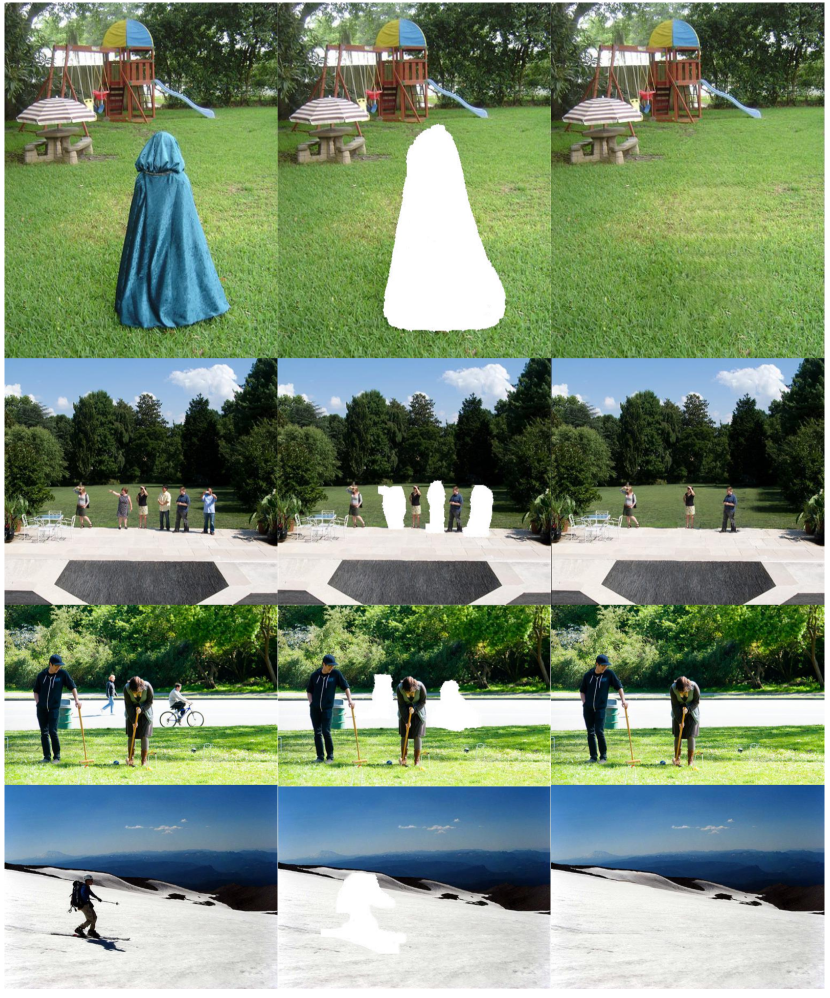
Figure A.9: Additional results on ImageNet [41] testing set for free-form editing. Here, we enforce the input image size to be multiples of $32$, e.g. $960\times 640$ and provide the high-resolution results on the corresponding image size. Zoom in to see the completed details.

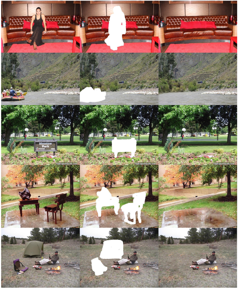
Figure A.10: Additional results on Places2 [56] testing set for free-form editing. Here, we enforce the input image size to be multiples of $32$, e.g. $960\times 640$ and provide the high-resolution results on the corresponding image size. Zoom in to see the completed details.

Appendix B Additional Quantitative Results

We further report quantitative results using traditional pixel-level and patch-level image quality evaluation metrics.

3.5	Method	CelebA-HQ				FFHQ
		$\ell_{1}\text{loss}\downarrow$	SSIM$\uparrow$	PSNR$\uparrow$		$\ell_{1}\text{loss}\downarrow$	SSIM$\uparrow$	PSNR$\uparrow$
2	CA [51]	0.0310	0.8201	23.5667		0.0337	0.8099	22.7745
	PIC [58]	0.0209	0.8668	24.6860		0.0241	0.8547	24.3430
	MEDFE [29]	0.0208	0.8691	24.4733		-	-	-
1-7 $\mathbb{A}$	Traditional Conv	0.0199	0.8693	24.5800		0.0241	0.8559	24.2271
$\mathbb{B}$	+ Attention in G	0.0196	0.8717	24.6512		0.0236	0.8607	24.4384
$\mathbb{C}$	+ Restrictive Conv	0.0191	0.8738	24.8067		0.0220	0.8681	24.9280
$\mathbb{D}$	+ Transformer	0.0189	0.8749	24.9467		0.0197	0.8751	25.1002
$\mathbb{E}$	+ Masked Attention	0.0183	0.8802	25.2510		0.0188	0.8765	25.1204
$\mathbb{F}$	+ Refine Network	0.0180	0.8821	25.4220		0.0184	0.8778	25.2061
2

Table B.1: Quantitative results for traditional pixel-level and patch-level metrics on center masked images.

Table B.1 provides a comparison of our results to state-of-the-art CNN-based models, as well as various alternative configurations for our design, on the center masked face testing set. This is an extension of Table 4.2 in the main paper. All images were normalized to the range [0,1] for quantitative evaluation. While there is no necessity to strongly encourage the completed images to be the same as the original ground-truth images, our TFill model nonetheless achieved better performance on these metrics too, including $\ell_{1}$ loss, structure similarity index (SSIM) and peak signal-to-noise ration (PSNR), suggesting that our TFill model is more capable of generating closer content to the original unmasked images.

Appendix C Experiment Details

Here we first present the novel layers and loss functions used to train our model, followed by the training details.

C.1 Multihead Weighted Self-Attention

Our transformer encoder is built on the standard qkv self-attention (SA) [45] with a learned position embedding in each layer. Given an input sequence $\textbf{z}\in\mathbb{R}^{N\times C}$, we first calculate the pairwise similarity A between each two elements as follows:

$$[\textbf{q},\textbf{k},\textbf{v}] =\textbf{W}_{qkv}\textbf{z}$$ (C.1)

A $$=\texttt{softmax}(\textbf{q}\textbf{k}^{\top}/\sqrt{C_{h}})$$ (C.2)

where $\textbf{W}_{qkv}\in\mathbb{R}^{C\times 3C_{h}}$ is the learned parameter to refine the features z for the query q, the key k and the value v. $\textbf{A}\in\mathbb{R}^{N\times N}$ is the dot similarity of N tokens, which is scaled by the square root of feature dimension $C_{h}$. Then, we compute a weighted sum over all values v via:

$$\text{SA}(\textbf{z})=\textbf{A}\textbf{v}$$ (C.3)

where the value $z$ in the sequence is connected through their learned similarity $A$, rather than purely depending on a fixed learned weight $w$.

The multihead self-attention (MSA) is an extention of SA, in which $H$ heads are run in parallel to get multiple attention scores and the corresponding projected results. Then we get the following function:

$$\text{MSA}(\textbf{z})=[\text{SA}_{1}(\textbf{z});\text{SA}_{2}(\textbf{z});\dots;\text{SA}_{h}(\textbf{z})]$$ (C.4)

To encourage the model to bias to the important visible values, we further modify the MSA with a masked self-attention layer, in which a masked weight is applied to scale the attention score A. Given a feature x and the corresponding mask m (1 denotes visible pixel and 0 is masked pixel). The original partial convolution operation is operated as:

$$x^{\prime} =\begin{cases}\textbf{W}_{p}(\textbf{x}_{p}\bigodot\textbf{m}_{p})\frac{1}{\sum(\textbf{m}_{p})}+b,&\mbox{if}\sum(\textbf{m}_{p})>0\\ 0,&\mbox{otherwise}\end{cases}$$ (C.5)

$$m^{\prime} =\begin{cases}1,&\mbox{if}\sum(\textbf{m}_{p})>0\\ 0,&\mbox{otherwise}\end{cases}$$ (C.6)

where $\textbf{W}_{p}$ contain the convolution filter weights, $b$ is the corresponding bias, while $\textbf{x}_{p}$ and $\textbf{m}_{p}$ are the feature values and mask values in the current convolution window (e.g. $2\times 2$ in our restrictive CNN), respectively. Here, we replace the $m^{\prime}$ as a float value:

$$m^{\prime}=\frac{\sum(\textbf{m}_{p})}{S}$$ (C.7)

where $S$ is the size of each convolution filter, $2\times 2$ used in our restrictive CNN. To do this, each token only extracts the visible information. What’s more, the final $m$ for each token denotes the percentage of valid values in each token under a small RF. Then, for each sequence $\textbf{z}\in\mathbb{R}^{N\times C}$, we obtain a corresponding masked weight $\textbf{m}\in\mathbb{R}^{N\times 1}$ by flattening the updated mask. Finally, we update the original attention score by multiplying with the repeated masked weight $\textbf{m}\in\mathbb{R}^{N\times 1}$:

$$\textbf{A}_{m}=\textbf{A}\bigodot\textbf{m}_{r}$$ (C.8)

where $\textbf{m}_{r}\in\mathbb{R}^{N\times N}$ is the extension of masked weight $\textbf{m}\in\mathbb{R}^{N\times 1}$ in the final dimension.

C.2 Loss Functions

Our work focuses on exploiting the token representation in the visual transformer architecture. We do not modify the discriminator architecture or design the loss function in any way. Both TFill-Coarse and TFill-Refined is trained with loss $L=L_{pixel}+L_{per}+L_{GAN}$. In particular, each loss is given as:

$$L_{pixel} =||\textbf{I}_{gt}-\textbf{I}_{g}||_{1}$$ (C.9)

$$L_{per} =||\Phi_{n}(\textbf{I}_{gt})-\Phi_{n}(\textbf{I}_{g})||_{1}$$ (C.10)

$$L_{GAN} =log(1+\exp(-D(\textbf{I}_{g})))$$ (C.11)

where $\textbf{I}_{g}$ and $\textbf{I}_{gt}$ is the generated image and original ground truth image, respectively. $\Phi_{n}$ is the activation map of the $n$th selected layer in VGG. $D$ is the discriminator and here we show only the generator loss for the generative adversarial traning.

C.3 Training Details

Our model was trained on two NVIDIA A100 GPUs in two stages: 1) the content inference network was first trained with $256^{2}$ resolution with batch size of 96; 2) the visual appearance network was then trained with $512^{2}$ resolution with batch size of 24. Both networks were optimized using the loss $L=L_{pixel}+L_{per}+L_{GAN}$. The design of the encoder-decoder backbone follows the architecture presented in [12]. For the discriminator, we used the architecture of StyleGANv2 [24].

References

- [1] Coloma Ballester, Marcelo Bertalmio, Vicent Caselles, Guillermo Sapiro, and Joan Verdera. Filling-in by joint interpolation of vector fields and gray levels. IEEE transactions on image processing, 10(8):1200–1211, 2001.
- [2] Connelly Barnes, Eli Shechtman, Adam Finkelstein, and Dan B Goldman. Patchmatch: A randomized correspondence algorithm for structural image editing. ACM Transactions on Graphics (ToG), 28:24, 2009.
- [3] Marcelo Bertalmio, Guillermo Sapiro, Vincent Caselles, and Coloma Ballester. Image inpainting. In Proceedings of the 27th annual conference on Computer graphics and interactive techniques, pages 417–424. ACM Press/Addison-Wesley Publishing Co., 2000.
- [4] Marcelo Bertalmio, Luminita Vese, Guillermo Sapiro, and Stanley Osher. Simultaneous structure and texture image inpainting. IEEE transactions on image processing, 12(8):882–889, 2003.
- [5] Chenjie Cao and Yanwei Fu. Learning a sketch tensor space for image inpainting of man-made scenes. In Proceedings of the IEEE/CVF International Conference on Computer Vision (ICCV), pages 14509–14518, October 2021.
- [6] Nicolas Carion, Francisco Massa, Gabriel Synnaeve, Nicolas Usunier, Alexander Kirillov, and Sergey Zagoruyko. End-to-end object detection with transformers. In European Conference on Computer Vision, pages 213–229. Springer, 2020.
- [7] Hanting Chen, Yunhe Wang, Tianyu Guo, Chang Xu, Yiping Deng, Zhenhua Liu, Siwei Ma, Chunjing Xu, Chao Xu, and Wen Gao. Pre-trained image processing transformer. In Proceedings of the IEEE/CVF Conference on Computer Vision and Pattern Recognition, pages 12299–12310, 2021.
- [8] Mark Chen, Alec Radford, Rewon Child, Jeffrey Wu, Heewoo Jun, David Luan, and Ilya Sutskever. Generative pretraining from pixels. In International Conference on Machine Learning, pages 1691–1703. PMLR, 2020.
- [9] Antonio Criminisi, Patrick Pérez, and Kentaro Toyama. Region filling and object removal by exemplar-based image inpainting. IEEE Transactions on image processing, 13(9):1200–1212, 2004.
- [10] Jacob Devlin, Ming-Wei Chang, Kenton Lee, and Kristina Toutanova. Bert: Pre-training of deep bidirectional transformers for language understanding. arXiv preprint arXiv:1810.04805, 2018.
- [11] Alexey Dosovitskiy, Lucas Beyer, Alexander Kolesnikov, Dirk Weissenborn, Xiaohua Zhai, Thomas Unterthiner, Mostafa Dehghani, Matthias Minderer, Georg Heigold, Sylvain Gelly, et al. An image is worth 16x16 words: Transformers for image recognition at scale. In International Conference on Learning Representations, 2021.
- [12] Patrick Esser, Robin Rombach, and Bjorn Ommer. Taming transformers for high-resolution image synthesis. In Proceedings of the IEEE/CVF Conference on Computer Vision and Pattern Recognition, pages 12873–12883, 2021.
- [13] Ian Goodfellow, Jean Pouget-Abadie, Mehdi Mirza, Bing Xu, David Warde-Farley, Sherjil Ozair, Aaron Courville, and Yoshua Bengio. Generative adversarial nets. In Advances in neural information processing systems, pages 2672–2680, 2014.
- [14] Kaiming He, Xinlei Chen, Saining Xie, Yanghao Li, Piotr Dollár, and Ross Girshick. Masked autoencoders are scalable vision learners. arXiv preprint arXiv:2111.06377, 2021.
- [15] Martin Heusel, Hubert Ramsauer, Thomas Unterthiner, Bernhard Nessler, and Sepp Hochreiter. Gans trained by a two time-scale update rule converge to a local nash equilibrium. In Advances in neural information processing systems, pages 6626–6637, 2017.
- [16] Drew A Hudson and C. Lawrence Zitnick. Generative adversarial transformers. arXiv preprint, 2021.
- [17] Satoshi Iizuka, Edgar Simo-Serra, and Hiroshi Ishikawa. Globally and locally consistent image completion. ACM Transactions on Graphics (ToG), 36(4):1–14, 2017.
- [18] Jiaya Jia and Chi-Keung Tang. Inference of segmented color and texture description by tensor voting. IEEE Transactions on Pattern Analysis and Machine Intelligence, 26(6):771–786, 2004.
- [19] Yifan Jiang, Shiyu Chang, and Zhangyang Wang. Transgan: Two transformers can make one strong gan. arXiv preprint arXiv:2102.07074, 2021.
- [20] Youngjoo Jo and Jongyoul Park. Sc-fegan: face editing generative adversarial network with user’s sketch and color. In Proceedings of the IEEE/CVF International Conference on Computer Vision, pages 1745–1753, 2019.
- [21] Justin Johnson, Alexandre Alahi, and Li Fei-Fei. Perceptual losses for real-time style transfer and super-resolution. In European conference on computer vision, pages 694–711. Springer, 2016.
- [22] Tero Karras, Timo Aila, Samuli Laine, and Jaakko Lehtinen. Progressive growing of gans for improved quality, stability, and variation. In International Conference on Learning Representations, 2018.
- [23] Tero Karras, Samuli Laine, and Timo Aila. A style-based generator architecture for generative adversarial networks. In Proceedings of the IEEE/CVF Conference on Computer Vision and Pattern Recognition, pages 4401–4410, 2019.
- [24] Tero Karras, Samuli Laine, Miika Aittala, Janne Hellsten, Jaakko Lehtinen, and Timo Aila. Analyzing and improving the image quality of stylegan. In Proceedings of the IEEE/CVF Conference on Computer Vision and Pattern Recognition, pages 8110–8119, 2020.
- [25] Diederik P. Kingma and Max Welling. Auto-encoding variational bayes. In 2nd International Conference on Learning Representations, ICLR 2014, Banff, AB, Canada, April 14-16, 2014, Conference Track Proceedings, 2014.
- [26] Anat Levin, Assaf Zomet, and Yair Weiss. Learning how to inpaint from global image statistics. In ICCV, volume 1, pages 305–312, 2003.
- [27] Liang Liao, Jing Xiao, Zheng Wang, Chia-Wen Lin, and Shin’ichi Satoh. Image inpainting guided by coherence priors of semantics and textures. In Proceedings of the IEEE/CVF Conference on Computer Vision and Pattern Recognition, pages 6539–6548, 2021.
- [28] Guilin Liu, Fitsum A. Reda, Kevin J. Shih, Ting-Chun Wang, Andrew Tao, and Bryan Catanzaro. Image inpainting for irregular holes using partial convolutions. In Proceedings of the European Conference on Computer Vision (ECCV), September 2018.
- [29] Hongyu Liu, Bin Jiang, Yibing Song, Wei Huang, and Chao Yang. Rethinking image inpainting via a mutual encoder-decoder with feature equalizations. In Proceedings of the European Conference on Computer Vision, 2020.
- [30] Hongyu Liu, Ziyu Wan, Wei Huang, Yibing Song, Xintong Han, and Jing Liao. Pd-gan: Probabilistic diverse gan for image inpainting. In Proceedings of the IEEE/CVF Conference on Computer Vision and Pattern Recognition, pages 9371–9381, 2021.
- [31] Rui Liu, Hanming Deng, Yangyi Huang, Xiaoyu Shi, Lewei Lu, Wenxiu Sun, Xiaogang Wang, Jifeng Dai, and Hongsheng Li. Fuseformer: Fusing fine-grained information in transformers for video inpainting. In International Conference on Computer Vision (ICCV), 2021.
- [32] Ze Liu, Yutong Lin, Yue Cao, Han Hu, Yixuan Wei, Zheng Zhang, Stephen Lin, and Baining Guo. Swin transformer: Hierarchical vision transformer using shifted windows. International Conference on Computer Vision (ICCV), 2021.
- [33] Ziwei Liu, Ping Luo, Xiaogang Wang, and Xiaoou Tang. Deep learning face attributes in the wild. In Proceedings of International Conference on Computer Vision (ICCV), December 2015.
- [34] Mehdi Mirza and Simon Osindero. Conditional generative adversarial nets. arXiv preprint arXiv:1411.1784, 2014.
- [35] Kamyar Nazeri, Eric Ng, Tony Joseph, Faisal Qureshi, and Mehran Ebrahimi. Edgeconnect: Structure guided image inpainting using edge prediction. In The IEEE International Conference on Computer Vision (ICCV) Workshops, Oct 2019.
- [36] Deepak Pathak, Philipp Krahenbuhl, Jeff Donahue, Trevor Darrell, and Alexei A Efros. Context encoders: Feature learning by inpainting. In Proceedings of the IEEE Conference on Computer Vision and Pattern Recognition, pages 2536–2544, 2016.
- [37] Jialun Peng, Dong Liu, Songcen Xu, and Houqiang Li. Generating diverse structure for image inpainting with hierarchical vq-vae. In Proceedings of the IEEE/CVF Conference on Computer Vision and Pattern Recognition (CVPR), pages 10775–10784, 2021.
- [38] Tiziano Portenier, Qiyang Hu, Attila Szabo, Siavash Arjomand Bigdeli, Paolo Favaro, and Matthias Zwicker. Faceshop: Deep sketch-based face image editing. ACM Transactions on Graphics (TOG), 37(4):99, 2018.
- [39] Alec Radford, Karthik Narasimhan, Tim Salimans, and Ilya Sutskever. Improving language understanding by generative pre-training. Technical report, OpenAI, 2018.
- [40] Alec Radford, Jeffrey Wu, Rewon Child, David Luan, Dario Amodei, and Ilya Sutskever. Language models are unsupervised multitask learners. OpenAI blog, 1(8):9, 2019.
- [41] Olga Russakovsky, Jia Deng, Hao Su, Jonathan Krause, Sanjeev Satheesh, Sean Ma, Zhiheng Huang, Andrej Karpathy, Aditya Khosla, Michael Bernstein, et al. Imagenet large scale visual recognition challenge. International Journal of Computer Vision, 115(3):211–252, 2015.
- [42] Yuhang Song, Chao Yang, Zhe Lin, Xiaofeng Liu, Qin Huang, Hao Li, and C-C Jay Kuo. Contextual-based image inpainting: Infer, match, and translate. In Proceedings of the European Conference on Computer Vision (ECCV), pages 3–19, 2018.
- [43] Yuhang Song, Chao Yang, Yeji Shen, Peng Wang, Qin Huang, and C-C Jay Kuo. Spg-net: Segmentation prediction and guidance network for image inpainting. arXiv preprint arXiv:1805.03356, 2018.
- [44] Antonio Torralba, Rob Fergus, and William T Freeman. 80 million tiny images: A large data set for nonparametric object and scene recognition. IEEE transactions on pattern analysis and machine intelligence, 30(11):1958–1970, 2008.
- [45] Ashish Vaswani, Noam Shazeer, Niki Parmar, Jakob Uszkoreit, Llion Jones, Aidan N Gomez, Ł ukasz Kaiser, and Illia Polosukhin. Attention is all you need. In I. Guyon, U. V. Luxburg, S. Bengio, H. Wallach, R. Fergus, S. Vishwanathan, and R. Garnett, editors, Advances in Neural Information Processing Systems, volume 30. Curran Associates, Inc., 2017.
- [46] Ziyu Wan, Jingbo Zhang, Dongdong Chen, and Jing Liao. High-fidelity pluralistic image completion with transformers. In Proceedings of the IEEE/CVF International Conference on Computer Vision (ICCV), pages 4692–4701, October 2021.
- [47] Bichen Wu, Chenfeng Xu, Xiaoliang Dai, Alvin Wan, Peizhao Zhang, Masayoshi Tomizuka, Kurt Keutzer, and Peter Vajda. Visual transformers: Token-based image representation and processing for computer vision. arXiv preprint arXiv:2006.03677, 2020.
- [48] Tete Xiao, Mannat Singh, Eric Mintun, Trevor Darrell, Piotr Dollár, and Ross Girshick. Early convolutions help transformers see better. arXiv preprint arXiv:2106.14881, 2021.
- [49] Zhaoyi Yan, Xiaoming Li, Mu Li, Wangmeng Zuo, and Shiguang Shan. Shift-net: Image inpainting via deep feature rearrangement. In Proceedings of the European conference on computer vision (ECCV), pages 1–17, 2018.
- [50] Zili Yi, Qiang Tang, Shekoofeh Azizi, Daesik Jang, and Zhan Xu. Contextual residual aggregation for ultra high-resolution image inpainting. In Proceedings of the IEEE/CVF Conference on Computer Vision and Pattern Recognition, pages 7508–7517, 2020.
- [51] Jiahui Yu, Zhe Lin, Jimei Yang, Xiaohui Shen, Xin Lu, and Thomas S Huang. Generative image inpainting with contextual attention. In Proceedings of the IEEE Conference on Computer Vision and Pattern Recognition, pages 5505–5514, 2018.
- [52] Jiahui Yu, Zhe Lin, Jimei Yang, Xiaohui Shen, Xin Lu, and Thomas S Huang. Free-form image inpainting with gated convolution. In Proceedings of the IEEE/CVF International Conference on Computer Vision, pages 4471–4480, 2019.
- [53] Yu Zeng, Zhe Lin, Huchuan Lu, and Vishal M. Patel. Cr-fill: Generative image inpainting with auxiliary contextual reconstruction. In Proceedings of the IEEE International Conference on Computer Vision, 2021.
- [54] Yu Zeng, Zhe Lin, Jimei Yang, Jianming Zhang, Eli Shechtman, and Huchuan Lu. High-resolution image inpainting with iterative confidence feedback and guided upsampling. In European Conference on Computer Vision, pages 1–17. Springer, 2020.
- [55] Han Zhang, Ian Goodfellow, Dimitris Metaxas, and Augustus Odena. Self-attention generative adversarial networks. In International conference on machine learning, pages 7354–7363. PMLR, 2019.
- [56] Richard Zhang, Phillip Isola, Alexei A Efros, Eli Shechtman, and Oliver Wang. The unreasonable effectiveness of deep features as a perceptual metric. In CVPR, 2018.
- [57] Lei Zhao, Qihang Mo, Sihuan Lin, Zhizhong Wang, Zhiwen Zuo, Haibo Chen, Wei Xing, and Dongming Lu. Uctgan: Diverse image inpainting based on unsupervised cross-space translation. In Proceedings of the IEEE/CVF Conference on Computer Vision and Pattern Recognition, pages 5741–5750, 2020.
- [58] Chuanxia Zheng, Tat-Jen Cham, and Jianfei Cai. Pluralistic image completion. In Proceedings of the IEEE/CVF Conference on Computer Vision and Pattern Recognition (CVPR), June 2019.
- [59] Chuanxia Zheng, Tat-Jen Cham, and Jianfei Cai. Pluralistic free-form image completion. International Journal of Computer Vision, pages 1–20, 2021.
- [60] Sixiao Zheng, Jiachen Lu, Hengshuang Zhao, Xiatian Zhu, Zekun Luo, Yabiao Wang, Yanwei Fu, Jianfeng Feng, Tao Xiang, Philip HS Torr, et al. Rethinking semantic segmentation from a sequence-to-sequence perspective with transformers. In Proceedings of the IEEE/CVF Conference on Computer Vision and Pattern Recognition, pages 6881–6890, 2021.
- [61] Bolei Zhou, Agata Lapedriza, Aditya Khosla, Aude Oliva, and Antonio Torralba. Places: A 10 million image database for scene recognition. IEEE transactions on pattern analysis and machine intelligence, 40(6):1452–1464, 2018.
- [62] Xizhou Zhu, Weijie Su, Lewei Lu, Bin Li, Xiaogang Wang, and Jifeng Dai. Deformable detr: Deformable transformers for end-to-end object detection. In International Conference on Learning Representations, 2021.