Plasmon modes of coupled quantum Hall edge channels in the presence of disorder-induced tunneling

Abstract

Coupled quantum Hall edge channels show intriguing non-trivial modes, for example, charge and neutral modes at Landau level filling factors 2 and 2/3. We propose an appropriate and effective model with Coulomb interaction and disorder-induced tunneling characterized by coupling capacitances and tunneling conductances, respectively. This model explains how the transport eigenmodes, within the interaction- and disorder-dominated regimes, change with the coupling capacitance, tunneling conductance, and measurement frequency. We propose frequency- and time-domain transport experiments, from which eigenmodes can be determined using this model.

I Introduction

Integer and fractional quantum Hall systems provide unique opportunities for studying many-body effects in two-dimensional topological insulators, where chiral one-dimensional edge channels dominate the transport characteristics BookEzawa ; BookWen . Particularly, when multiple edge channels are mutually coupled, the system can exhibit fractionalization into non-trivial excitations BookWen ; BookGiamarchi . The phenomena can be understood by considering the transport eigenmodes of the channels. For example, copropagating integer channels along the edge of the quantum Hall state at the Landau level filling factor $\nu=2$ can be understood with the spin and charge (dipolar) modes, where Tomonaga-Luttinger physics show up Bocquillon-NatCom2013 ; Inoue-PRL2014 ; Hashisaka-NatPhys2017 . For another important example of counterpropagating integer and fractional channels at $\nu=2/3$, similar charge and neutral modes can be studied with the edge reconstruction in the hole-conjugate fractional state Bid-PRL2009 ; Sabo-NatPhys17 ; Lafont-Science2019 .

These examples have been studied by utilizing mesoscopic functional devices such as quantum point contacts and quantum dots to reveal non-equilibrium states and their dynamics Ji-Nature03 ; Kamata-PRB10 ; Altimiras-NatPhys10 ; Kamata-NatNano2014 ; Itoh-PRL18 . However, the above two cases have been studied separately as the underlying mechanisms are largely different. While the spin and charge modes at $\nu=2$ are formed by the Coulomb interaction between the channels Berg-PRL2009 , the charge and neutral modes at $\nu=2/3$ arise from disorder-induced tunneling between the channels KaneFisher-PRB1995 ; KaneFisherPolchinski-PRL1994 . As a result, the characteristics of the $\nu$ = 2 and $\nu$ = 2/3 modes are also different. The spin and charge modes at $\nu=2$ cannot be detected at equilibrium with conventional conductance measurements, but can be identified by using methods such as high-frequency transport, shot noise detection, energy-resolved measurements Bocquillon-NatCom2013 ; Inoue-PRL2014 ; Hashisaka-NatPhys2017 . On the other hand, the charge and neutral modes at $\nu=2/3$ can be discussed with the linear conductance that changes with the channel length Grivnin-PRL2014 ; CJLin-PRB2019 . In addition to these individually successful investigations of each system, it would be advantageous to coherently understand the two cases, because actual devices may involve both interaction and tunneling. Indeed, a recent high-frequency experiment supports the emergence of pure neutral and charge modes in the $\nu=2$ system in the presence of tunneling CJLin . There may also be some cases where disorder-induced scattering is suppressed in the $\nu=2/3$ case. Therefore, it is beneficial to consider both interaction and tunneling in the theoretical model, as well as in the experimental analysis.

In this paper, we provide a plasmon scattering model for two parallel edge channels in the presence of arbitrary interaction and tunneling occurring between them, particularly focusing on the eigenmodes of the $\nu=2$ and $\nu=2/3$ cases. Using this model, the manner in which transport eigenmodes change from the uncoupled regime to the interaction-dominated regime and the disorder-dominated regime can be understood systematically by tuning the parameters. The transport eigenmodes can be investigated experimentally by measuring the scattering matrix elements of plasmons for a finite length of the coupled edge channels. The model can be extended to multiple (more than two) channels, as well as other 2D topological insulators where the coupling of multiple channels plays an essential role.

II Plasmon model

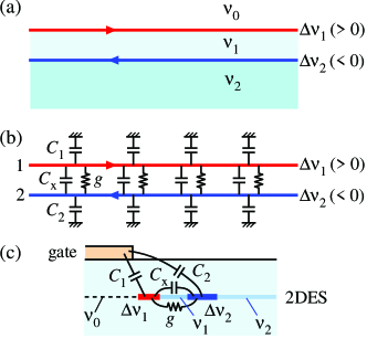
Figure 1: (a) Schematic of the coupled edge channels with $\Delta\nu_{1}=\nu_{1}-\nu_{0}$ and $\Delta\nu_{2}=\nu_{2}-\nu_{1}$ formed along the boundaries of quantum Hall states at $\nu_{0}$, $\nu_{1}$, and $\nu_{2}$. Righ-moving channel with $\Delta\nu_{1}>0$ and left-moving channel with $\Delta\nu_{1}<0$ are illustrated. (b) Plasmon model with distributed capacitances, $C_{1}$, $C_{2}$, and $C_{\mathrm{x}}$, and distributed tunneling conductance $g$. (c) Realistic geometry of the coupled edge channels formed along the perimeter of the gate. Two channels with $\Delta\nu_{1}$ and $\Delta\nu_{2}$ are formed along boundaries of insulation regions with $\nu_{0}$, $\nu_{1}$, and $\nu_{2}$.

We apply a plasmon scattering approach developed with one-dimensional systems BookGiamarchi ; Safi-PRB1995 ; SafiEurPhys ; Hashisaka-PRB2012 ; Protopopov-AnnPhys2017 .We consider two chiral edge channels, $c=\left\{1,2\right\}$, along the boundaries of the quantum Hall (insulating) regions with Landau level filling factors, $\nu_{0}$, $\nu_{1}$, and $\nu_{2}$, as shown in Fig. 1(a). The Hall conductance $\sigma_{c}=\sigma_{q}\Delta\nu_{c}$ of channel $c$ is given by the difference of the filling factor $\Delta\nu_{c}=\nu_{c}-\nu_{c-1}$ in the neighboring regions and quantized conductance $\sigma_{q}=e^{2}/h$. The sign of $\Delta\nu_{c}$ determines the chirality; positive for right movers and negative for left movers.

For example, two copropagating integer channels, $\Delta\nu_{1}=\Delta\nu_{2}=1$, which we shall call the $\nu=2$ case, are formed with $\nu_{0}=0$, $\nu_{1}=1$, and $\nu_{2}=2$ BookEzawa ; Berg-PRL2009 . Two counterpropagating integer/fractional channels, $\Delta\nu_{1}=1$ and $\Delta\nu_{2}=-1/3$, which we shall call the $\nu=2/3$ case, can be studied with $\nu_{0}=0$, $\nu_{1}=1$, and $\nu_{2}=2/3$ MacDonald-PRL1990 ; Wen-PRL1990 . The interactions between the channels, as well as those within each channel, can be described with mutual capacitance $C_{\mathrm{x}}$ and self capacitances $C_{\mathrm{1}}$ and $C_{\mathrm{2}}$ defined for a unit length, as shown in Fig. 1(b) Hashisaka-NatPhys2017 . The self capacitances are practically determined by capacitances to the ground, such as nearby gate electrodes or a potential reference. The disorder-induced tunneling can be described with tunneling conductance $g$ defined for the unit length Nosiglia-PRB2018 .

Such edge channels can be formed in a gated AlGaAs/GaAs heterostructure, as shown in Fig. 1(c). The bulk of the 2DEG on the right side is prepared in a QH state at $\nu_{2}$, and the application of a negative voltage on the surface metal gate depletes the underlying 2DEG on the left side to set $\nu_{0}=0$. A narrow QH state at $\nu_{1}$ is formed for specific choices of $\nu_{2}$ and $\nu_{0}$. Interactions for the system comprising the channels, $\Delta\nu_{1}$ and $\Delta\nu_{2}$, are described with geometric capacitances $C_{\mathrm{1}}$, $C_{\mathrm{2}}$, and $C_{\mathrm{x}}$ as illustrated. Tunneling between the channels is allowed in the presence of impurity potential. Besides, spin-flip mechanisms, such as spin-orbit and hyperfine interactions, may be required for the $\nu=2$ case. We focus on the eigenmode in the presence of both interactions and tunneling.

The charge density $\rho_{c}$ per unit length and electrostatic potential $V_{c}$ of channel $c$ are related by

$$\left(\begin{array}[]{c}\rho_{1}\\ \rho_{2}\end{array}\right)=\left(\begin{array}[]{cc}C_{\mathrm{1}}+C_{\mathrm{x}}&-C_{\mathrm{x}}\\ -C_{\mathrm{x}}&C_{\mathrm{2}}+C_{\mathrm{x}}\end{array}\right)\left(\begin{array}[]{c}V_{1}\\ V_{2}\end{array}\right),$$ (1)

which can be written as $\mathbf{\rho}=\mathbf{CV}$ with corresponding vector notations, $\mathbf{\rho}=\left(\begin{array}[]{c}\rho_{1}\\ \rho_{2}\end{array}\right)$ and $\mathbf{V}=\left(\begin{array}[]{c}V_{1}\\ V_{2}\end{array}\right)$, and the capacitance matrix $\mathbf{C}$. Here, $\mathbf{\rho}$ and $\mathbf{V}$ change with time $t$ and coordinate $x$. The electrochemical potential $\mu_{c}=eV_{c}+\rho_{c}/D_{c}$ is further raised by the second term with the density of states $D_{c}$ Gabelli-PRL2007 ; Hashisaka-RevPhys2018 . By using its matrix form $\mathbf{D}=\left(\begin{array}[]{cc}D_{1}&0\\ 0&D_{2}\end{array}\right)$, the vector form of $\mathbf{\mu}=\left(\begin{array}[]{c}\mu_{1}\\ \mu_{2}\end{array}\right)$ is given by

$$\mathbf{\mu}=\left(e\mathbf{C}^{-1}+\mathbf{D}^{-1}\right)\mathbf{\rho}=e\mathbf{\mathbf{\bar{C}}}^{-1}\mathbf{\rho.}$$ (2)

For convenience, we use effective capacitance matrix $\mathbf{\bar{C}}$ defined as $\mathbf{\bar{C}}^{-1}=\mathbf{C}^{-1}+\mathbf{D}^{-1}/e$. Its matrix elements can be written as

$$\mathbf{\bar{C}=}\left(\begin{array}[]{cc}\bar{C}_{\mathrm{1}}+\bar{C}_{\mathrm{x}}&-\bar{C}_{\mathrm{x}}\\ -\bar{C}_{\mathrm{x}}&\bar{C}_{\mathrm{2}}+\bar{C}_{\mathrm{x}}\end{array}\right),$$ (3)

where $\bar{C}_{\mathrm{1}}$, $\bar{C}_{\mathrm{2}}$, and $\bar{C}_{\mathrm{x}}$ approach $C_{\mathrm{1}}$, $C_{\mathrm{2}}$, and $C_{\mathrm{x}}$, respectively, of Eq. (1) in the limit of large $D_{c}$ ($\gg C_{c}$). For a soft edge potential with large $D_{c}$, such as in AlGaAs/GaAs heterostructures ($\mathbf{C}^{-1}\gg\mathbf{D}^{-1}/e$), $\mathbf{\bar{C}}$ can be approximated to the geometric capacitance matrix $\mathbf{C}$. Nevertheless, we shall use $\mathbf{\bar{C}}$ in the following analysis.

The difference in the electrochemical potentials induces a tunneling current $I_{\mathrm{x}}=g\left(\mu_{2}-\mu_{1}\right)/e$ between the channels. The resulting current $I_{\mathrm{c}}$ on channel $c$ is determined by the charge conservation ($\partial\rho_{1}/\partial t=-\partial I_{1}/\partial x+I_{\mathrm{x}}$, $\partial\rho_{2}/\partial t=-\partial I_{2}/\partial x-I_{\mathrm{x}}$), which can be written as

$$\frac{\partial}{\partial t}\mathbf{\rho=-}\frac{\partial}{\partial x}\mathbf{I-g\mu}/e$$ (4)

with current $\mathbf{I}=\left(\begin{array}[]{c}I_{1}\\ I_{2}\end{array}\right)$ and tunneling conductance $\mathbf{g}=g\left(\begin{array}[]{cc}1&-1\\ -1&1\end{array}\right)$. As the current is related to the electrochemical potential ($\mathbf{I}=\mathbf{\sigma\mu}/e$) with the conductance matrix $\mathbf{\sigma}=\left(\begin{array}[]{cc}\sigma_{1}&0\\ 0&\sigma_{2}\end{array}\right)$, the differential equation can be written in terms of $\mathbf{I}$ as

$$\frac{\partial}{\partial t}\mathbf{I=-\sigma\bar{C}}^{-1}\frac{\partial}{\partial x}\mathbf{I-\sigma\bar{C}}^{-1}\mathbf{g\sigma}^{-1}\mathbf{I.}$$ (5)

This can be used to analyze the dynamics of the current $\mathbf{I}\left(x,t\right)$ as well as the transport eigenmodes of the system. Once $\mathbf{I}$ is determined, one can translate this to the electrochemical potential $\mathbf{\mu}=e\mathbf{\sigma}^{-1}\mathbf{I}$ and the charge density $\mathbf{\rho}=\mathbf{\bar{C}\sigma}^{-1}\mathbf{I}$.

Before solving Eq. (5), we describe the relation to the standard field theory on one-dimensional channels. Generally, the Lagrangian density can be written as

$$L=\frac{\hbar}{4\pi}\sum_{i,j}\left(K_{ij}\partial_{t}\phi_{i}\partial_{x}\phi_{j}+V_{ij}\partial_{x}\phi_{i}\partial_{x}\phi_{j}\right)$$ (6)

for a boson field $\phi_{i}$ on channel $i$, where $\mathbf{K}=\left(K_{ij}\right)$ is an integer-valued symmetric matrix and $\mathbf{V}=\left(V_{ij}\right)$ is a positive definite matrix BookWen ; Wen-PRL1990 . By using the Euler-Lagrange equation $\partial L/\partial\phi_{i}=\partial_{\mu}\left[\partial L/\partial\left(\partial_{\mu}\phi_{i}\right)\right]$ with variable $\mu=\left\{x,t\right\}$, one can derive an equation of motion

$$\sum_{j}K_{ij}\partial_{t}\left(\partial_{x}\phi_{j}\right)=-\sum_{j}V_{ij}\partial_{x}\left(\partial_{x}\phi_{j}\right).$$ (7)

As the charge density $\rho_{i}=-\frac{e}{2\pi}\partial_{x}\phi_{j}$ is related to the field, this can be transformed to

$$\mathbf{K}\frac{\partial}{\partial t}\mathbf{\rho=-V}\frac{\partial}{\partial x}\mathbf{\rho,}$$ (8)

which is equivalent to Eq. (5) until the scattering (second) term. This comparison suggests that the relations $\mathbf{K}=\sigma_{q}\mathbf{\sigma}^{-1}$ and $\mathbf{V}=\sigma_{q}\mathbf{\bar{C}}^{-1}$ exist between the parameters in both models. For instance, velocity parameters $v_{1}$, $v_{2}$, and $v_{12}$, used in Kane et al.’s seminal paper KaneFisherPolchinski-PRL1994 for the $\nu=2/3$ case, can be described with elements of $\mathbf{\bar{C}}$ as

$$v_{1} = \frac{\sigma_{q}\left(\bar{C}_{2}+\bar{C}_{\mathrm{x}}\right)}{\bar{C}_{1}\bar{C}_{2}+\left(\bar{C}_{1}+\bar{C}_{2}\right)\bar{C}_{\mathrm{x}}}$$ (9)

$$v_{2} = \frac{\sigma_{q}\left(\bar{C}_{1}+\bar{C}_{\mathrm{x}}\right)}{\bar{C}_{1}\bar{C}_{2}+\left(\bar{C}_{1}+\bar{C}_{2}\right)\bar{C}_{\mathrm{x}}}$$ (10)

$$v_{12} = \frac{\sigma_{q}\bar{C}_{\mathrm{x}}}{\bar{C}_{1}\bar{C}_{2}+\left(\bar{C}_{1}+\bar{C}_{2}\right)\bar{C}_{\mathrm{x}}}.$$ (11)

With these relations, the parameters in the effective theory can be related to realistic parameters: the capacitances of the channel geometries and the density of states of the channels.

The scattering term, the second term of Eq. (5), has been obtained in the incoherent tunneling regime, where local potential $\mu_{c}\left(x\right)$ is well defined by assuming local equilibrium between successive scattering events Nosiglia-PRB2018 . This has been used to calculate shot noise characteristics and heat transport in fractional quantum Hall systems Spanslatt-PRL2019 ; Park-PRB2019 . Here, we apply Eq. (5) with this scattering term to investigate time-dependent dynamics in the incoherent regime.

III Transport eigenmodes

We shall derive the transport eigenmodes of Eq. (5) at angular frequency $\omega$. As the scattering term is dissipative, the corresponding momentum $k$ generally takes a complex value. By assuming solutions in a form of $\mathbf{I}\left(x,t\right)=\mathbf{\tilde{I}}\exp\left[i\left(kx-\omega t\right)\right]$ with eigenmode $\mathbf{\tilde{I}}$, Eq. (5) is transformed to

$$k\mathbf{\tilde{I}}=\left(\omega\mathbf{\bar{C}\sigma}^{-1}+i\mathbf{g\sigma}^{-1}\right)\mathbf{\tilde{I}}=\mathbf{M\tilde{I},}$$ (12)

from which $\mathbf{\tilde{I}}$ and $k$ can be obtained by diagonalizing $\mathbf{M}=\left(\omega\mathbf{\bar{C}}+i\mathbf{g}\right)\mathbf{\sigma}^{-1}$.

It is convenient to introduce dimensionless parameters

$$\xi = \frac{\omega\bar{C}_{\mathrm{x}}+ig}{\omega\left(\bar{C}_{1}-m\bar{C}_{2}\right)}$$ (13)

$$m = \sigma_{1}/\sigma_{2}$$ (14)

to characterize the modes, where $m=1$ for the $\nu=2$ case and $m=-3$ for the $\nu=2/3$ case. The complex value $\xi$ determines the relative strength of the interaction ($\bar{C}_{\mathrm{x}}$) in the real part and of the tunneling ($g$) in the imaginary part. The two eigenmodes (labeled by I and II) are written as

$$\mathbf{\tilde{I}}_{\mathrm{I}} = \binom{1}{\tilde{I}_{\mathrm{I}}}\text{ with }\tilde{I}_{\mathrm{I}}=\frac{-2\xi}{1+\left(1-m\right)\xi+X_{m}\left(\xi\right)}$$ (15)

$$\mathbf{\tilde{I}}_{\mathrm{II}} = \binom{\tilde{I}_{\mathrm{II}}}{1}\text{ with }\tilde{I}_{\mathrm{II}}=\frac{1+\left(1-m\right)\xi-X_{m}\left(\xi\right)}{-2\xi}$$ (16)

where the $\xi$ dependent function $X_{m}\left(\xi\right)$ is defined as

$$X_{m}\left(\xi\right)=\sqrt{1+2\left(1-m\right)\xi+\left(1+m\right)^{2}\xi^{2}}.$$ (17)

The corresponding $k$ values are obtained as

$$k_{\mathrm{I}} = \frac{\omega}{2\sigma_{1}}\{\bar{C}_{1}\left[1+\left(1+m\right)\xi+X_{m}\left(\xi\right)\right]$$

$$+m\bar{C}_{2}\left[1-\left(1+m\right)\xi-X_{m}\left(\xi\right)\right]\}$$

$$k_{\mathrm{II}} = \frac{\omega}{2\sigma_{1}}\{\bar{C}_{1}\left[1+\left(1+m\right)\xi-X_{m}\left(\xi\right)\right]$$

$$+m\bar{C}_{2}\left[1-\left(1+m\right)\xi+X_{m}\left(\xi\right)\right]\}$$

for mode I and II, respectively.

In this way, the eigenmodes, $\mathbf{\tilde{I}}_{\mathrm{I}}$ and $\mathbf{\tilde{I}}_{\mathrm{II}}$, can be written with a single complex parameter $\xi=\xi^{\prime}+i\xi^{\prime\prime}$ with the real part $\xi^{\prime}$ and the imaginary part $\xi^{\prime\prime}$. Mode I and II approach the isolated channels 1 and 2, respectively, in the limit of $\xi\longrightarrow 0$. In the limit of either $\xi\longrightarrow\infty$ or $\xi\longrightarrow i\infty$, the eigenmodes approach the pure neutral mode $\binom{1}{-1}$ with vanishing total current and the pure charge mode $\binom{m}{1}$ with equal electrochemical potential $\mathbf{\mu}\propto\binom{1}{1}$.

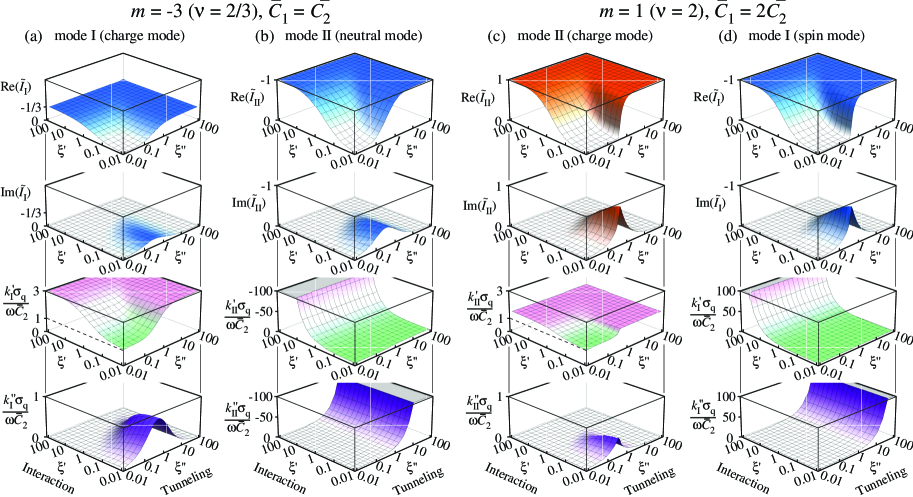
Figure 2: (a and b) Plasmon eigenmodes for the $\nu=2/3$ case ($m=-3$) with $\bar{C}_{1}=\bar{C}_{2}$. Mode I in (a) and mode II in (b) show the (quasi-) charge mode and the (quasi-) neutral mode, respectively. (c and d) Plasmon eigenmodes for the $\nu=2$ case ($m=1$) with $\bar{C}_{1}=2\bar{C}_{2}$. Mode II in (c) and mode I in (d) show the (quasi-) charge mode and the (quasi-) spin mode, respectively. Each system can be characterized by dimensionless parameters, $\xi^{\prime}$ for the interaction and $\xi^{\prime\prime}$ for the tunneling. The topmost and the second top panels show real and imaginary parts, respectively, of the eigenmodes $\tilde{I}_{\mathrm{I}}$ and $\tilde{I}_{\mathrm{II}}$ (blue for negative and red for positive). The eigenmodes reach uncoupled modes ($\tilde{I}_{\mathrm{I}}=\tilde{I}_{\mathrm{II}}=0$) at the limit of $\xi^{\prime}\rightarrow 0$ and $\xi^{\prime\prime}\rightarrow 0$, and the pure charge and neutral modes at the limit of $\xi^{\prime}\rightarrow\infty$ or $\xi^{\prime\prime}\rightarrow\infty$. The third and bottom panels show $k^{\prime}\sigma_{\mathrm{q}}/\omega\bar{C}_{2}$ for wavenumber $k^{\prime}$ (green for long and pink for short wavelength) and $k^{\prime\prime}\sigma_{\mathrm{q}}/\omega\bar{C}_{2}$ for decay rate $k^{\prime\prime}$ (purple for strong dissipation), respectively. Positive $k^{\prime}$ and $k^{\prime\prime}$ in (a), (c), and (d) represent the right movers, while negative values in (b) indicate the left-mover.

Figure 2 shows the eigenmode, the real parts $\mathrm{Re}\left(\tilde{I}\right)$ in the top panel and the imaginary parts $\mathrm{Im}\left(\tilde{I}\right)$ in the second top panel, as well as the normalized $k=k^{\prime}+ik^{\prime\prime}$ value, $k^{\prime}\sigma_{\mathrm{q}}/\omega\bar{C}_{2}$ in the third panel and $k^{\prime\prime}\sigma_{\mathrm{q}}/\omega\bar{C}_{2}$ in the bottom panel. The negative $k^{\prime}$ and $k^{\prime\prime}$ values in Fig. 2(b) correspond to left-moving excitations. For each panel, the interaction parameter $\xi^{\prime}$ and the tunneling parameter $\xi^{\prime\prime}$ are varied across a wide range of 0.01 - 100. While $\xi^{\prime}=\bar{C}_{\mathrm{x}}/\left(\bar{C}_{1}+3\bar{C}_{2}\right)$ is determined by the ratio of the capacitances, $\xi^{\prime\prime}=g/\omega\left(\bar{C}_{1}-m\bar{C}_{2}\right)$ depends on the frequency $\omega$. The dc measurement corresponds to $\xi^{\prime\prime}\rightarrow\infty$ unless the scattering is absent ($g=0$).

The eigenmodes for the $\nu=2/3$ case ($m=-3$) are shown in Figs. 2(a) and 2(b). The top panels show that the pure charge mode with $\tilde{I}_{\mathrm{I}}=-1/3$ and the pure neutral mode with $\tilde{I}_{\mathrm{II}}=-1$ appear when either $\xi^{\prime}$ or $\xi^{\prime\prime}$ becomes much greater than 1. The roles of the interaction and the tunneling appear differently in the $k$ values of the neutral mode in Fig. 2(b). While the $|k^{\prime}|$ value in the third panel increases (or the velocity decreases) with increasing $\xi^{\prime}$, the $|k^{\prime\prime}|$ value in the bottom panel increases (the dissipation increases) with increasing $\xi^{\prime\prime}$. In contrast, the charge mode in Fig. 2(a) shows mild dissipation ($k^{\prime\prime}<k^{\prime}$) in the narrow parameter range around $\xi^{\prime\prime}\sim 1$ for $\xi^{\prime}\lesssim 1$, and small or negligible dissipation ($k^{\prime\prime}\ll k^{\prime}$) in the low-frequency or strong tunneling regime ($\xi^{\prime\prime}>1$). In this way, the tunneling stabilizes the charge mode by degrading the neutral mode.

Quite similar characteristics are seen for the $\nu=2$ case ($m=1$) in Figs. 2(c) and 2(d). The top panels show that the pure charge mode with $\tilde{I}_{\mathrm{II}}=1$ in Fig. 2(c) and the pure spin mode with $\tilde{I}_{\mathrm{I}}=-1$ in Fig. 2(d) at either $\xi^{\prime}\gg 1$ or $\xi^{\prime\prime}\gg 1$. The bottom panels show that the tunneling induces stable charge transport ($k^{\prime\prime}<k^{\prime}$) in Fig. 2(c) and dissipative spin transport ($k^{\prime\prime}\gg k^{\prime}$) in Fig. 2(d). Therefore, the same features can be studied in both $\nu=2/3$ and $2$ cases within the plasmon scattering approach.

IV Transmission & reflection measurement

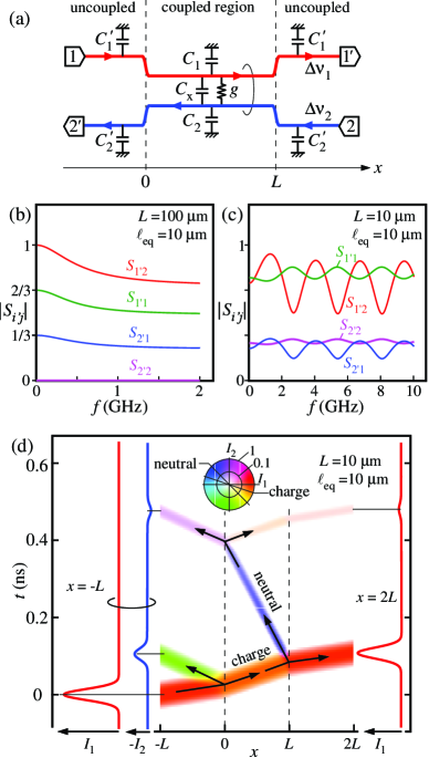
Figure 3: (a) Possible experimental setup for transmission and reflection measurements through the coupled region of length $L$. Plots in (b)-(d) are obtained with $\Delta\nu_{1}=1$, $\Delta\nu_{2}=-1/3$, $\bar{C}_{1}=\bar{C}_{2}=\bar{C}_{1}^{\prime}=\bar{C}_{2}^{\prime}=$ 0.1 nF/m, $\bar{C}_{\mathrm{x}}=$ 0.4 nF/m, and $\ell_{\mathrm{eq}}=$ 10 $\mu$m (corresponding to $g=$ 1.9 S/m). (b) and (c) Magnitude of the scattering matrix element $\left|S_{i^{\prime}j}\right|$ as a function of frequency $f$ for a long channel with $L$ = 100 $\mu$m in (b) and short channel with $L$ = 10 $\mu$m in (c). (d) Space ($x$) - time ($t$) evolution of the current profiles $I_{1}\left(x,t\right)$ and $I_{2}\left(x,t\right)$. A current pulse $I_{1}\left(t\right)$ (the leftmost trace) is injected at $x=-L$, and resulting currents, $I_{1}\left(x,t\right)$ and $I_{2}\left(x,t\right)$, are shown. In the central color plot, a specific color scale is used: orange for the charge mode, blue for the neutral mode, red for the uncoupled channel 1, and green or purple for the uncoupled channel 2. Transmitted current $I_{1}\left(t\right)$ at $x=2L$ (the rightmost trace) and reflected current$-I_{2}\left(t\right)$ at $x=-L$ (the second-left trace) also are shown.

The transport eigenmodes can be studied experimentally by investigating transmission and reflection characteristics of an interaction region with length $L$, as shown in Fig. 3(a) Bocquillon-NatCom2013 . Here, we focus on the fractional case of $\nu=2/3$, while similar results are expected for other cases. Current can be excited from ports 1 or 2, and the output current can be measured at ports 1^′ and 2^′. The intrachannel interaction in the uncoupled regions is parametrized with effective capacitances $\bar{C}_{1}^{\prime}$ and $\bar{C}_{2}^{\prime}$ (geometric capacitance $C_{c}^{\prime}$ and the density of states). The scattering matrix element $S_{i^{\prime}j}$ from input port $j$ to output port $i^{\prime}$ can be derived by using the eigenmodes in the interacting region ($\tilde{I}_{\mathrm{I}}$, $\tilde{I}_{\mathrm{II}}$, $k_{\mathrm{I}}$, and $k_{\mathrm{II}}$ derived in the previous section) and current conservation at the boundaries. By using the complex phases $\phi_{\mathrm{I}}=k_{\mathrm{I}}L$ and $\phi_{\mathrm{II}}=k_{\mathrm{II}}L$ acquired in the interacting region, the scattering matrix is written as

$$\mathbf{S} = \frac{1}{1-\text{ }\tilde{I}_{\mathrm{I}}\text{ }\tilde{I}_{\mathrm{II}}e^{i\phi_{\mathrm{I}}}e^{-i\phi_{\mathrm{II}}}}\times$$ (23)

$$\left(\begin{array}[]{cc}e^{i\phi_{\mathrm{I}}}\left(1-\tilde{I}_{\mathrm{I}}\text{ }\tilde{I}_{\mathrm{II}}\right)\text{ }&\tilde{I}_{\mathrm{II}}\left(1-e^{i\phi_{\mathrm{I}}}e^{-i\phi_{\mathrm{II}}}\right)\\ \tilde{I}_{\mathrm{I}}\left(1-e^{i\phi_{\mathrm{I}}}e^{-i\phi_{\mathrm{II}}}\right)&e^{-i\phi_{\mathrm{II}}}\left(1-\tilde{I}_{\mathrm{I}}\text{ }\tilde{I}_{\mathrm{II}}\right)\text{ }\end{array}\right).$$

First, we consider the dc characteristics with this $S$ matrix. For the $\nu=2/3$ case ($m=-3$), at the dc limit ($\omega\rightarrow 0$), eigenmodes with the characteristics of Eqs. (15) and (III) are well approximated to the pure charge mode with $\tilde{I}_{\mathrm{I}}=-1/3$ and $k_{\mathrm{I}}\simeq 0$, and the pure neutral mode with $\tilde{I}_{\mathrm{II}}=-1$ and $k_{\mathrm{II}}\simeq-2i\frac{g}{\sigma_{1}}$. The so-called equilibration length $\ell_{\mathrm{eq}}$, defined as the decay length of the neutral mode ($\left|e^{-ik_{\mathrm{II}}\ell_{\mathrm{eq}}}\right|=1/e$) Grivnin-PRL2014 ; CJLin-PRB2019 , is related to $g$ as

$$\ell_{\mathrm{eq}}=\frac{\sigma_{1}}{2g}.$$ (24)

For a long channel much greater than $\ell_{\mathrm{eq}}$, the $S$ matrix at the dc limit is reduced to

$$\mathbf{S}_{\mathrm{dc}}\simeq\left(\begin{array}[]{cc}2/3&-1\\ \text{ }-1/3&0\end{array}\right),$$ (25)

which indicates the current partition from port 1 to port 1^′ with the transmission factor 2/3 and to port 2^′ with the reflection factor 1/3 ($-S_{2^{\prime}1}$ as the polarity is defined as positive for a right-moving current).

For high-frequency transport with finite $\xi^{\prime\prime}$, mode II represents the quasi-neutral mode propagating to the left, and $k_{\mathrm{II}}$ has a significantly large negative imaginary part. By using a sufficiently long channel with $\left|e^{-i\phi_{\mathrm{II}}}\right|\ll 1$, Eq. (23) can be approximated to

$$\mathbf{S}\simeq\left(\begin{array}[]{cc}e^{i\phi_{\mathrm{I}}}\left(1-\tilde{I}_{\mathrm{I}}\text{ }\tilde{I}_{\mathrm{II}}\right)&\text{ }\tilde{I}_{\mathrm{II}}\\ \text{ }\tilde{I}_{\mathrm{I}}&e^{-i\phi_{\mathrm{II}}}\left(1-\tilde{I}_{\mathrm{I}}\text{ }\tilde{I}_{\mathrm{II}}\right)\end{array}\right).$$ (26)

At this limit, $\tilde{I}_{\mathrm{I}}$ and $\tilde{I}_{\mathrm{II}}$ can be determined directly from $S_{2^{\prime}1}$ and $S_{1^{\prime}2}$, respectively, and $k_{\mathrm{I}}$ and $k_{\mathrm{II}}$ can be determined from the phase factor in $S_{1^{\prime}1}$ and $S_{2^{\prime}2}$, respectively. Figure 3(b) shows $\left|S_{i^{\prime}j}\right|$ as a function of frequency $f$ for channel length $L$ = 100 $\mu$m ($\gg$ $\ell_{\mathrm{eq}}$ = 10 $\mu$m), where the eigenmodes at higher frequency deviate from the values at the dc limit. In contrast, when the channel length is much shorter with $\left|e^{i\phi_{\mathrm{I}}}e^{-i\phi_{\mathrm{II}}}\right|\sim 1$, the scattering matrix elements in Eq. (23) oscillate with the factor $e^{i\phi_{\mathrm{I}}}e^{-i\phi_{\mathrm{II}}}$ that arises from the plasmon interference of the two modes. Such interference can be seen in Fig. 3(c), where the channel length $L$ = 10 $\mu$m is set equal to $\ell_{\mathrm{eq}}$. Observation of the interference pattern can be used to identify all parameters in the plasmon model.

V Time-domain experiment

One can investigate the eigenmodes by using time-domain experiments Kamata-NatNano2014 ; Hashisaka-NatPhys2017 ; CJLin . For example, by using the same device structure as that shown in Fig. 3(a), a sharp current pulse can be introduced to port 1 and the resulting currents at ports 1’ and 2’ can be measured with time-resolved detectors. Such an experiment is simulated in Fig. 3(d), where non-interacting channels ($-L<x<0$ and $L<x<2L$) are attached to the interacting region of length $L$ ($0<x<L$). By applying a current pulse in the form of $I_{1}(t)$ at $x=-L$ as shown in the leftmost trace, the current distributions $I_{1}(x,t)$ and $I_{2}(x,t)$ can be calculated using Eq. (5). Note that the calculus of finite differences in space and time is problematic for this equation. Instead, we considered a periodic pulse with a long period, and the scattering matrix of Eq. (23) is used for each frequency component in the Fourier spectrum of the incident wave. The space-time solution is obtained by using the inverse Fourier transform.

The current distributions are plotted in a specific color scale with hue for the mode $\left(I_{1},I_{2}\right)$ and brightness for the magnitude in a logarithmic scale. One can see that the incident charge packet is fractionalized into different modes (colors) at $x=0$ and $x=L$. The model predicts that the transmitted current $I_{1}(t)$ at $x=2L$ (the rightmost trace) and the reflected current $-I_{2}(t)$ at $x=-L$ (the second trace from the left) should be obtained experimentally. One can investigate the transport eigenmodes by analyzing the amplitude and the time-of-flight of the fractionalized wave packets.

VI Summary

We have provided a plasmon model for two chiral edge channels in the presence of Coulomb interaction and disorder-induced tunneling by using a formulation in the incoherent regime. This can be used to systematically understand the transport characteristics of various cases, including copropagating integer channels at $\nu=2$ and counterpropagating integer/fractional channels at $\nu=2/3$. We have proposed two experimental schemes. These would use frequency- and time-domain measurements to investigate the transmission and reflection characteristics of a coupling region with a finite length. Particularly, when the coupling length is comparable to or shorter than the equilibration length, rich characteristics associated with the fractionalization at the boundaries are expected. While representative cases with $\nu=2$ and 2/3 are considered in this study, the model can be extended to more complicated quantum Hall channels (more than two channels) and other topological systems with multiple channels TopoQC-Nayak08 ; Polkovnikov-RMP2011 ; BookBernevig . This may be useful in identifying an appropriate and effective model for edge reconstructions from several candidates Beenakker-PRL90 ; Meir-PRL94 .

- (1) Z. F. Ezawa, Quantum Hall Effects: Recent Theoretical and Experimental Developments, 3rd edition, (World Scientific, Singapore, 2013).
- (2) X-G Wen, Quantum Field Theory of Many-body Systems (Oxford Univ. Press, 2004).
- (3) T. Giamarchi, Quantum Physics in One Dimension (Oxford Univ. Press, 2004).
- (4) E. Bocquillon et al., Separation of neutral and charge modes in one-dimensional chiral edge channels. Nat. Commun. 4, 1839 (2013).
- (5) H. Inoue, A. Grivnin, N. Ofek, I. Neder, M. Heiblum, V. Umansky, and D. Mahalu, Charge fractionalization in the integer quantum Hall effect, Phys. Rev. Lett. 112, 166801 (2014).
- (6) M. Hashisaka, N. Hiyama, T. Akiho, K. Muraki, and T. Fujisawa, Waveform measurement of charge- and spin-density wavepackets in a chiral Tomonaga-Luttinger liquid, Nat. Phys. 13, 559 (2017).
- (7) A. Bid, N. Ofek, M. Heiblum, V. Umansky, and D. Mahalu, Shot noise and charge at the 2/3 composite fractional quantum Hall state, Phys. Rev. Lett. 103, 236802 (2009).
- (8) R. Sabo, I. Gurman, A. Rosenblatt, F. Lafont, D. Banitt, J. Park, M. Heiblum, Y. Gefen, V. Umansky, D. Mahalu, Edge reconstruction in fractional quantum Hall states, Nat. Phys. 13, 491 (2017).
- (9) F. Lafont, A. Rosenblatt, M. Heiblum, V. Umansky, Counter-propagating charge transport in the quantum Hall effect regime, Science 363, 54 (2019).
- (10) H. Kamata, T. Ota, K. Muraki, and T. Fujisawa, Voltage-controlled group velocity of edge magnetoplasmon in the quantum Hall regime, Phys. Rev. B 81, 085329 (2010).
- (11) C. Altimiras, H. le Sueur, U. Gennser, A. Cavanna, D. Mailly, and F. Pierre, Non-equilibrium edge-channel spectroscopy in the integer quantum Hall regime. Nat. Phys. 6, 34 (2010).
- (12) H. Kamata, N. Kumada, M. Hashisaka, K. Muraki, and T. Fujisawa, Fractionalized wave packets from an artificial Tomonaga-Luttinger liquid. Nat. Nanotech. 9, 177 (2014).
- (13) K. Itoh, R. Nakazawa, T. Ota, M. Hashisaka, K. Muraki and T. Fujisawa, Signatures of a Nonthermal Metastable State in Copropagating Quantum Hall Edge Channels. Phys. Rev. Lett. 120, 197701 (2018).
- (14) Y. Ji, Y. C. Chung, D. Sprinzak, M. Heiblum, D. Mahalu, and H. Shtrikman, An electronic Mach-Zehnder interferometer, Nature 422, 415 (2003).
- (15) E. Berg, Y. Oreg, E. A. Kim, and F. von Oppen, Fractional charges on an integer quantum Hall edge. Phys. Rev. Lett. 102, 236402 (2009).
- (16) C. L. Kane and M. P. A. Fisher, Contacts and edge-state equilibration in the fractional quantum Hall effect. Phys. Rev. B 52, 17393 (1995).
- (17) C. L. Kane, M. P. A. Fisher, and J. Polchinski, Randomness at the Edge: Theory of quantum Hall transport at filling = 2/3, Phys. Rev. Lett. 72, 4129 (1994).
- (18) A. Grivnin, H. Inoue, Y. Ronen, Y. Baum, M. Heiblum, V. Umansky, and D. Mahalu, Non-equilibrated counter propagating edge modes in the fractional quantum Hall regime, Phys. Rev. Lett. 113, 266803 (2014)
- (19) C. J. Lin, R. Eguchi, M. Hashisaka, T. Akiho, K. Muraki, and T. Fujisawa, Charge equilibration in integer and fractional quantum Hall edge channels in a generalized Hall-bar device, Phys. Rev. B 99, 195304 (2019).
- (20) C. J. Lin, M. Hashisaka, T. Akiho, K. Muraki, and T. Fujisawa, Quantized charge fractionalization at quantum Hall Y junctions in the disorder dominated regime, Nature Commun. 12, 131 (2021).
- (21) I. Safi, and H. J. Schulz, Transport in an inhomogeneous interacting one-dimensional system, Phys. Rev. B 52, R17040(R) (1995).
- (22) I. Safi, A dynamic scattering approach for a gated interacting wire, Eur. Phys. J. B 12, 451 (1999).
- (23) I. V. Protopopov, T. Gefen, and A. D. Mirlin, Transport in a disordered = 2/3 fractional quantum Hall junction, Ann. Phys. 385, 287 (2017).
- (24) M. Hashisaka, K. Washio, H. Kamata, K. Muraki, and T. Fujisawa, Distributed electrochemical capacitance evidenced in high-frequency admittance measurements on a quantum Hall device, Phys. Rev. B 85, 155424 (2012).
- (25) A. H. MacDonald, Edge states in the fractional-quantum-Hall effect regime, Phys. Rev. Lett. 64, 220 (1990).
- (26) X. G. Wen, Electrodynamical properties of gapless edge excitations in the fractional quantum Hall states, Phys. Rev. Lett. 64, 2206 (1990).
- (27) C. Nosiglia, J. Park, B. Rosenow, and Y. Gefen, Incoherent transport on the = 2/3 quantum Hall edge, Phys. Rev. B 98, 115408 (2018).
- (28) M. Hashisaka and T. Fujisawa, Tomonaga-Luttinger-liquid nature of edge excitations in integer quantum Hall edge channels, Reviews in Physics 3, 32 (2018).
- (29) J. Gabelli, G. Feve, T. Kontos, J. M. Berroir, B. Placais, D. C. Glattli, B. Etienne, Y. Jin, and M. Buttiker, Relaxation Time of a Chiral Quantum R-L Circuit, Phys. Rev. Lett. 98, 166806 (2007).
- (30) C. Spånslätt, J. Park, Y. Gefen, A. D. Mirlin, Topological Classification of Shot Noise on Fractional Quantum Hall Edges, Phys. Rev. Lett 123, 137701 (2019).
- (31) J. Park, A. D. Mirlin, B. Rosenow, and Y. Gefen, Noise on complex quantum Hall edges: Chiral anomaly and heat diffusion, Phys. Rev. B 99, 161302(R) (2019).
- (32) C. Nayak, S. H. Simon, A. Stern, M. Freedman and S. Das Sarma, Non-Abelian anyons and topological quantum computation, Rev. Mod. Phys. 80, 1083 (2008).
- (33) A. Polkovnikov, K. Sengupta, A. Silva, and M. Vengalattore, Nonequilibrium dynamics of closed interacting quantum systems, Rev. Mod. Phys. 83, 863 (2011).
- (34) B. A. Bernevig, Topological Insulators and Topological Superconductors, (Princeton Univ. Press 2013).
- (35) C. W. J. Beenakker, Edge channels for the fractional quantum Hall effect. Phys. Rev. Lett. 64, 216 (1990).
- (36) Y. Meir, Composite edge states in the = 2/3 fractional quantum Hall regime. Phys. Rev. Lett. 72, 2624 (1994).