DiffAqua: A Differentiable Computational Design Pipeline for Soft Underwater Swimmers with Shape Interpolation

Abstract.

The computational design of soft underwater swimmers is challenging because of the high degrees of freedom in soft-body modeling. In this paper, we present a differentiable pipeline for co-designing a soft swimmer’s geometry and controller. Our pipeline unlocks gradient-based algorithms for discovering novel swimmer designs more efficiently than traditional gradient-free solutions. We propose Wasserstein barycenters as a basis for the geometric design of soft underwater swimmers since it is differentiable and can naturally interpolate between bio-inspired base shapes via optimal transport. By combining this design space with differentiable simulation and control, we can efficiently optimize a soft underwater swimmer’s performance with fewer simulations than baseline methods. We demonstrate the efficacy of our method on various design problems such as fast, stable, and energy-efficient swimming and demonstrate applicability to multi-objective design.

Figure 1. In this example, we co-design a swimmer’s geometry and controller for position-keeping in running water (blue arrows in upper middle and upper right). The blue and red spheres indicate the desired and actual position of the swimmer. The swimmer’s geometric design weights are initialized as the average of 12 base shapes with the Wasserstein distance metric shown in gray (left). After optimization, the final geometric design weights of each base shape are shown in orange (left). With the initial shape and actuator locations (upper middle) and the initial controller (lower middle), the position-keeping performance is poor, as indicated by the large distance between the red and blue dots. With the optimized shape and actuator locations (upper right) and the optimized controller (lower right), performance is markedly improved, i.e., blue and red are closer together.

1. Introduction

Designing bio-inspired underwater swimmers has long been an exciting interdisciplinary research problem for biologists and engineers (Triantafyllou and Triantafyllou, 1995; Marchese et al., 2014; Katzschmann et al., 2018; Berlinger et al., 2018; Fish and Lauder, 2006). Aquatic locomotive performance of underwater swimmers is governed by two interrelated aspects: the control policy responsible for coordinated actuation and the geometry by which the actuation is transformed into motion through hydrodynamic forces. While the computational co-design of geometry and control has been explored in the context of articulated rigid walking and flying robots (Zhao et al., 2020; Du et al., 2016; Pathak et al., 2019; Ha, 2019), the co-design of geometry and control of a soft robot consisting of substantially deformable materials has been sparsely studied. Since a soft robot is governed by continuum physics with many more degrees of freedom (DOFs), existing methods are not readily transferable to soft robotic design problems. Optimizing over all degrees of freedom of an infinite-dimensional continuum elastic body is computationally intractable, even when approximated with a large number of discrete elements. Lower-dimensional geometric representations are needed to allow for efficient shape exploration without sacrificing expressiveness.

To remedy the lack of an intuitive and low-dimensional design space suitable for soft underwater swimmers, we propose representing a soft swimmer’s shape and actuators as probability distributions in 3D space and interpolate between designs with optimal transport (Rubner et al., 2000). Given a set of base shapes representing swimmer archetypes, we define a vector space spanned by these shapes according to the Wasserstein distance metric (Solomon et al., 2015). Such a representation of the soft swimmer’s design space brings a few key benefits. First, it allows for each design to be represented as a low-dimensional Wasserstein barycentric weight vector. Second, and more importantly, this interpolation procedure is differentiable (Bonneel et al., 2016), enabling gradient-based optimization algorithms for fast exploration of the design space. We further combine this design space with a differentiable simulator (Du et al., 2021) and control policy, creating a full pipeline for co-optimizing the body and brain of soft swimmers using gradient-based optimization algorithms.

We evaluate our co-optimization pipeline on a set of soft swimmer design problems whose objectives include forward swimming, stable swimming under opposing flows, and energy conservation. We further demonstrate the pipeline’s applicability to multi-objective design and the generation of Pareto fronts. We show that our algorithm converges significantly faster than gradient-free optimization algorithms (Hansen et al., 2003) and strategies that alternate between optimizing geometric design and control.

In this paper, we contribute:

• a low-dimensional differentiable design space parametrizing the shape and actuation of soft underwater swimmers with the Wasserstein distance metric,

• a differentiable pipeline for co-optimizing the geometric design and controller of a soft swimmer concurrently, and

• demonstrations of this algorithm on a set of bio-inspired single- and multi-objective underwater swimming tasks.

2. Related Work

Our approach builds upon recent and seminal work in differentiable simulation, soft robot and character control, computational co-design of robots, and shape parametrizations.

Differentiable simulation

Differentiable simulation allows for the direct computation of the gradients of continuous parameters affecting the system performance, such as control, material, and geometric parameters. Gradients computed from differentiable simulation can be directly fed into numerical optimization algorithms, immediately unlocking applications such as system identification, computational control, and design optimization. Differentiable simulation has a rich history in robotics and physically-based animation across various domains, including rigid-body dynamics (Popović et al., 2003; Degrave et al., 2019; Belbute-Peres et al., 2018; Geilinger et al., 2020), fluid dynamics (Holl et al., 2020; McNamara et al., 2004; Schenck and Fox, 2018) and cloth physics with rigid coupling (Liang et al., 2019; Qiao et al., 2020). In cases where manually deriving gradients is difficult, automatic differentiation frameworks (Giftthaler et al., 2017; Hu et al., 2020) or learned, approximate models (Li et al., 2019; Sanchez-Gonzalez et al., 2020; Chen et al., 2018) have been employed. Most related to our work are differentiable simulation methods for soft bodies (Hu et al., 2019; Hahn et al., 2019; Du et al., 2021; Huang et al., 2021). We build upon the work of Du et al. (2021), which proposes a differentiable projective dynamics framework capable of implicit integration.

Dynamic soft robot and character control

Soft robotic control is traditionally more difficult than rigid robotic control, since the infinite-dimensional state spaces of soft robots are difficult to computationally reason about. Previous papers (Geijtenbeek et al., 2013; Won and Lee, 2019) demonstrated learning general controllers for articulated, rigid-body walking robots in a variety of forms. Tan et al. (2011) explored model-based control optimization of articulated rigid swimmers in an environment coupled with fluid. Control using model-free reinforcement learning for systems with solid-fluid coupling has been studied in Ma et al. (2018). Simplified dynamical models which treat soft tendril structures compactly and accurately as rod-and-spring-like structures have allowed for the natural adoption of modern control algorithms like those used for articulated rigid robots (Marchese et al., 2016; Della Santina et al., 2018; Katzschmann et al., 2019a). Grzeszczuk and Terzopoulos (1995) proposed representing the actuators of swimmers with a simplified biomechanical model and automatically generating their controllers. There are also works, such as Hecker et al. (2008), synthesizing animation independent of character morphology for the purpose of downstream retargeting, with the motion described by familiar posing and key-framing methods. More general approaches (Barbič and Popović, 2008; Barbič et al., 2009; Thieffry et al., 2018; Spielberg et al., 2019; Katzschmann et al., 2019b) present dimensionality reduction strategies for soft robots to compact representations used in model-based control. Most similar to our work are the approaches of Hu et al. (2019) and Min et al. (2019). In Hu et al. (2019), a differentiable soft-body simulator is coupled with parametric neural network controllers. By tracking the positions and velocities of manually specified regions as control inputs, a loss function measuring the forward progress in robot locomotion is directly backpropagated to control parameters, enabling efficient model-based control optimization via gradient descent. Min et al. (2019) present model-free control of soft swimmers using reinforcement learning with similar handcrafted features. Our approach for control optimization is similar to the model-based optimization framework of Hu et al. (2019), but instead of considering legs and crawlers, we optimize underwater swimmers. Our work further distinguishes itself from prior art through the realization of the non-trivial co-optimization of shape and control of soft underwater swimmers.

Computational robot co-design

Much of the existing work on the co-design of rigid robots has focused on the interplay between geometric, inertial and control parameters. Megaro et al. (2015); Schulz et al. (2017b) explored the interactive design of robot control and geometry, in which CAD-like front-ends guided human-in-the-loop, simulation-driven control and design optimization. Wampler and Popović (2009); Spielberg et al. (2017); Ha et al. (2017) presented algorithms for co-optimizing geometric and inertial parameters of robots with open-loop controllers; Schaff et al. (2019); Ha (2019) extended these ideas to the space of closed-loop neural network controllers via reinforcement learning approaches. Du et al. (2016) presented a method for co-optimizing the control and geometric parameters for optimal multicopter performance. Sims (1994) models the morphology as a graph and co-optimizes it with control using an evolutionary strategy. In each of the approaches described above, the geometric representations are simple. Each robotic link is parameterized by no more than a handful of geometric parameters, substantially limiting the morphological search. More complex representations are used in the works by Ha et al. (2018); Wang et al. (2018); Zhao et al. (2020), presenting algorithms for searching over various robot topologies. These techniques lead to more geometrically and functionally varied robots; however, this discrete search space cannot be directly optimized by the continuous optimization approaches to which differentiable simulation lends itself.

Computational co-design of soft robots has been more sparsely explored. Cheney et al. (2014); Corucci et al. (2016); Van Diepen and Shea (2019) presented heuristic search algorithms for searching over soft robotic topology and control, including swimmers in the case of Corucci et al. (2016). These sampling-based approaches focus on geometry and (discrete) materiality, typically leaving actuation as open-loop, pre-programmed cyclic patterns. Contrasted with these approaches are those of Hu et al. (2019); Spielberg et al. (2019), which exploit system gradients to co-optimize over closed-loop control, observation models, and spatially varying material parameters, but not geometry. Our approach combines advantages of both lines of research, relying on the differentiable simulation for fast gradient-based co-optimization of neural network control and complex geometry.

Shape interpolation

Many bases for shape representations have been proposed over the years for applications in shape analysis. Geometrically-based spaces (Ovsjanikov et al., 2012; Lewis et al., 2014; Baek et al., 2015; Solomon et al., 2015; Schulz et al., 2017a; Bonneel et al., 2016) parameterize shape collections based on intrinsic geometric metrics computed across a data set; learning-based spaces (Bronstein et al., 2011; Averkiou et al., 2014; Fish et al., 2014; Yang et al., 2019; Mo et al., 2019; Park et al., 2019), by contrast, learn parametrizations based on statistical features of that dataset and can also easily incorporate non-geometric information (such as labels). In this work, we opt for the geometrically-based convolutional Wasserstein basis (Solomon et al., 2015), which interpolates between meshes using the Wasserstein distance. This basis smoothly interpolates between shapes with “as few” in-between modifications as necessary, keeping our mesh parametrizations well-behaved and minimizing the chance of artifacts that might cause difficulties in simulation. This continuous and differentiable basis makes it amenable to continuous co-optimization.

3. System Overview

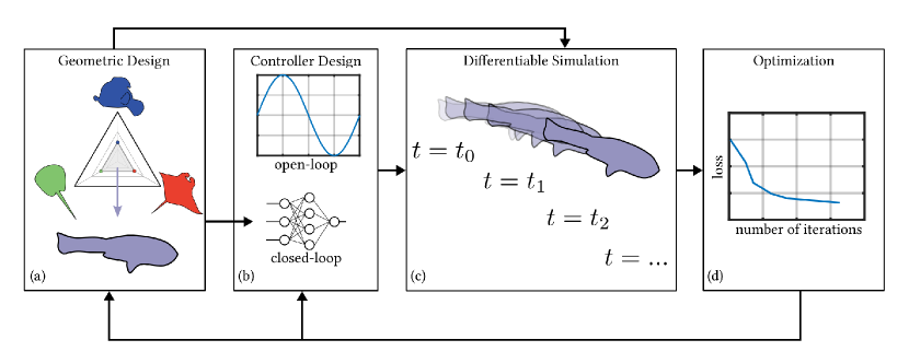
Figure 2. In our computational design pipeline, we begin with (a) the shape and actuator design using the Wasserstein distance to interpolate smoothly between base shapes and between actuators. Given a set of base shapes by the user, we initialize the shape parametrization by assigning equal weights to all bases. (b) Next, we consider the controller design for two cases: an open-loop controller and a closed-loop controller. (c) Given this initial shape, actuators, and controller, we simulate the design using a differentiable simulator to evaluate its performance. (d) Finally, we take advantage of the differentiability of our framework to compute the gradients of a given objective with respect to geometry and control parameters simultaneously. These gradients are used in a gradient descent optimizer to concurrently adapt the geometric and control design parameters.

Our design optimization procedure starts with a collection of base shapes from which to build a geometric design space using the Wasserstein distance metric. Each base design also specifies a multivariate normal distribution for each of its actuators. For our bio-inspired exploration of swimmers, we have selected base shapes inspired by nature (Sec. 4), e.g., sharks, manta rays, and goldfish. Next, the user specifies a controller which is either an open-loop sinusoidal signal or a neural network. The state observations of the closed-loop neural network controller are defined by the user (Sec. 5). The user then evaluates the soft swimmer via differentiable simulation (Sec. 6), which returns both the swimmer’s performance and its gradients with respect to geometric design and control parameters. Finally, we embed both the design space and the differentiable simulator in a gradient-based optimization procedure, which co-optimizes both the geometric design and the controller until convergence (Sec. 7), closing our design loop. We present the overview of our method in Fig. 2.

4. Geometric Design

Our soft swimmer’s geometric design consists of two parts: its volumetric shape and its actuator locations. This section explains our differentiable parameterization of this geometric design space. The key idea is to represent geometric designs as probability density functions and generate novel swimmers by interpolating the probability density functions of the base designs. After the design space has been parametrized, any swimmer in this space can be represented compactly by low-dimensional discrete and continuous parameters.

4.1. Shape Design

Given a set of user-defined base shapes, we interpolate between these bases with the Wasserstein distance metric to form a continuous and differentiable shape space. The reason behind this choice is twofold. First, the Wasserstein barycentric interpolation encourages smooth, plausible intermediate results even between shapes with substantially different topology (Solomon et al., 2015), which is common in underwater creatures. Second, efficient numerical solutions exist for solving Wasserstein barycenters, and their gradients are also readily available (Solomon et al., 2015; Bonneel et al., 2016). These two features make Wasserstein distance a proper choice for building a fully differentiable shape design space for soft swimmers.

Formally, we consider the designs of our soft swimmers to be embedded in an axis-aligned bounding box $\Omega\subseteq\mathcal{R}^{d}$, where $d=2$ or $3$ is the dimension. Without loss of generality, we rescale $\Omega$ uniformly and shift it so that it has unit volume and is centered at the origin of $\mathcal{R}^{d}$. We use $d_{E}:\Omega\times\Omega\rightarrow\mathcal{R}_{+}$ to denote the Euclidean distance function, $\mathcal{P}(\Omega)$ the space of probability measures on $\Omega$, and $\mathcal{P}(\Omega\times\Omega)$ the space of probability measures on $\Omega\times\Omega$.

For any probability measure $P\in\mathcal{P}(\Omega)$, we define the following set $S\subseteq\Omega$ based on $P$’s probability density function $p$ to represent a soft swimmer’s shape:

(1) $$S(p)=\{\bm{x}|p(\bm{x})\geq 0.5\sup_{\bm{x}\in\Omega}p(\bm{x})\}.$$

In other words, a soft swimmer’s shape occupies the volumetric region where the probability density is over half the peak density. Similarly, the surface of the shape, which is primarily used for computing hydrodynamic forces and visualizing the shape, is defined as follows:

(2) $$\partial S(p)=\{\bm{x}|p(\bm{x})=0.5\sup_{\bm{x}\in\Omega}p(\bm{x})\}$$

Shape bases

Although these probability density functions provide us a design space that can express almost all possible soft swimmer shape designs, its infinite degrees of freedom makes design optimization computationally challenging. Moreover, the probability measure space includes many physically implausible shapes that would be rejected instantly by a human user. To encourage findings of physically plausible swimmers from a low-dimensional shape space, we build a library consisting of $m$ soft swimmers designed by human experts and define the shape space as the vector space spanned from these designs. Specifically, let $S_{1},S_{2},\cdots,S_{m}\subseteq\Omega$ be the $m$ shapes in the library, we define the probability density function $p_{i}$ for $i=1,2,\cdots,m$ as follows:

(3) $$p_{i}(\bm{x})=\begin{cases}\frac{1}{|S_{i}|}&\text{if }\bm{x}\in S_{i},\\ 0&\text{otherwise.}\end{cases}$$

Furthermore, we use $P_{i}$ to refer to the corresponding probability measures induced by $p_{i}$, which serve as the basis for shape interpolation.

Shape interpolation

With all probability measures $P_{i}$ at hand, we consider the shape space parametrized by a weight vector $\bm{\alpha}\in\mathcal{R}^{m}$ in the probability simplex $\{\bm{\alpha}|\alpha_{i}\geq 0,\sum_{i}\alpha_{i}=1\}$. Specifically, given a weight vector $\bm{\alpha}$, we compute the Wasserstein barycenter $P(\bm{\alpha})$, which can be interpreted as a weighted average of $P_{1},P_{2},\cdots,P_{m}$ (Solomon et al., 2015):

(4) $$P(\bm{\alpha})=\underset{P\in\mathcal{P}(\Omega)}{\arg\min}\sum_{i}\alpha_{i}\mathcal{W}_{2}^{2}(P,P_{i}).$$

Here, $\mathcal{W}_{2}(\cdot,\cdot):\mathcal{P}(\Omega)\times\mathcal{P}(\Omega)\rightarrow\mathcal{R}_{+}$ is the 2-Wasserstein distance:

(5) $$\mathcal{W}_{2}(P,Q)=\left[\inf_{\pi\in\Pi(P,Q)}\iint_{\Omega\times\Omega}d_{E}^{2}(\bm{x},\bm{y})d\pi(\bm{x},\bm{y})\right]^{\frac{1}{2}}$$

where $\Pi(P,Q)$ is the set of transportation maps from probability measure P to Q:

(6) $$\Pi(P,Q)=\{\pi\in\mathcal{P}(\Omega\times\Omega)|\pi(\cdot,\Omega)=P,\pi(\Omega,\cdot)=Q\}.$$

In short, for each weight vector $\bm{\alpha}$, we compute the Wasserstein barycenter $P(\bm{\alpha})$ and use its probability density function to define a new shape $S(\bm{\alpha})$, with some abuse of notation $S$. This way, we establish an isomorphic mapping from the probability simplex to the shape space. Exploring the shape space is then equivalent to navigating the continuous, low-dimensional probability simplex.

4.2. Actuator Design

In this work, we use the contractile muscle fiber model introduced by Min et al. (2019) to actuate soft swimmers. Like the shape interpolation scheme above, users first specify the geometric representation of actuators for all soft swimmers in the library. Then, our method interpolates between them to obtain actuators for shapes at Wasserstein barycenters.

Actuator representation

For a given soft swimmer, we define its actuators by a set of discrete and continuous labels. Each actuator has one discrete parameter denoting its category and a small number of continuous parameters defining its location, size, and orientation. The actuator categories supported in this work include “left fin”, “right fin”, and “caudal fin”, which indicate the actuator’s rough location (Fig. 5). Each soft swimmer has at most one actuator for each category. The actuator’s continuous parameters represent its geometric design with a multivariate normal distribution $\mathcal{N}(\bm{\mu},\bm{\Sigma})$ where $\bm{\mu}\in\mathcal{R}^{d}$ and $\bm{\Sigma}\in\mathcal{R}^{d\times d}$ are its mean and variance. Similar to the shape function $S$, the actuator’s shape $A$ is defined by the locations whose probability density is over half of the peak density from $\mathcal{N}(\bm{\mu},\bm{\Sigma})$:

(7) $$A^{c}_{S}(\bm{\mu},\bm{\Sigma})=B(\{\bm{x}|\exp(-\frac{1}{2}(\bm{x}-\bm{\mu})^{\top}\bm{\Sigma}^{-1}(\bm{x}-\bm{\mu}))\geq 0.5\})\cap S.$$

Here, $A^{c}_{S}$ stands for the volumetric region occupied by an actuator of category $c$ in a soft swimmer whose shape is $S$, and $B:\Omega\rightarrow\Omega$ is a function that takes as input a $d$-dimensional ellipsoid and returns the minimum bounding box whose directions are aligned with the principal axes of the ellipsoid (Fig. 3). Note that the intersection with $S$ ensures the actuator stays in the interior of $S$. With some abuse of notation, we use $A^{c}_{P}$ and $A^{c}_{\bm{\alpha}}$ to denote an actuator of category $c$ in a soft swimmer defined by a probability measure $P$ or the Wasserstein barycentric interpolation with a weight vector $\bm{\alpha}$, respectively. When designing a soft swimmer $S_{i}$ in the library, the human expert also specifies its actuators’ discrete and continuous parameters to obtain $\{A^{c}_{i}\}_{c}$, defined as follows:

(8) $$A^{c}_{i}=A^{c}_{S_{i}}(\bm{\mu}^{c}_{i},\bm{\Sigma}^{c}_{i})$$

where $\bm{\mu}^{c}_{i}$ and $\bm{\Sigma}^{c}_{i}$ are prespecified mean and variance for the actuators with category $c$ in shape $S_{i}$.

Actuator interpolation

We now describe how to generate actuators for a soft swimmer interpolated using the Wasserstein distance. Let $\bm{\alpha}$ be the weight vector defined above. For the soft swimmer defined by the probability measure $P(\bm{\alpha})$ and for each actuator category $c$, we define $A^{c}_{\bm{\alpha}}$ as follows:

(9) $$A^{c}_{\bm{\alpha}}=A^{c}_{S(\bm{\alpha})}(\bm{\mu}^{c}_{\bm{\alpha}},\bm{\Sigma}^{c}_{\bm{\alpha}})$$

where $\bm{\mu}^{c}_{\bm{\alpha}}$ and $\bm{\Sigma}^{c}_{\bm{\alpha}}$ are continuous parameters computed as follows:

(10) $$\bm{\mu}^{c}_{\bm{\alpha}}= ~{}\text{LinearInterpolation}(\bm{\alpha},\bm{\mu}^{c}_{i}),$$

(11) $$\bm{\Sigma}^{c}_{\bm{\alpha}}= ~{}(\bm{R}^{c})^{\top}\bm{S}^{c}\bm{R}^{c},$$

(12) $$\bm{R}^{c}= ~{}\text{RotationalInterpolation}(\bm{\alpha},\bm{R}^{c}_{i}),$$

(13) $$\bm{S}^{c}= ~{}\text{LinearInterpolation}(\bm{\alpha},\bm{S}^{c}_{i}).$$

Here, both $\bm{\mu}^{c}_{\bm{\alpha}}$ and $\bm{\Sigma}^{c}_{\bm{\alpha}}$ are defined by interpolating the means and variances of the actuators from the base shapes with the weight vector $\bm{\alpha}$. If the actuator of category $c$ is not used by the $i$-th base shape, we set the corresponding weight $\alpha_{i}$ to zero so that it is excluded from the interpolation. The mean $\bm{\mu}^{c}_{\bm{\alpha}}$ is computed by linearly interpolating between the $\bm{\mu}^{c}_{i}$. The variance matrix $\bm{\Sigma}^{c}_{\bm{\alpha}}$ is obtained by linearly interpolating the eigenvalues $\bm{S}^{c}_{i}$ and the Euler angles of the rotational matrices $\bm{R}^{c}_{i}$ from the actuator of category $c$ in the $i$-th base shapes. Note that, for simplicity, the actuators are not interpolated using the Wasserstein distance. We leave solving for the exact actuator interpolation as future work.

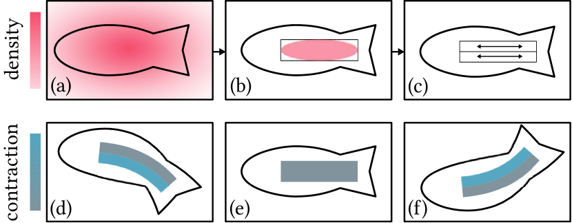
Figure 3. We explain our actuator design with a 2D fish illustration. Sec. 4: (a) We use a multivariate normal distribution to parametrize the location of the actuators. The gradient of light pink to dark pink represents the increasing probability density function. (b) The actuator’s shape is defined by the bounding box of the probability density’s isocontour at half of its peak density. We draw a black bounding box around the clipped distribution to form the actuator. Sec. 5: (c) Our actuator is divided into a pair of antagonistic muscle fibers acting in opposition. We show the extreme deformations of the fish tail in (d) the left-most position, (e) the neutral position, and (f) the right-most position. More contraction of each muscle fiber is indicated by a darker blue. The rest shape of the muscle fiber is depicted in gray.

5. Control

In this section, we first explain the actuation model built upon the actuator’s geometric design defined in the previous section. Next, we introduce two controllers for the soft underwater swimmer’s motion: an open-loop controller defined by analytic functions and a closed-loop neural network controller.

5.1. Actuation Model

As we explain in the previous section, each actuator is a cubic region defined by a clipped multivariate normal distribution. Following the muscle fiber model from previous work (Min et al., 2019; Du et al., 2021), we model each actuator as a group of parallel muscle fibers. Each muscle fiber can contract itself along the fiber direction based on the magnitude of the control signal. For the “caudal fin” actuator, the parallel muscle fibers are placed antagonistically, allowing us to actuate bilateral flapping (Fig. 3).

5.2. Open-Loop Controller

The muscles of marine animals are usually actuated periodically like waves. Inspired by this, the first controller we consider in this work is a series of sinusoidal waves:

(14) $$a(t)=a\sin(\omega t+\varphi)$$

where $t$ stands for the time and $a$, $\omega$, and $\varphi$ are the control parameters to be optimized and may vary between different actuator categories. When combined with the parallel muscle fibers in each actuator, the open-loop controller generates an oscillating motion sequence from the soft swimmer’s body.

5.3. Closed-Loop Controller

In addition to open-loop controllers, we also consider using closed-loop neural network controllers to achieve more precise control over a soft swimmer’s motion. Our neural network controller takes sensor data as input and returns control signals used to activate the actuation of the parallel muscle fibers.

Sensing

For a soft underwater swimmer in our design space, we gather position and velocity information from a swimmer’s head, center, and tail. More concretely, we first align all swimmers in the library so that their heading is along the positive $x$-axis. After this alignment, we ensure the heading of any interpolated design is also along the positive $x$-axis. We then place the head, center, and tail sensor at locations along the $x$-axis with the maximum, zero, and minimum $x$ values within the swimmer’s shape. We stack the outputs from all three sensors into a single vector and send it to the neural network controller.

Neural network controller

Our neural network controller is a standard multilayer perceptron network with two layers of $64$ neurons. We use $\tanh$ as the activation function. The input to the network includes the velocities from all three sensors and also the positional offsets from the center sensor to the head and tail sensors. Additionally, our network also takes as input a $20$-dimensional temporal encoding vector $\phi(t)$ to sense the temporally contextual information and encourage periodic control output, which is defined as follows (Vaswani et al., 2017):

(15) $$\begin{split}\phi(t)=[&\sin(2^{0}\pi\tau(t)),\sin(2^{1}\pi\tau(t)),\cdots,\sin(2^{9}\pi\tau(t)),\\ &\cos(2^{0}\pi\tau(t)),\cos(2^{1}\pi\tau(t)),\cdots,\cos(2^{9}\pi\tau(t))].\end{split}$$

Here, $\tau:\mathcal{R}_{+}\rightarrow[0,1]$ wraps the actual $t$ with a predefined period $T$: $\tau(t)=\frac{t\text{ mod }T}{T}$. We use $T=25h$ where $h$ is the time step in each experiment. We concatenate the sensor feedback and the temporal encoding as a $35$-dimensional vector, which is used as the input to the neural network controller. The neural network then outputs control signals for all actuators.

6. Differentiable Simulation

Given a soft swimmer’s geometric design and controller, we now describe how to evaluate the swimmer’s performance and gradients in a differentiable simulation environment. We build our differentiable simulator upon Min et al. (2019) and Du et al. (2021), which use projective dynamics, a fast finite element simulation method amenable to implicit integration. We consider the geometric domain $\Omega$ as the material space and the swimmer’s shape $S(p)$ as the rest shape of a deformable body. One way to forward simulate the design is to extract the surface boundary $\partial S(p)$ from the level set of its probability density function $p$, discretize $S(p)$ into finite elements, and simulate its motion by tracking its vertex locations. While this is a viable option for the forward simulation, this Lagrangian representation of the geometric design brings a few challenges for design optimization. First, whenever $S$ is updated, we need to regenerate the volumetric mesh to avoid narrow finite elements, and such a geometric processing step could be computationally expensive. Second, gradient computation depends on the exact discretization of $S(p)$, but the way to partition $S(p)$ into finite elements is not unique. Therefore, picking any specific partition may bias the gradient computation unintentionally.

Spatial and time discretization

As a result, we choose to evolve the soft swimmer’s motion with an Eulerian view based on the probability density function $p$. Specifically, we simulate the full geometric domain $\Omega$ with a spatially varying stiffness defined by $p$. For the volumetric region outside $S(p)$, we assign close-to-zero stiffness so that simulating it has a negligible effect on the soft swimmer’s motion. More formally, we consider a uniform grid that discretizes $\Omega$. Let $n$ be the number of nodes in the grid and let $\bm{q}_{i},\bm{v}_{i}\in\mathcal{R}^{dn}$ be the nodal positions and velocities at the beginning of the $i$-th time step. We simulate the grid based on the implicit time-stepping scheme:

(16) $$\bm{q}_{i+1}= \,\bm{q}_{i}+h\bm{v}_{i+1}$$

(17) $$\bm{v}_{i+1}= \,\bm{v}_{i}+h\bm{M}^{-1}[\bm{f}_{\text{int}}(\bm{q}_{i+1})+\bm{f}_{\text{ext}}]$$

where $h$ denotes the time step, $\bm{M}\in\mathcal{R}^{dn\times dn}$ is the mass matrix, and $\bm{f}_{\text{int}},\bm{f}_{\text{ext}}\in\mathcal{R}^{dn}$ are the internal and external forces applied to the $n$ nodes. As we inherit the constitutive model and the actuator model from Min et al. (2019), we skip their implementation details and focus on explaining how our spatially varying stiffness field is used to define the constitutive model. Specifically, we define a cell-wise constant Young’s modulus field $E(c)$:

(18) $$E(c)=E_{0}G(\hat{p}_{c},0.1)$$

where $c$ is the cell index, $E_{0}$ is a base Young’s modulus and $\hat{p}_{c}$ is the discretized value of $p$ in cell $c$. We further divide $\hat{p}_{c}$ by its maximum value from all cells so that $\hat{p}_{c}$ is between $0$ and $1$. $G(\cdot,0.1):[0,1]\rightarrow[0,1]$ is the Schlick’s function (Schlick, 1994),

and choosing its second argument to be $0.1$ pushes the output of $G$ towards the binary value $0$ or $1$ (see the inset). Recall that the soft swimmer’s shape is defined at locations where $p$ is at least half of the peak density, using $G(\cdot,0.1)$ encourages the soft swimmer’s body to have a Young’s modulus close to $E_{0}$. Additionally, it suppresses the volumetric region outside the swimmer to have a close-to-zero Young’s modulus so that its effect on the swimmer’s motion is negligible (Fig. 4).

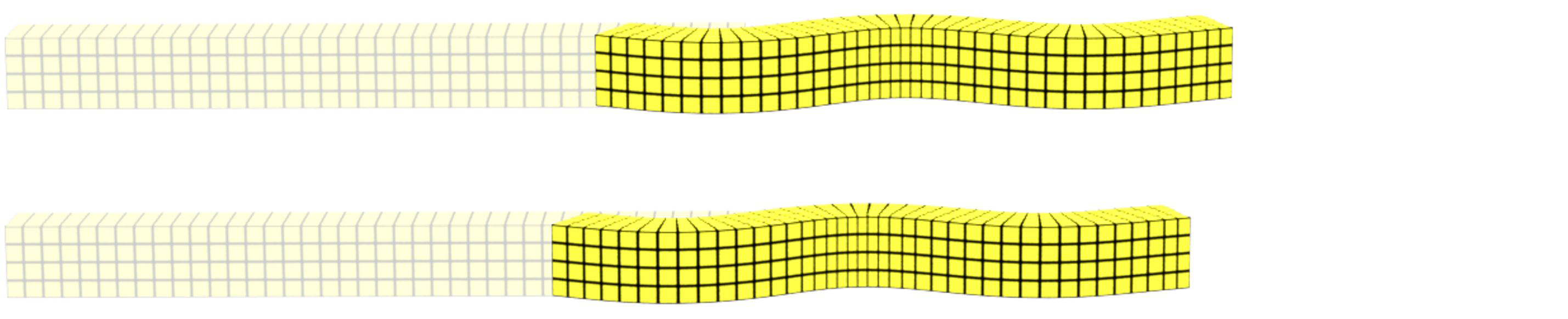
No exterior cells

Ours

Figure 4. To understand the effects of simulating a volumetric region outside a swimmer with a close-to-zero Young’s modulus, we simulate an eel without the volumetric region outside its shape (top) and compare it to our method (middle), which simulates the whole domain $\Omega$ but assigns small Young’s modulus to the volumetric region outside the eel. The relative error for each time step converges to around $6\%$ after $100$ time steps (bottom). We compute the relative error by computing the average difference between nodal positions from the two simulations and dividing it by the length of the eel.

We stress that the choice of simulating the entire domain $\Omega$ with spatially varying Young’s modulus brings us two key benefits. First, discretization is done trivially on the background grid. We avoid the expensive discretization process involving the level set of $p$, and evolving the shape design is merely updating the probability density function on the regular grid. Second, and more importantly, since a differentiable simulator provides gradients about the material stiffness, and algorithms for Wasserstein barycentric interpolation offer gradients about the probability density function (Bonneel et al., 2016), formulating the material stiffness as a function of the probability density connects the gradients from shape design and simulation into a uniform pipeline seamlessly.

Hydrodynamics

To efficiently mimic the interaction between the water and the swimmer, we develop a hydrodynamics formulation based on Min et al. (2019). In this model, the thrust and drag forces are computed on each quadrilateral from the swimmer’s surface mesh after discretization:

(19) $$\bm{f}_{\text{drag}} =\frac{1}{2}\rho AC_{d}(\Phi)\left\lVert\bm{v}_{\text{rel}}\right\rVert^{2}\bm{d},$$

(20) $$\bm{f}_{\text{thrust}} =-\frac{1}{2}\rho AC_{t}(\Phi)\left\lVert\bm{v}_{\text{lat}}\right\rVert^{2}\bm{n},$$

where $A$ is the area of the surface quadrilateral, $\rho$ is the density of the fluid, $\bm{d}=\frac{\bm{v}_{\text{rel}}}{\lVert\bm{v}_{\text{rel}}\rVert}$ is the direction of the relative surface velocity, and $\bm{n}$ is the surface normal. $C_{d}(\Phi)$ and $C_{t}(\Phi)$ are dimensionless drag and thrust coefficients that only depend on the angle of attack $\Phi=\cos^{-1}(\bm{n}\cdot\bm{v}_{\text{rel}})-\frac{\pi}{2}$. The relative velocity for the surface quadrilateral is calculated as follows:

(21) $$\bm{v}_{\text{rel}}=\bm{v}_{\text{water}}-\frac{1}{4}(\bm{v}_{0}+\bm{v}_{1}+\bm{v}_{2}+\bm{v}_{3}),$$

where $\bm{v}_{\text{water}}$ is the velocity of the surrounding water and $\bm{v}_{0}$ to $\bm{v}_{3}$ are the velocities of the four corners of the quadrilateral. We define the lateral velocity in Eqn. (20) as follows:

(22) $$\bm{v}_{\text{lat}}=\bm{v}_{\text{rel}}-(\bm{s}\cdot\bm{v}_{\text{rel}})\bm{s},$$

where $\bm{s}$ is the direction of the fish spine. In our framework, $\bm{s}$ is set as an unit vector pointing from fish tail to the head. The thrust and drag forces ares then distributed equally to the four corners of each quadrilateral.

Lastly, the thrust force model from Min et al. (2019) creates an additional “drag-like” force even when there is no tail motion, which prevents forward swimming. To alleviate this, we modify Eqn.. (20), and scale the thrust by $\left\lVert\bm{v}_{\text{lat}}\right\rVert^{2}$, a physically-based modification which is inspired by the large amplitude elongated-body theory of fish lomocotion (Lighthill, 1971).

Backpropagation

For a given soft swimmer’s design and controller, a loss function provides a quantitative metric for evaluating the soft swimmer’s performance. In this work, we define our loss function $L$ on nodal positions, velocities, and hydrodynamic forces. The choices of these input arguments allow us to measure travel distance, speed, or energy efficiency. We provide the definitions of each loss function in our experiments in Sec. 8.

After we evaluate the loss function for a given design and controller, we can compute their gradients via backpropagation. To calculate the gradients about the design parameter $\bm{\alpha}$, we first obtain gradients about $E(c)$, the material stiffness inside each cell, from the differentiable simulator. We then backpropagate these gradients through Wasserstein barycentric interpolation to obtain $\frac{\partial L}{\partial\bm{\alpha}}$ through the mapping function $G(\cdot,0.1)$ as described above. In particular, $\frac{\partial L}{\partial\bm{\alpha}}$ is computed using auto-differentiation as implemented by deep learning frameworks (Paszke et al., 2019). All of our controllers are also clearly differentiable, allowing gradients with respect to control parameters to also be computed via backpropagation.

7. Optimization

Our fully differentiable pipeline enables the usage of gradient-based numerical optimization algorithms in co-designing the shape, actuator shape, and controller of soft underwater swimmers. Starting with an initial guess of the soft swimmer’s geometric design and controller, we apply the Adam optimizer (Kingma and Ba, 2015) with gradients computed for both design and control parameters. We terminate the optimization process when the results converge or when we exhaust a specified computational budget. Since we parametrize both geometry and control with continuous variables in the same framework, we can optimize over all variables simultaneously.

8. Results

Table 1. A summary of all experiments mentioned in Sec. 8. The “# Bases” and “# Parameters” columns report the number of base shapes used for interpolation and the number of trainable parameters, respectively. The “Resolution” column gives the voxel resolution of base bounding boxes. The “Shape” and “Control” columns indicate whether we optimize a soft swimmer’s geometric design and controller, respectively. The “Objective” column shows the experiment’s objective type (none, single, or multiple). The “Time” column records the total time cost of optimization in minutes.

Section	Name	# Bases	# Parameters	Resolution	Shape	Control	Objective	Time (min)
8.1	Shape Exploration	3	-	$60\times 54\times 14$	-	-	None	-
	Shape Optimization	2	2	$60\times 16\times 26$	$\checkmark$	-	Single	136
8.2	Open-Loop Co-Optimization	2	5	$40\times 8\times 8$	$\checkmark$	$\checkmark$	Single	60
	Closed-Loop Co-Optimization	3	7572	$60\times 54\times 14$	$\checkmark$	$\checkmark$	Single	354
	Large Dataset Co-Optimization	12	6541	$60\times 16\times 26$	$\checkmark$	$\checkmark$	Single	193
8.3	Multi-Objective Co-Optimization	12	6541	$60\times 16\times 26$	$\checkmark$	$\checkmark$	Multiple	195

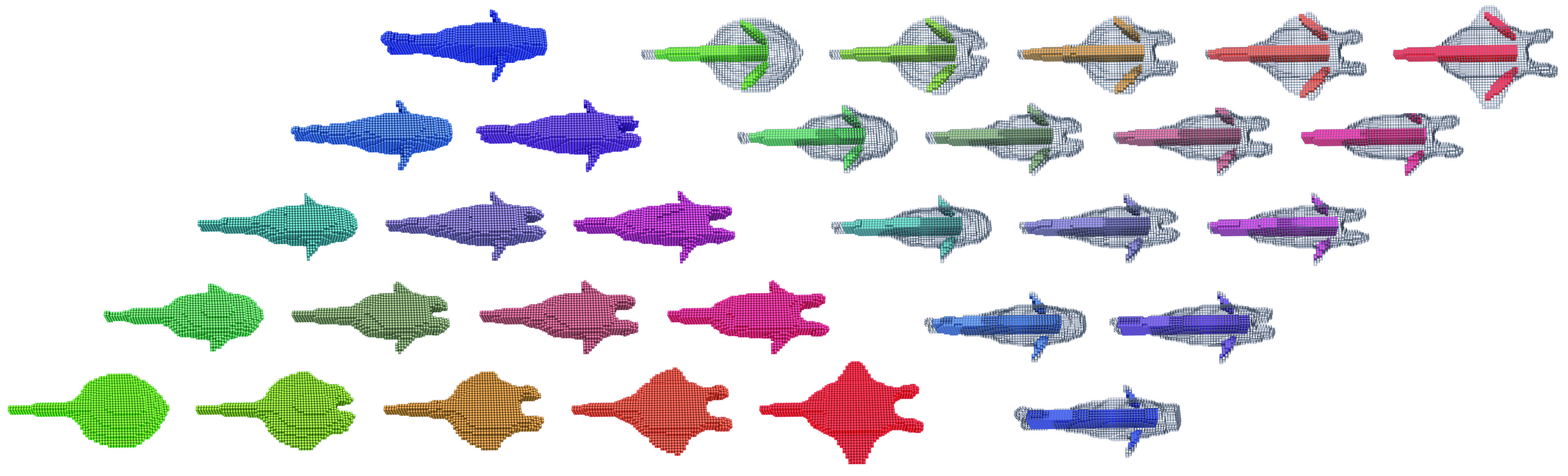
Figure 5. ”Shape exploration” experiment: Interpolation between three base shapes and their actuators. Left triangle: 12 intermediate shapes interpolated from three base shapes (red, green, and blue shapes at the corners). Right triangle: the corresponding actuator placements (colored regions) for the 12 intermediate shapes shown as wire frames, also generated by interpolating actuators in the three base shapes at the corners.

We evaluate our method’s performance with six experiments, covering shape design, co-design of geometry and control, and multi-objective design. We summarize their setup in Table 1. We run all experiments on a virtual machine instance from Google Cloud Platform with 16 Intel Xeon Scalable Processors (Cascade Lake) @ 3.1 GHz and 64 GB memory with 8 OpenMP threads in parallel.

We collect a set of meshes representing various fishes in nature as the design bases. In the pre-processing phase, we normalize and voxelize them using the same grid resolution. Grid resolutions can be found in Table 1. W use the following strategies in all our experiments to improve the numerical stability of Wasserstein barycentric interpolation: choosing basis shapes with the same topological genus, aligning their centers of mass, and running the interpolation iteration until convergence.

8.1. Design Space Exploration

Shape exploration

In this experiment, we demonstrate the capability of our shape interpolation scheme without considering optimization. In Fig. 5, we show shape and actuator interpolation between three morphologically different hand-designed base shapes from our library: a clownfish, a manta ray, and a stingray. We see from Fig. 5 that the Wasserstein barycentric interpolation is capable of generating smooth and biologically plausible intermediate shapes. Additionally, we note that our actuator interpolation generates designs adaptive to the shape’s size, as can be seen from the change of muscle size in the left and right fins.

Shape optimization

In this experiment, we demonstrate the power of our shape interpolation scheme when used in tandem with our differentiable simulator for optimizing shape design and actuator placement. We choose a shark with a tall tail and an orca with a flat tail as the base shapes. The control input is a prespecified open-loop sine wave leading to oscillatory motions on the horizontal plane (spanned by the $x$- and $y$-axes in our coordinate system), which is ill-suited for the orca but natural for the shark. We initialize the open-loop controller with $a=1$, $\omega=\frac{\pi}{6h}$, and $\varphi=0$. The objective is to find a geometric design that traverses the longest forward distance in a fixed time period $Nh$, where $N$ is the number of time steps and $h$ the time interval. We purposefully choose the shark and orca bases since we know a priori that the shark will outperform the orca in this task with the prespecified controller. Therefore, this experiment also serves as a smell test for our pipeline. Formally, the loss function is defined as

(23) $$L= -\frac{1}{|Sp|}\sum_{j\in Spine}(\bm{q}_{N,j})_{x}-(\bm{q}_{0,j})_{x}$$

(24) $$Spine= \{j|(\bm{q}_{0,j})_{y}=0\}$$

where $\bm{q}_{i,j}\in\mathcal{R}^{d}$ is the $j$-th node’s location at the $i$-th time step and $(\cdot)_{x}$ and $(\cdot)_{y}$ extracts its $x$ and $y$ coordinate, respectively. The objective encourages faster swimming speed along the desired heading direction, which is defined as the $x$-axis in all our experiments. We estimate the swimmer’s $x$-offset by averaging the $x$-offsets between the first and last time step from nodes near the spine of the swimmer, which is formally defined by a $Spine$ set consisting of nodes whose $y$ coordinate (the lateral offset) is zero when undeformed.

Fig. 6 summarizes our results in this experiment. We run our optimization algorithm with two different initial weight vectors $\bm{\alpha}$: $\bm{\alpha}=(0,1)$ which puts all weights in the orca (Fig. 6 top) and $\bm{\alpha}=(0.5,0.5)$ (Fig. 6 middle). As the control signal is known to be ill-suited for the orca, we expect the orca to have a poor performance, as is correctly reflected in the top row of Fig. 6. The optimized results from both starting shapes align with our expectation of the shark as the optimal shape for this task (Fig. 6 bottom). Our algorithm robustly converges to the optimal solution in both cases.

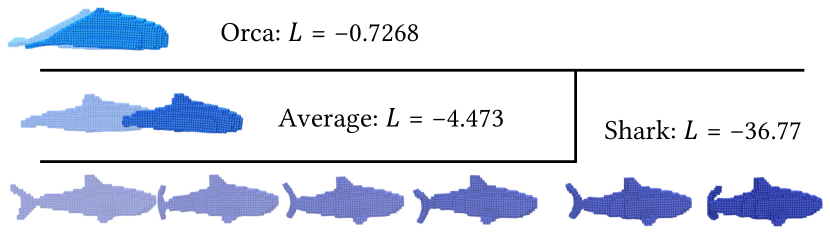
Figure 6. “Shape optimization” experiment: Performances of two initial shapes and the optimized shape. Top: the orca; Middle: the average shape between the orca and the shark; Bottom: the optimized shape found by our method, which is similar to the shark. The color on the shape indicates the weight on the two base shapes (light blue: orca, dark blue: shark). A smaller loss $L$ indicates a longer traveling distance within the same duration and is preferred in this experiment.

8.2. Co-Design of Shape and Control

Open-loop co-optimization

We now present our first co-design example, illustrating the value of our method compared to other baseline methods. The case we consider is co-optimization of both the shape and controller of an eel for the same objective described in the “shape optimization” experiment. The base shapes are two eels, i.e., slender bodies with their undulations’ wavelengths smaller than their length. One vertical eel is flag-like with a greater height than width, and the other horizontal eel is pancake-like with a greater width than height. We use the same open-loop sine wave control sequence as in the “shape optimization” experiment, except that we leave its amplitude, phase, and frequency as variables to be optimized from the initial guess with $0.5$, $0$, and $\frac{\pi}{6h}$ respectively. The decision variables for this co-optimization problem are four-dimensional, including one geometric design parameter and three control parameters. The goal is to find both an optimal shape and an optimal controller that leads to the longest distance traveled within a fixed time span. Fig. 7 shows the initial design (top row) and the optimized design (bottom row) returned by our algorithm. Since the actuation is manifested in form of a sine-wave on the horizontal plane, the optimal shape should be a vertical eel. As expected, our co-optimization algorithm correctly finds such a physical design, as well as an intensified control signal to maximize traveling distance.

For comparison, we also examine the performances of a few baseline algorithms: alt: alternating between shape and control optimization; shape-only: fixing the initial controller and optimizing the shape; control-only: fixing the initial shape and optimizing the controller; cma-es: co-optimizing both shape and controller with CMA-ES (Hansen et al., 2003), a gradient-free evolutionary algorithm. By comparing the loss-iteration curves from all of these methods (Fig. 8), we reach the following conclusions: First, co-optimizing both the shape and controller (ours, alt, and cma-es) reaches a much lower loss than only optimizing shape or control (shape-only and control-only), which is as expected. Second, gradient-based co-optimization (ours and alt) converges significantly faster than the gradient-free baseline cma-es, demonstrating the value of gradients in design optimization. Lastly, we find that simultaneously optimizing both shape and controller (ours) converges to similar results but faster than the alternating strategy alt. This observation highlights the value of our differentiable geometric design space, which makes simultaneously co-optimizing shape and control with a gradient-based algorithm possible.

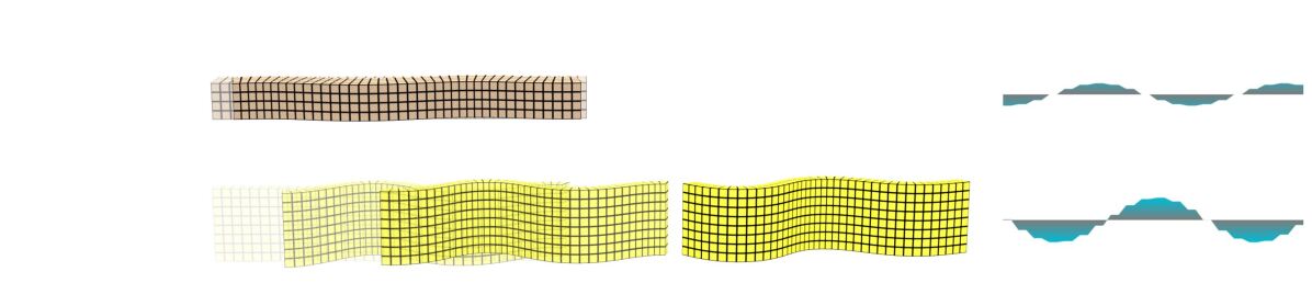
Shape                                                                         Control

Init guess

Optimized

Figure 7. “Open-loop co-optimization” experiment: The initial guess (top) and the optimized design (bottom) of the shape and control. The shapes are simulated to swim forward with the parameterized sinusoidal controller (right) from its initial position (transparent) to the final location (solid) within a fixed time period.

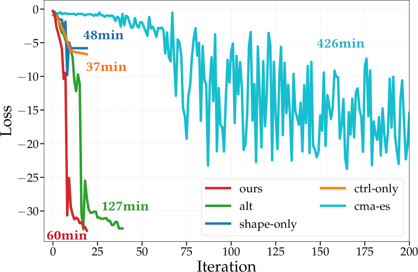
Figure 8. The loss-iteration curves for our method and four baseline algorithms evaluated in the “open-loop co-optimization” experiment. Lower losses are better. The CMA-ES loss continually oscillates and does not reach a loss lower than our method before exhausting its computational budget (250 iterations, not shown in the figure). We label the total time cost for each method with its corresponding color.

Closed-loop co-optimization

In this experiment, we replace the open-loop controller from the last experiment with a closed-loop neural network controller. We also use the three base shapes in the “shape exploration” experiment (Fig. 5) for shape interpolation. The objective is the same as in the previous experiment.

Fig. 9 and Fig. 10 show the optimal shape and controller from our method. We observe that the optimal shape assigns more weight to the clownfish and the stingray than the manta ray, likely the clownfish has a larger tail. For the controller, we also notice that the optimal neural network controller discovers a strongly oscillating pattern for the tail (Fig. 10), which aligns with our expectation for a fast swimmer. We point out that the source of periodicity in the control signal is from the temporal encoding technique: As shown in Fig. 10, learning a periodic control output becomes much more difficult when temporal encoding is disabled, leading to much worse performance (Fig. 11).

To show the value of co-optimizing both shape and control in this experiment (rather than just control), we test fixing the shape design to the three bases and optimizing the controller only. We present the loss-iteration curves for these methods in Fig. 11 and conclude that co-optimizing both the shape and control achieves significantly better performance.

Large dataset co-optimization

In a more realistic example of design pertinent to roboticists, we consider a position-keeping task in the face of an external disturbance from a constant water flow. We feed our shape interpolation a plethora of bases, including four shark variations, seven goldfish variations, and one submarine (Fig. 1). We again use a closed-loop controller as in the Experiment 4. The swimmer’s goal is to maintain its position and orientation in a stream of fast-flowing water moving against its head. Formally, our loss $L$ is defined as follows:

(25) $$L= L_{\text{perf}}+\gamma L_{\text{reg}}$$

(26) $$L_{\text{perf}}= \sum_{i}\|\bm{q}_{i,c}-\bm{q}_{\text{target}}\|_{1}$$

(27) $$L_{\text{reg}}=- \sum_{i}(\bm{q}_{i,h_{0}}-\bm{q}_{i,h_{1}})\cdot\bm{d}_{\text{target}}.$$

Here, the loss function consists of a performance loss $L_{\text{perf}}$ and a regularizer $L_{\text{reg}}$. We set the regularizer weight $\gamma=0.01$. The performance loss is defined as the cumulative offset of a node $\bm{q}_{i,c}\in\mathcal{R}^{d}$ at the $i$-th timestep with respect to a target location $\bm{q}_{\text{target}}=\bm{0}$. Here $c$ is the index of the central node in the aforementioned $Spine$ set. In short, the performance loss encourages the swimmer to stay at the origin within the given time period. Additionally, we introduce the regularizer loss to penalize controllers circling around $\bm{q}_{\text{target}}$. Here, $h_{0}$ and $h_{1}$ are indices of two prespecified nodes from the $Spine$ set. Therefore, $\bm{q}_{i,h_{0}}-\bm{q}_{i,h_{1}}$ estimates the swimmer’s heading at the $i$-th timestep. The regularizer computes the dot product between the true heading and a target heading $\bm{d}_{\text{target}}$, which is the positive $x$ unit vector, to encourage a controller that maintains orientation along the positive $x$ direction.

We report the optimal shape and controller from our method in Fig. 1. With co-optimized shape and control, the swimmer learns to leverage an oscillating motion to counter the flow and stabilize itself. We use an average of all shape bases as the initial shape for optimization. The swimmer’s shape after optimization appears mildly different from the initial guess (Fig. 1 middle and right), but that difference has a significant impact on performance. Further, the difference between the initial and optimized control signals are quite noticeable. In particular, the optimizer learns to intensify the magnitude of the control signal to counter the flow. To justify the importance of shape optimization, we compare our method to optimizing controllers with the shape fixed as each of the 12 bases. As shown in Fig. 12, our co-optimized swimmer outperforms all 12 base swimmers by a clear margin, highlighting the necessity of co-optimizing both the geometry and the control of the swimmer.

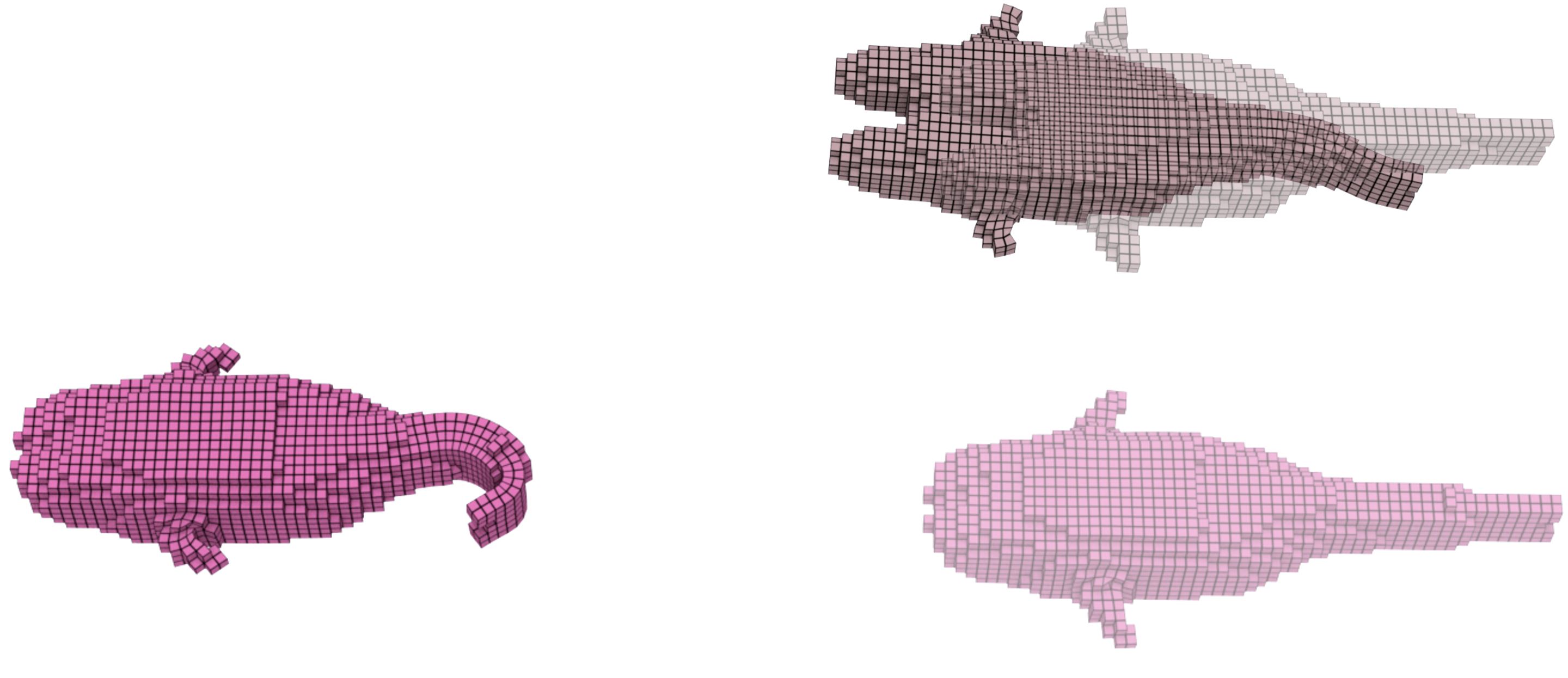
Figure 9. “Closed-loop co-optimization” experiment: Performances of the initial (top) and the optimized geometric design (bottom) of the swimmer. The color of the swimmer is interpolated with their weights $\bm{\alpha}$ from the base shapes’ colors in Fig. 5. The design is simulated to swim forward from an initial position (transparent) on the right. The swimmer’s final locations after a fixed amount of time are rendered as solid meshes. A longer traveling distance is preferred in this experiment.

Without temporal encoding                                            With temporal encoding

Fin                                      Tail                                         Fin                                      Tail

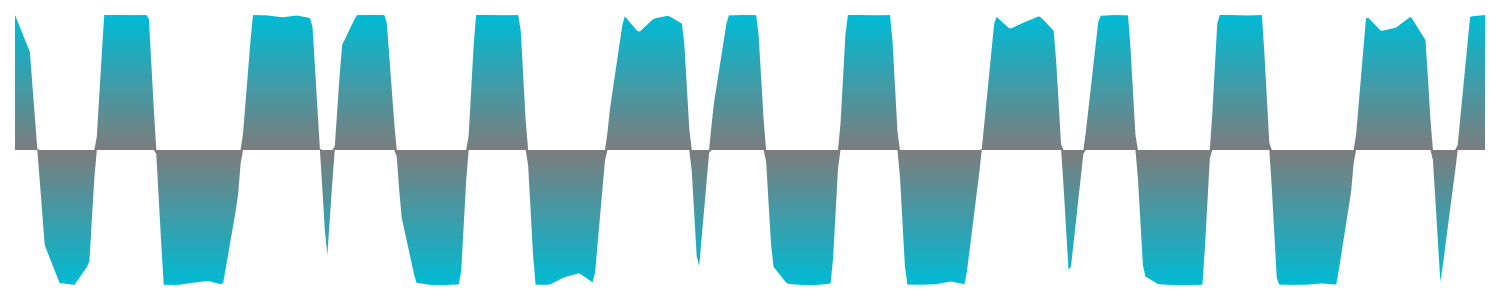
Initial guess

Optimized

Figure 10. The initial and optimized control signals generated by running our method with and without temporal encoding in the “closed-loop co-optimization” experiment.

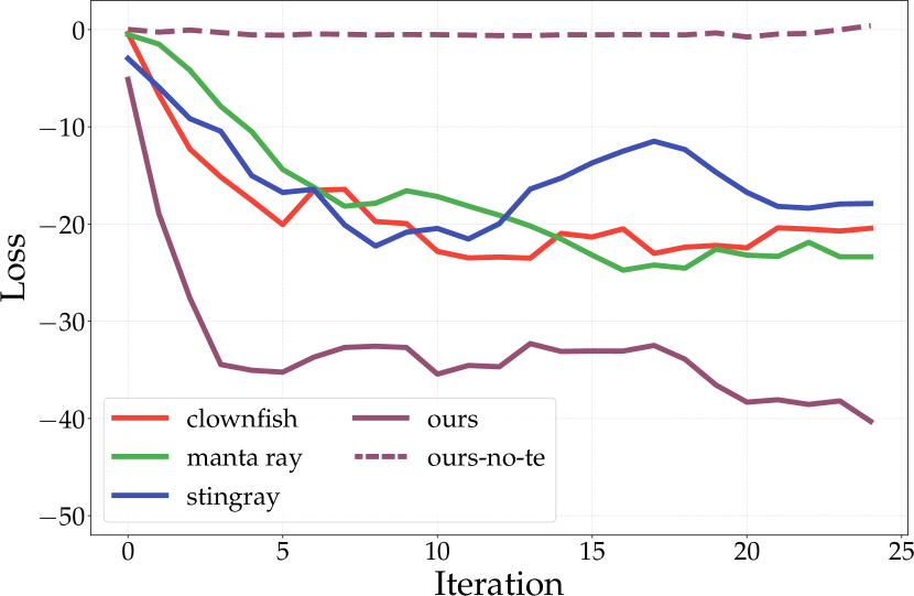
Figure 11. The loss-iteration curves for five different methods in the “closed-loop co-optimization” experiment: The curves labeled as “ours” and “ours-no-te” represent losses from our methods with and without temporal encoding. The “clownfish”, “manta ray”, and “stingray” curves record the intermediate losses from optimizing controllers with shapes fixed to the corresponding base shape. Lower losses are better.

8.3. Multi-Objective Design

Multi-objective co-optimization

Finally, we employ our method to investigate a multi-objective design problem: What is the optimal design of a swimmer for both fast and efficient forward swimming? These two objectives often conflict with each other for real marine creatures (Sfakiotakis et al., 1999); therefore, they define a gamut of designs with varying preferences on these two objectives and an interesting Pareto front.

Formally, we consider the same set of shape bases as in the “Large dataset co-optimization” experiment with two loss functions $L_{\text{speed}}$ and $L_{\text{efficiency}}$. We use the loss function in Eqn. (23) for $L_{\text{speed}}$, which reaches its minimum when the swimmer obtains the maximum average forward speed over a given time. The efficiency loss is defined as follows:

(28) $$L_{\text{efficiency}}= -\sum_{i}\frac{|P^{\text{thrust}}|}{1+|P^{\text{thrust}}|+|P^{\text{drag}}|}$$

(29) $$= -\sum_{i}\frac{|\bar{\bm{f}}_{i}^{\text{thrust}}\cdot\bar{\bm{v}}_{i}|}{1+|\bar{\bm{f}}_{i}^{\text{thrust}}\cdot\bar{\bm{v}}_{i}|+|\bar{\bm{f}}_{i}^{\text{drag}}\cdot\bar{\bm{v}}_{i}|}.$$

In short, $L_{\text{efficiency}}$ provides a measure of the energy dissipation due to the hydrodynamic drag, and minimizing $L_{\text{efficiency}}$ encourages a more efficient usage of the hydrodynamic force. We use $P_{\text{thrust}}$ and $P_{\text{drag}}$ to denote the power of hydrodynamic thrust and drag, respectively. At the $i$-th time step, we define the hydrodynamic force’s power $P^{\text{thrust}}$ as the dot product between the average hydrodynamic force $\bar{\bm{f}}_{i}^{\text{thrust}}$ on the swimmer’s surface and the average velocity $\bar{\bm{v}}_{i}$ computed from nodes in the $Spine$ set. The hydrodynamic drag’s power $P^{\text{drag}}$ is defined similarly. Finally, we add $1$ in the denominator to avoid singularities, which occurs when both the water and the swimmer are still.

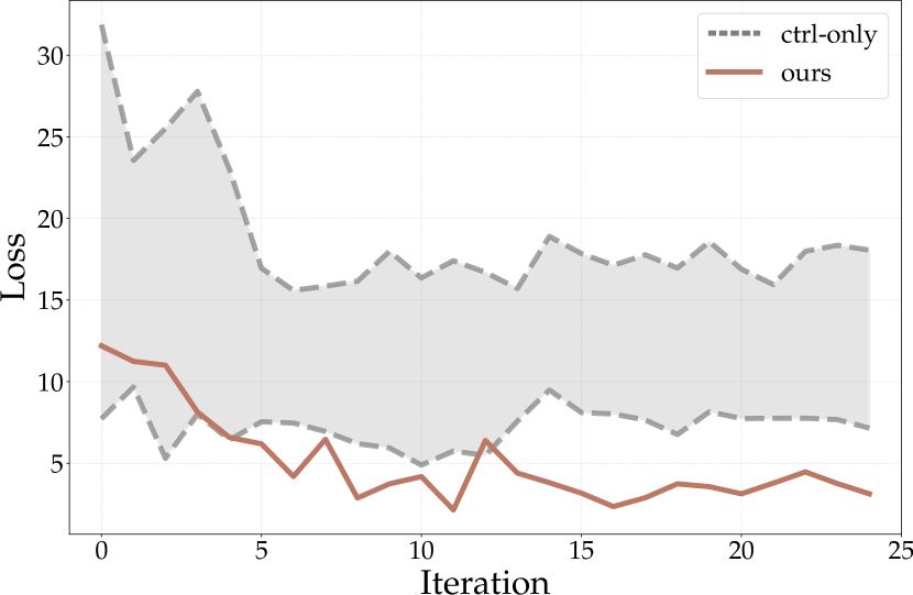
Figure 12. The loss-iteration curves for our method (ours) and optimizing control parameters with the shape fixed to each of the 12 base shapes (ctrl-only). A lower loss is better. We report the aggregate results about the 12 control-only optimizations (whose loss curves all fall in the gray area), with the lower and upper bounds of the loss curves highlighted by dashed lines.

To understand the implications of different geometry and controller designs on the two losses, we generate a gamut of swimmers and visualize their performances in the $L_{\text{speed}}$-$L_{\text{efficiency}}$ space (Fig. 13 left). Note that lower losses are better, so designs closer to the lower-left corner are preferred. To generate this gamut, we optimize the weighted sum of the two losses $w_{s}L_{\text{speed}}+w_{e}L_{\text{efficiency}}$ with $w_{s}=0,0.1,0.2,\cdots,1$ and $w_{e}=1-w_{s}$. We record all intermediate designs discovered during this process to form the gamut, with the designs on the Pareto front highlighted as white circles.

To understand the Pareto optimal designs, we sampled four swimmers along the Pareto front. Fig. 13 further shows the geometric design and neural network control outputs for the sampled swimmers. We find that the four swimmers’ shape designs are quite similar, but their controllers are significantly different. In particular, their control signals show a strong correlation with the losses: controllers preferred by faster swimmers show larger magnitudes lasting for a longer period, which exerting more powerful forces from the muscle fibers in the actuators. These sampled four swimmers, along with many others discovered in the Pareto front, form a diverse set of designs for users to choose from in case they have varying preferences.

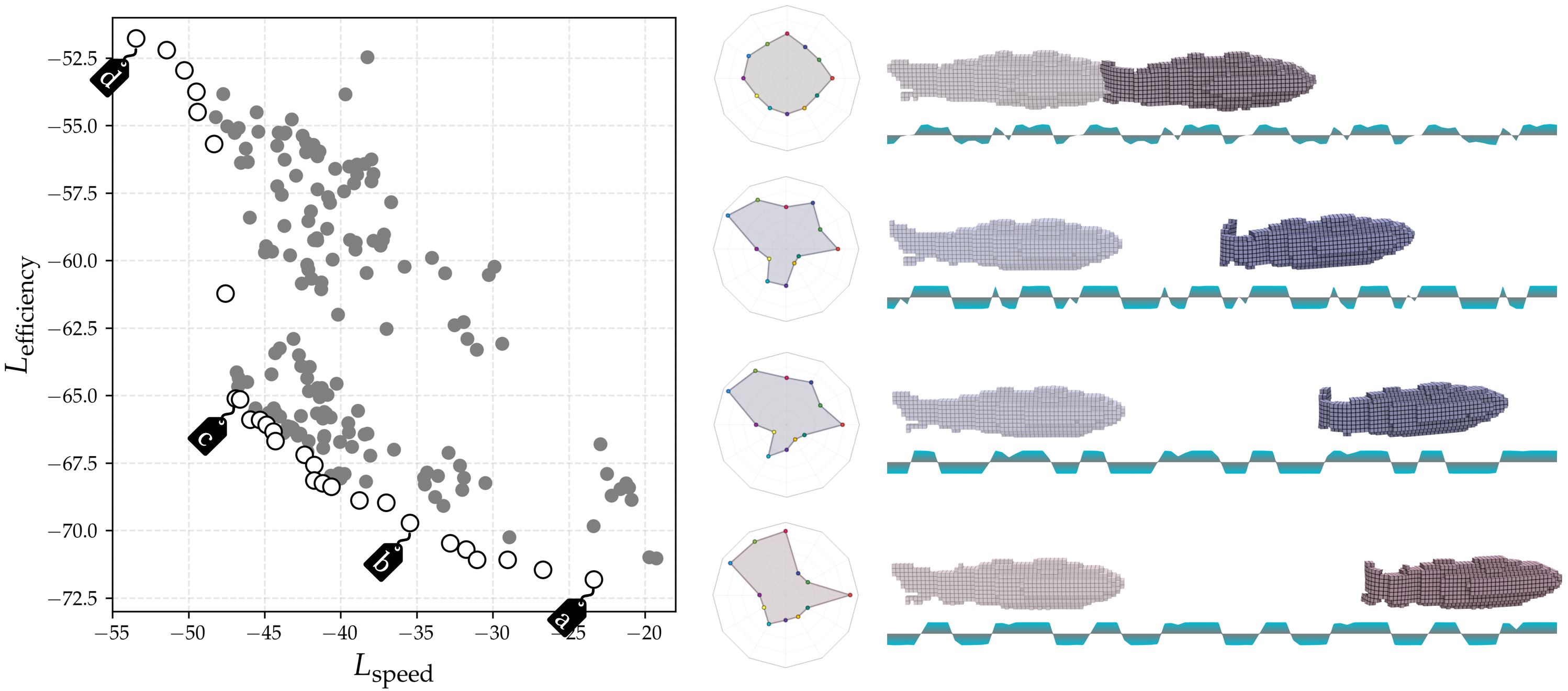
(a) high efficiency

(b) medium efficiency

(c) medium speed

(d) high speed

Figure 13. “Multi-objective co-optimization” experiment: Left: The performance gamut of the intermediate discovered designs (gray dots) and its Pareto front (white circles). Lower losses are better. Right: We show four samples, labeled as (a), (b), (c), and (d), from the Pareto front. For each sample, we show the swimmer’s initial (transparent) and final (solid) location at the beginning and end of the simulation. A larger distance between these two locations indicate a faster average speed (better $L_{speed}$). The design parameters for each sample are shown in the radar chart to its left. We plot the control signals for each sample below its initial and final locations.

8.4. Ablation Study

Gradient Scaling

The Adam optimizer we use in our experiments is a first-order gradient descent optimizer. Since such algorithms are generally not scale-invariant and we co-optimize parameters from two very different categories (geometry and control), the possible imbalance between the scale of geometry and control parameters may affect the optimizer’s performance. To examine the impact of different scales, we rerun the “closed-loop co-optimization” experiment by scaling the geometry and control parameters in three different settings: First, the default setting repeats the experiment with no changes, in which case we notice the ratio between the gradient from each geometry and control parameter is roughly 3:1. Next, in the balanced setting, we rescale the control parameters by roughly a factor of 3 so that their gradients have magnitudes comparable to those from the geometry parameters. Finally, in the reversed setting, we further rescale the control parameters until the ratio between the geometry and control gradients becomes 1:3, the reciprocal of the ratio in the default setting. We report the training curves in Fig. 14 (left), from which we notice a substantial effect from rescaling these parameters as expected. Using a scale-invariant optimizer instead of Adam could be a potential solution in the future.

Initial Guesses

To better understand the influence of different initial guesses on the performance of our method, we rerun the “large dataset co-optimization” experiment with ten randomly sampled initial shapes and controllers. Fig. 14 (right) reports the resulting ten training curves, from which we observe a consistent decrease in the loss function across all initial guesses. Still, we notice that not all random guesses converge to the same optimal solution, and some of them are trapped in different local minima. Such results are not surprising as our gradient-based method is inherently a continuous local optimization algorithm. More advanced global search algorithms might alleviate the issue of local minima, which we consider as future work.

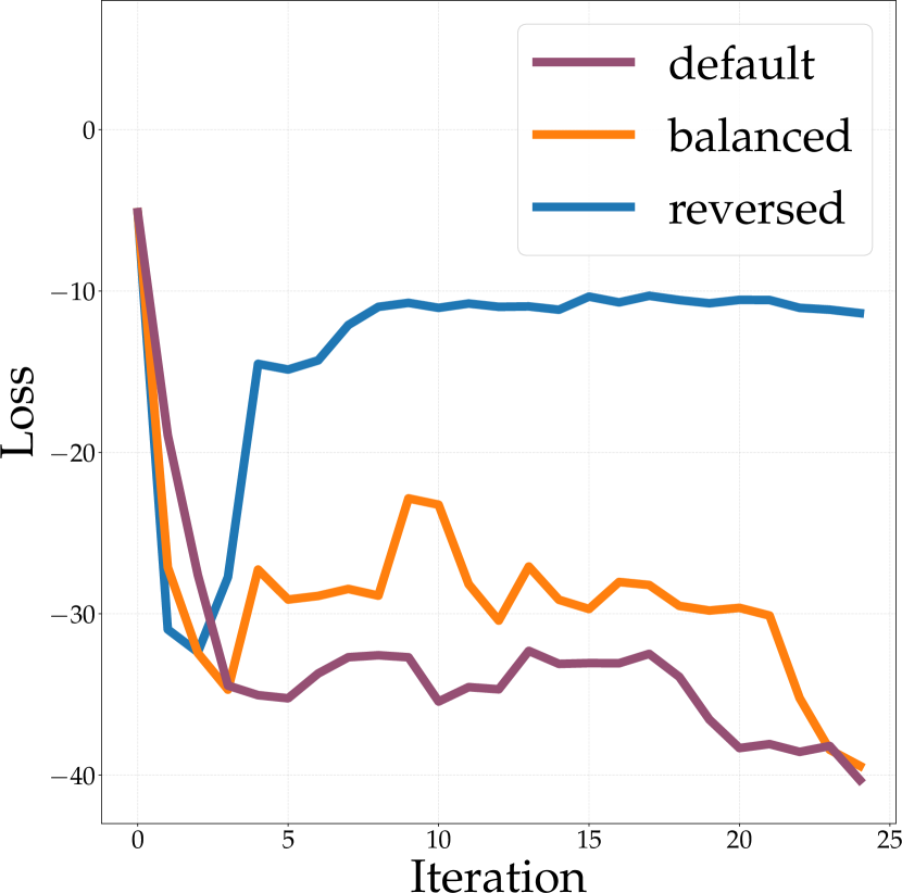
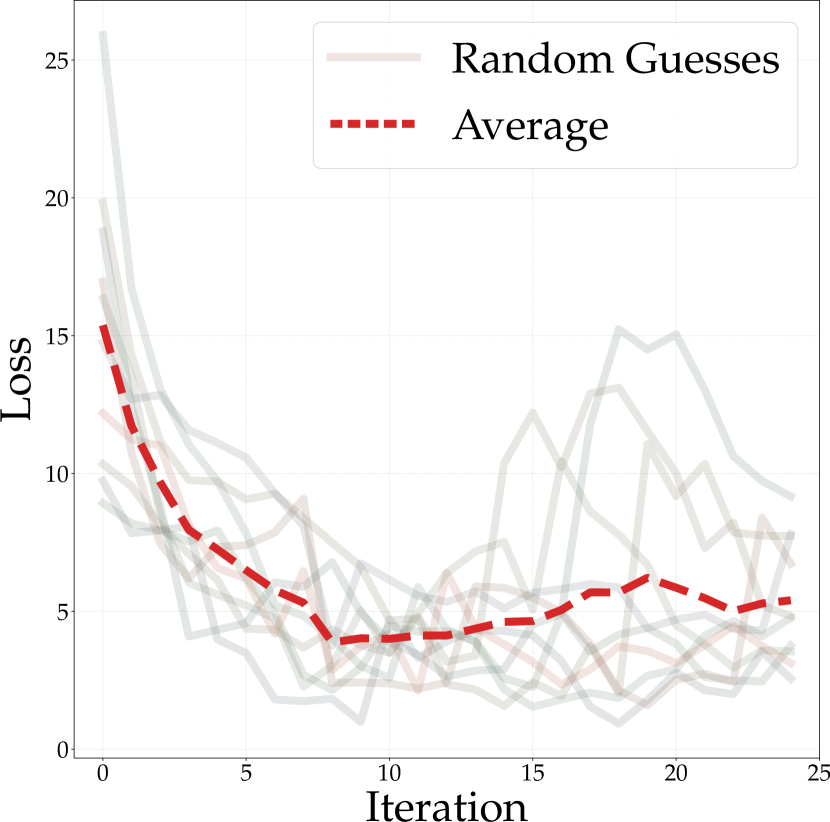
Figure 14. The loss-iteration curves for ablation studies on the “gradient scaling” experiment (left) and the “initial guesses” experiment (right) in Sec. 8.4. Lower losses are better. Left: The “default” curve reports the result without scaling the gradients. The “balanced” and “reversed” curves represent the strategies normalizing the gradients to the same average $L1$-norm and switching the scales, respectively. Right: The semitransparent curves represent the losses from different initial guesses. The red dashed line reports the average loss.

9. Conclusions, Limitations, and Future Work

We have presented a method for co-optimizing soft swimmers over control and complex geometry. By exploiting differentiable simulation and control and a basis space governed by the Wasserstein distance, we are able to generate biomimetic forms that can swim quickly, resist disturbance, or save energy. Further, we have generated designs that are Pareto-optimal in two conflicting design objectives. Our co-optimization procedure outperforms optimizing over each domain independently, demonstrating the tight interrelation of form and control in swimmer behavior.

While we have provided a first foray into the computational design of soft underwater swimmers, a number of interesting problems remain ripe for exploration. First, while our algorithm was able to interpolate between actuator shapes, those actuators were placed manually on the base shapes. A method for automating the design of muscle-based actuators for soft swimmers would be interesting. Second, our algorithm requires that the base shapes themselves be chosen by hand — it would be interesting to investigate methods for extending the morphological search beyond the Wasserstein basis space. For example, it can be combined with discrete, composition-based design methods, e.g., Zhao et al. (2020), to explore combinatorial design space. Third, certain aspects of soft swimmer design — e.g. sensing and material selection — were untouched in this work. Fourth, our simulator can be made more physically realistic by handling environmental contact as well as employing computational fluid dynamics rather than our analytical hydrodynamic model. Fifth, our work presented here investigated only virtual swimmers. It would be interesting to fabricate their physical counterparts, and research methods for overcoming the likely sim-to-real gap for physical soft swimmers. Sixth, the objectives of optimization in our experiments cover only travel distance, the ability for position maintenance, and swimming efficiency. It will be exciting to extend our algorithm to more complex goals, e.g., stability under non-constant current or controllability over a target trajectory. Finally, as our optimization scheme is a local, gradient-based method, there is no guarantee for global optimality. It would be interesting to see if our gradient-based optimization could be combined with more global heuristic searches (such as simulated annealing or evolutionary algorithms) to reap the benefits of both approaches.

- (1)
- Averkiou et al. (2014) Melinos Averkiou, Vladimir G Kim, Youyi Zheng, and Niloy J Mitra. 2014. Shapesynth: Parameterizing model collections for coupled shape exploration and synthesis. In Computer Graphics Forum, Vol. 33. Wiley Online Library, 125–134.
- Baek et al. (2015) Seung-Yeob Baek, Jeonghun Lim, and Kunwoo Lee. 2015. Isometric shape interpolation. Computers & Graphics 46 (2015), 257–263.
- Barbič et al. (2009) Jernej Barbič, Marco da Silva, and Jovan Popović. 2009. Deformable object animation using reduced optimal control. ACM Transactions on Graphics (TOG) 28, 3 (2009), 1–9.
- Barbič and Popović (2008) Jernej Barbič and Jovan Popović. 2008. Real-time control of physically based simulations using gentle forces. ACM transactions on graphics (TOG) 27, 5 (2008), 1–10.
- Belbute-Peres et al. (2018) Filipe de A Belbute-Peres, Kevin A Smith, Kelsey R Allen, Joshua B Tenenbaum, and J Zico Kolter. 2018. End-to-end differentiable physics for learning and control. In Proceedings of the 32nd International Conference on Neural Information Processing Systems. 7178–7189.
- Berlinger et al. (2018) Florian Berlinger, Mihai Duduta, Hudson Gloria, David Clarke, Radhika Nagpal, and Robert Wood. 2018. A modular dielectric elastomer actuator to drive miniature autonomous underwater vehicles. In 2018 IEEE International Conference on Robotics and Automation (ICRA). IEEE, 3429–3435.
- Bonneel et al. (2016) Nicolas Bonneel, Gabriel Peyré, and Marco Cuturi. 2016. Wasserstein barycentric coordinates: histogram regression using optimal transport. ACM Transactions on Graphics (TOG) 35, 4 (2016), 1–10.
- Bronstein et al. (2011) Alexander M Bronstein, Michael M Bronstein, Leonidas J Guibas, and Maks Ovsjanikov. 2011. Shape google: Geometric words and expressions for invariant shape retrieval. ACM Transactions on Graphics (TOG) 30, 1 (2011), 1–20.
- Chen et al. (2018) Ricky TQ Chen, Yulia Rubanova, Jesse Bettencourt, and David Duvenaud. 2018. Neural ordinary differential equations. In Proceedings of the 32nd International Conference on Neural Information Processing Systems. 6572–6583.
- Cheney et al. (2014) Nick Cheney, Robert MacCurdy, Jeff Clune, and Hod Lipson. 2014. Unshackling evolution: evolving soft robots with multiple materials and a powerful generative encoding. ACM SIGEVOlution 7, 1 (2014), 11–23.
- Corucci et al. (2016) Francesco Corucci, Nick Cheney, Hod Lipson, Cecilia Laschi, and Josh Bongard. 2016. Evolving swimming soft-bodied creatures. In ALIFE XV, The Fifteenth International Conference on the Synthesis and Simulation of Living Systems, Late Breaking Proceedings, Vol. 6.
- Degrave et al. (2019) Jonas Degrave, Michiel Hermans, Joni Dambre, and Francis wyffels. 2019. A Differentiable Physics Engine for Deep Learning in Robotics. Frontiers in Neurorobotics 13 (2019), 6.
- Della Santina et al. (2018) Cosimo Della Santina, Robert K Katzschmann, Antonio Biechi, and Daniela Rus. 2018. Dynamic control of soft robots interacting with the environment. In 2018 IEEE International Conference on Soft Robotics (RoboSoft). IEEE, 46–53.
- Du et al. (2016) Tao Du, Adriana Schulz, Bo Zhu, Bernd Bickel, and Wojciech Matusik. 2016. Computational multicopter design. ACM Transactions on Graphics (TOG) 35, 6 (2016), 1–10.
- Du et al. (2021) Tao Du, Kui Wu, Pingchuan Ma, Sebastien Wah, Andrew Spielberg, Daniela Rus, and Wojciech Matusik. 2021. DiffPD: Differentiable Projective Dynamics with Contact. arXiv preprint arXiv:2101.05917 (2021).
- Fish and Lauder (2006) FE Fish and George V Lauder. 2006. Passive and active flow control by swimming fishes and mammals. Annu. Rev. Fluid Mech. 38 (2006), 193–224.
- Fish et al. (2014) Noa Fish, Melinos Averkiou, Oliver Van Kaick, Olga Sorkine-Hornung, Daniel Cohen-Or, and Niloy J Mitra. 2014. Meta-representation of shape families. ACM Transactions on Graphics (TOG) 33, 4 (2014), 1–11.
- Geijtenbeek et al. (2013) Thomas Geijtenbeek, Michiel Van De Panne, and A Frank Van Der Stappen. 2013. Flexible muscle-based locomotion for bipedal creatures. ACM Transactions on Graphics (TOG) 32, 6 (2013), 1–11.
- Geilinger et al. (2020) Moritz Geilinger, David Hahn, Jonas Zehnder, Moritz Bächer, Bernhard Thomaszewski, and Stelian Coros. 2020. ADD: analytically differentiable dynamics for multi-body systems with frictional contact. ACM Transactions on Graphics (TOG) 39, 6 (2020), 1–15.
- Giftthaler et al. (2017) Markus Giftthaler, Michael Neunert, Markus Stäuble, Marco Frigerio, Claudio Semini, and Jonas Buchli. 2017. Automatic differentiation of rigid body dynamics for optimal control and estimation. Advanced Robotics 31, 22 (2017), 1225–1237.
- Grzeszczuk and Terzopoulos (1995) Radek Grzeszczuk and Demetri Terzopoulos. 1995. Automated learning of muscle-actuated locomotion through control abstraction. In Proceedings of the 22nd annual conference on Computer graphics and interactive techniques. 63–70.
- Ha (2019) David Ha. 2019. Reinforcement learning for improving agent design. Artificial life 25, 4 (2019), 352–365.
- Ha et al. (2018) Sehoon Ha, Stelian Coros, Alexander Alspach, James M Bern, Joohyung Kim, and Katsu Yamane. 2018. Computational design of robotic devices from high-level motion specifications. IEEE Transactions on Robotics 34, 5 (2018), 1240–1251.
- Ha et al. (2017) Sehoon Ha, Stelian Coros, Alexander Alspach, Joohyung Kim, and Katsu Yamane. 2017. Joint Optimization of Robot Design and Motion Parameters using the Implicit Function Theorem.. In Robotics: Science and systems, Vol. 8.
- Hahn et al. (2019) David Hahn, Pol Banzet, James M Bern, and Stelian Coros. 2019. Real2sim: Visco-elastic parameter estimation from dynamic motion. ACM Transactions on Graphics (TOG) 38, 6 (2019), 1–13.
- Hansen et al. (2003) Nikolaus Hansen, Sibylle D Müller, and Petros Koumoutsakos. 2003. Reducing the time complexity of the derandomized evolution strategy with covariance matrix adaptation (CMA-ES). Evolutionary computation 11, 1 (2003), 1–18.
- Hecker et al. (2008) Chris Hecker, Bernd Raabe, Ryan W Enslow, John DeWeese, Jordan Maynard, and Kees van Prooijen. 2008. Real-time motion retargeting to highly varied user-created morphologies. ACM Transactions on Graphics (TOG) 27, 3 (2008), 1–11.
- Holl et al. (2020) Philipp Holl, Nils Thuerey, and Vladlen Koltun. 2020. Learning to Control PDEs with Differentiable Physics. In International Conference on Learning Representations.
- Hu et al. (2020) Yuanming Hu, Luke Anderson, Tzu-Mao Li, Qi Sun, Nathan Carr, Jonathan Ragan-Kelley, and Frédo Durand. 2020. DiffTaichi: Differentiable Programming for Physical Simulation. International Conference on Learning Representations (2020).
- Hu et al. (2019) Yuanming Hu, Jiancheng Liu, Andrew Spielberg, Joshua B Tenenbaum, William T Freeman, Jiajun Wu, Daniela Rus, and Wojciech Matusik. 2019. ChainQueen: A real-time differentiable physical simulator for soft robotics. In 2019 International conference on robotics and automation (ICRA). IEEE, 6265–6271.
- Huang et al. (2021) Zhiao Huang, Yuanming Hu, Tao Du, Siyuan Zhou, Hao Su, Joshua B. Tenenbaum, and Chuang Gan. 2021. PlasticineLab: A Soft-Body Manipulation Benchmark with Differentiable Physics. In International Conference on Learning Representations.
- Katzschmann et al. (2019a) Robert K Katzschmann, Cosimo Della Santina, Yasunori Toshimitsu, Antonio Bicchi, and Daniela Rus. 2019a. Dynamic motion control of multi-segment soft robots using piecewise constant curvature matched with an augmented rigid body model. In 2019 2nd IEEE International Conference on Soft Robotics (RoboSoft). IEEE, 454–461.
- Katzschmann et al. (2018) Robert K Katzschmann, Joseph DelPreto, Robert MacCurdy, and Daniela Rus. 2018. Exploration of underwater life with an acoustically controlled soft robotic fish. Science Robotics 3, 16 (2018).
- Katzschmann et al. (2019b) Robert K Katzschmann, Maxime Thieffry, Olivier Goury, Alexandre Kruszewski, Thierry-Marie Guerra, Christian Duriez, and Daniela Rus. 2019b. Dynamically closed-loop controlled soft robotic arm using a reduced order finite element model with state observer. In 2019 2nd IEEE International Conference on Soft Robotics (RoboSoft). IEEE, 717–724.
- Kingma and Ba (2015) Diederik P Kingma and Jimmy Ba. 2015. Adam: A Method for Stochastic Optimization. In International Conference on Learning Representations.
- Lewis et al. (2014) John P Lewis, Ken Anjyo, Taehyun Rhee, Mengjie Zhang, Frederic H Pighin, and Zhigang Deng. 2014. Practice and Theory of Blendshape Facial Models. Eurographics (State of the Art Reports) 1, 8 (2014), 2.
- Li et al. (2019) Yunzhu Li, Jiajun Wu, Russ Tedrake, Joshua Tenenbaum, and Antonio Torralba. 2019. Learning Particle Dynamics for Manipulating Rigid Bodies, Deformable Objects, and Fluids. In International Conference on Learning Representations.
- Liang et al. (2019) Junbang Liang, Ming Lin, and Vladlen Koltun. 2019. Differentiable Cloth Simulation for Inverse Problems. In Advances in Neural Information Processing Systems. 772–781.
- Lighthill (1971) Michael James Lighthill. 1971. Large-amplitude elongated-body theory of fish locomotion. Proceedings of the Royal Society of London. Series B. Biological Sciences 179, 1055 (1971), 125–138.
- Ma et al. (2018) Pingchuan Ma, Yunsheng Tian, Zherong Pan, Bo Ren, and Dinesh Manocha. 2018. Fluid directed rigid body control using deep reinforcement learning. ACM Transactions on Graphics (TOG) 37, 4 (2018), 1–11.
- Marchese et al. (2014) Andrew D Marchese, Cagdas D Onal, and Daniela Rus. 2014. Autonomous soft robotic fish capable of escape maneuvers using fluidic elastomer actuators. Soft robotics 1, 1 (2014), 75–87.
- Marchese et al. (2016) Andrew D Marchese, Russ Tedrake, and Daniela Rus. 2016. Dynamics and trajectory optimization for a soft spatial fluidic elastomer manipulator. The International Journal of Robotics Research 35, 8 (2016), 1000–1019.
- McNamara et al. (2004) Antoine McNamara, Adrien Treuille, Zoran Popović, and Jos Stam. 2004. Fluid control using the adjoint method. ACM Transactions On Graphics (TOG) 23, 3 (2004), 449–456.
- Megaro et al. (2015) Vittorio Megaro, Bernhard Thomaszewski, Maurizio Nitti, Otmar Hilliges, Markus Gross, and Stelian Coros. 2015. Interactive design of 3d-printable robotic creatures. ACM Transactions on Graphics (TOG) 34, 6 (2015), 1–9.
- Min et al. (2019) Sehee Min, Jungdam Won, Seunghwan Lee, Jungnam Park, and Jehee Lee. 2019. SoftCon: simulation and control of soft-bodied animals with biomimetic actuators. ACM Transactions on Graphics (TOG) 38, 6 (2019), 1–12.
- Mo et al. (2019) Kaichun Mo, Paul Guerrero, Li Yi, Hao Su, Peter Wonka, Niloy J Mitra, and Leonidas J Guibas. 2019. StructureNet: hierarchical graph networks for 3D shape generation. ACM Transactions on Graphics (TOG) 38, 6 (2019), 1–19.
- Ovsjanikov et al. (2012) Maks Ovsjanikov, Mirela Ben-Chen, Justin Solomon, Adrian Butscher, and Leonidas Guibas. 2012. Functional maps: a flexible representation of maps between shapes. ACM Transactions on Graphics (TOG) 31, 4 (2012), 1–11.
- Park et al. (2019) Jeong Joon Park, Peter Florence, Julian Straub, Richard Newcombe, and Steven Lovegrove. 2019. Deepsdf: Learning continuous signed distance functions for shape representation. In Proceedings of the IEEE/CVF Conference on Computer Vision and Pattern Recognition. 165–174.
- Paszke et al. (2019) Adam Paszke, Sam Gross, Francisco Massa, Adam Lerer, James Bradbury, Gregory Chanan, Trevor Killeen, Zeming Lin, Natalia Gimelshein, Luca Antiga, et al. 2019. PyTorch: An Imperative Style, High-Performance Deep Learning Library. Advances in Neural Information Processing Systems 32 (2019), 8026–8037.
- Pathak et al. (2019) Deepak Pathak, Christopher Lu, Trevor Darrell, Phillip Isola, and Alexei A Efros. 2019. Learning to Control Self-Assembling Morphologies: A Study of Generalization via Modularity. Advances in Neural Information Processing Systems 32 (2019), 2295–2305.
- Popović et al. (2003) Jovan Popović, Steven M Seitz, and Michael Erdmann. 2003. Motion sketching for control of rigid-body simulations. ACM Transactions on Graphics (TOG) 22, 4 (2003), 1034–1054.
- Qiao et al. (2020) Yi-Ling Qiao, Junbang Liang, Vladlen Koltun, and Ming Lin. 2020. Scalable Differentiable Physics for Learning and Control. In International Conference on Machine Learning.
- Rubner et al. (2000) Yossi Rubner, Carlo Tomasi, and Leonidas J Guibas. 2000. The earth mover’s distance as a metric for image retrieval. International journal of computer vision 40, 2 (2000), 99–121.
- Sanchez-Gonzalez et al. (2020) Alvaro Sanchez-Gonzalez, Jonathan Godwin, Tobias Pfaff, Rex Ying, Jure Leskovec, and Peter Battaglia. 2020. Learning to Simulate Complex Physics with Graph Networks. In International Conference on Machine Learning.
- Schaff et al. (2019) Charles Schaff, David Yunis, Ayan Chakrabarti, and Matthew R Walter. 2019. Jointly learning to construct and control agents using deep reinforcement learning. In 2019 International Conference on Robotics and Automation (ICRA). IEEE, 9798–9805.
- Schenck and Fox (2018) Connor Schenck and Dieter Fox. 2018. SPNets: Differentiable Fluid Dynamics for Deep Neural Networks. Conference on Robot Learning (CoRL) (2018).
- Schlick (1994) Christophe Schlick. 1994. Fast Alternatives to Perlin’s Bias and Gain Functions. Graphics Gems 4 (1994), 401–404.
- Schulz et al. (2017a) Adriana Schulz, Ariel Shamir, Ilya Baran, David IW Levin, Pitchaya Sitthi-Amorn, and Wojciech Matusik. 2017a. Retrieval on parametric shape collections. ACM Transactions on Graphics (TOG) 36, 1 (2017), 1–14.
- Schulz et al. (2017b) Adriana Schulz, Cynthia Sung, Andrew Spielberg, Wei Zhao, Robin Cheng, Eitan Grinspun, Daniela Rus, and Wojciech Matusik. 2017b. Interactive robogami: An end-to-end system for design of robots with ground locomotion. The International Journal of Robotics Research 36, 10 (2017), 1131–1147.
- Sfakiotakis et al. (1999) Michael Sfakiotakis, David M Lane, and J Bruce C Davies. 1999. Review of fish swimming modes for aquatic locomotion. IEEE Journal of oceanic engineering 24, 2 (1999), 237–252.
- Sims (1994) Karl Sims. 1994. Evolving virtual creatures. In Proceedings of the 21st annual conference on Computer graphics and interactive techniques. 15–22.
- Solomon et al. (2015) Justin Solomon, Fernando De Goes, Gabriel Peyré, Marco Cuturi, Adrian Butscher, Andy Nguyen, Tao Du, and Leonidas Guibas. 2015. Convolutional wasserstein distances: Efficient optimal transportation on geometric domains. ACM Transactions on Graphics (TOG) 34, 4 (2015), 1–11.
- Spielberg et al. (2017) Andrew Spielberg, Brandon Araki, Cynthia Sung, Russ Tedrake, and Daniela Rus. 2017. Functional co-optimization of articulated robots. In 2017 IEEE International Conference on Robotics and Automation (ICRA). IEEE, 5035–5042.
- Spielberg et al. (2019) Andrew Spielberg, Allan Zhao, Yuanming Hu, Tao Du, Wojciech Matusik, and Daniela Rus. 2019. Learning-in-the-loop optimization: End-to-end control and co-design of soft robots through learned deep latent representations. Advances in Neural Information Processing Systems 32 (2019), 8284–8294.
- Tan et al. (2011) Jie Tan, Yuting Gu, Greg Turk, and C Karen Liu. 2011. Articulated swimming creatures. ACM Transactions on Graphics (TOG) 30, 4 (2011), 1–12.
- Thieffry et al. (2018) Maxime Thieffry, Alexandre Kruszewski, Christian Duriez, and Thierry-Marie Guerra. 2018. Control Design for Soft Robots Based on Reduced-Order Model. IEEE Robotics and Automation Letters 4, 1 (2018), 25–32.
- Triantafyllou and Triantafyllou (1995) Michael S Triantafyllou and George S Triantafyllou. 1995. An efficient swimming machine. Scientific american 272, 3 (1995), 64–70.
- Van Diepen and Shea (2019) Merel Van Diepen and Kristina Shea. 2019. A spatial grammar method for the computational design synthesis of virtual soft locomotion robots. Journal of Mechanical Design 141, 10 (2019).
- Vaswani et al. (2017) Ashish Vaswani, Noam Shazeer, Niki Parmar, Jakob Uszkoreit, Llion Jones, Aidan N Gomez, Łukasz Kaiser, and Illia Polosukhin. 2017. Attention is all you need. In Proceedings of the 31st International Conference on Neural Information Processing Systems. 6000–6010.
- Wampler and Popović (2009) Kevin Wampler and Zoran Popović. 2009. Optimal gait and form for animal locomotion. ACM Transactions on Graphics (TOG) 28, 3 (2009), 1–8.
- Wang et al. (2018) Tingwu Wang, Yuhao Zhou, Sanja Fidler, and Jimmy Ba. 2018. Neural Graph Evolution: Towards Efficient Automatic Robot Design. In International Conference on Learning Representations.
- Won and Lee (2019) Jungdam Won and Jehee Lee. 2019. Learning body shape variation in physics-based characters. ACM Transactions on Graphics (TOG) 38, 6 (2019), 1–12.
- Yang et al. (2019) Guandao Yang, Xun Huang, Zekun Hao, Ming-Yu Liu, Serge Belongie, and Bharath Hariharan. 2019. Pointflow: 3d point cloud generation with continuous normalizing flows. In Proceedings of the IEEE/CVF International Conference on Computer Vision. 4541–4550.
- Zhao et al. (2020) Allan Zhao, Jie Xu, Mina Konaković-Luković, Josephine Hughes, Andrew Spielberg, Daniela Rus, and Wojciech Matusik. 2020. RoboGrammar: graph grammar for terrain-optimized robot design. ACM Transactions on Graphics (TOG) 39, 6 (2020), 1–16.