Partition-Guided GANs

Abstract

Despite the success of Generative Adversarial Networks (GANs), their training suffers from several well-known problems, including mode collapse and difficulties learning a disconnected set of manifolds. In this paper, we break down learning complex high dimensional distributions to simpler sub-tasks, supporting diverse data samples. Our solution relies on designing a partitioner that breaks the space into smaller regions, each having a simpler distribution, and training a different generator for each partition. This is done in an unsupervised manner without requiring any labels.

We formulate two desired criteria for the space partitioner that aid the training of our mixture of generators: 1) to produce connected partitions and 2) provide a proxy of distance between partitions and data samples, along with a direction for reducing that distance. These criteria are developed to avoid producing samples from places with non-existent data density, and also facilitate training by providing additional direction to the generators. We develop theoretical constraints for a space partitioner to satisfy the above criteria. Guided by our theoretical analysis, we design an effective neural architecture for the space partitioner that empirically assures these conditions. Experimental results on various standard benchmarks show that the proposed unsupervised model outperforms several recent methods.

1 Introduction

Generative adversarial networks (GANs) [20] have gained remarkable success in learning the underlying distribution of observed samples. However, their training is still unstable and challenging, especially when the data distribution of interest is multimodal. This is particularly important due to both empirical and theoretical evidence that suggests real data also conforms to such distributions [57, 72].

Improving the vanilla GAN, both in terms of training stability and generating high fidelity images, has been the subject of great interest in the machine learning literature [1, 13, 21, 47, 50, 52, 54, 61, 64, 67, 80]. One of the main problems is mode collapse, where the generator fails to capture the full diversity of the data. Another problem, which hasn’t been fully explored, is the mode connecting problem [36, 71]. As we explain in detail in Section 2, this phenomenon occurs when the GAN generates samples from parts of the space where the true data is non-existent, caused by using a continuous generator to approximate a distribution with disconnected support. Moreover, GANs are also known to be hard to train due to the unreliable gradient provided by the discriminator.

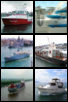
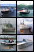
    Real             Generated

(a) Partition 13

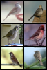
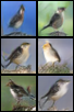
    Real             Generated

(b) Partition 47

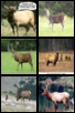
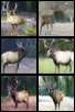
    Real             Generated

(c) Partition 69

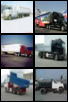
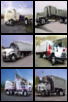
    Real             Generated

(d) Partition 85

Figure 1: Examples of unsupervised partitioning and their corresponding real/generated samples on the CIFAR-10 dataset.

Our solution to alleviate the aforementioned problems is introducing an unsupervised space partitioner and training a different generator for each partition. Figure 1 illustrates real and generated samples from several inferred partitions.

Having multiple generators, which are focused on different parts/modes of the distribution, reduces the chances of missing a mode. This also mitigates mode connecting because the mixture of generators is no longer restricted to be a continuous function responsible for generating from a data distribution with potentially disconnected manifolds. In this context, an effective space partitioner should place disconnected data manifolds in different partitions. Therefore, assuming semantically similar images are in the same connected manifold, we use contrastive learning methods to learn semantic representations of images and partition the space using these embeddings.

We show that the space partitioner can be utilized to define a distance between points in the data space and partitions. The gradient of this distance can be used to encourage each generator to focus on its corresponding region by providing a direction to guide it there. In other words, by penalizing a generator when its samples are far from its partition, the space partitioner can guide the generator to its designated region. Our partitioner’s guide is particularly useful where the discriminator does not provide a reliable gradient, as it can steer the generator in the right direction.

However, for a reliable guide, the distance function must follow certain characteristics, which are challenging to achieve. For example, to avoid misleading the GANs’ training, the distance should have no local optima outside the partition. In Section 4.2, we formulate sufficient theoretical conditions for a desirable metric and attain them by enforcing constraints on the architecture of the space partitioner. This also guarantees connected partitions in the data space, which further mitigates mode connecting as a by-product.

We perform comprehensive experiments on StackedMNIST [45, 46, 70], CIFAR-10 [39], STL-10 [12] and ImageNet [63] without revealing the class labels to our model. We show that our method, Partition-Guided Mixture of GAN (PGMGAN), successfully recovers all the modes and achieves higher Inception Score (IS) [67] and Frechet Inception Distance (FID) [26] than a wide range of supervised and unsupervised methods.

Our contributions can be summarized as:

• Providing a theoretical lower bound on the total variational distance of the true and estimated densities using a single generator.

• Introducing a novel differentiable space partitioner and demonstrating that simply training a mixture of generators on its partitions alleviates mode collapse/connecting.

• Providing a practical way (with theoretical guarantees) to guide each generator to produce samples from its designated region, further improving mode collapse/connecting. Our experiments show significant improvement over relevant baselines in terms of FID and IS, confirming the efficacy of our model.

• Elaborating on the design of our loss and architecture by making connection to supervised GANs that employ a classifier. We explain how PGMGAN avoids their shortcomings.

2 Mode connecting problem

Suppose the data distribution is supported on a set of disconnected manifolds embedded within a higher-dimensional space. Since continuous functions preserve the space connectivity [35], one can never expect to have an exact approximation of this distribution by applying a continuous function ($G_{{\bm{\theta}}}$) to a random variable with a connected support. Furthermore, if we restrict $G_{{\bm{\theta}}}$ to the class of c-Lipschitz functions, the distance between the true density and approximated will always remain more than a certain positive value. In fact, the generator would either have to discard some of the data manifolds or connect the manifolds. The former can be considered a form of mode collapse, and we refer to the latter as the mode connecting problem.

The following theorem formally describes the above statement and provides a lower bound for the total variation distance between the true and estimated densities.

Theorem 1.

Let $p_{\rm{data}}$ be a distribution supported on a set of disjoint manifolds $\mathcal{M}_{1},\dots,\mathcal{M}_{k}$ in ${\mathbb{R}}^{d}$, and $[\pi_{1},\dots,\pi_{k}]$ be the probabilities of being from each manifold. Let $G_{{\bm{\theta}}}$ be a c-Lipschitz function, and $p_{\rm{model}}$ be the distribution of $G_{{\bm{\theta}}}({\mathbf{z}})$, where ${\mathbf{z}}\sim\mathcal{N}(0,{\bm{I}}_{n})$, then:

$$d_{TV}(p_{\rm{data}},p_{\rm{model}})\geq\sum|\pi_{i}-p_{i}|\geq\delta$$

where $d_{TV}$ is the total variation distance and:

$$\pi_{i}^{*} :=\min(\pi_{i},1-\pi_{i})$$

$$p_{i} :=p_{\rm{model}}(\mathcal{M}_{i})$$

$$\delta\, :=\max_{i}{\{\pi_{i}^{*}-\Phi(\Phi^{-1}(\pi_{i}^{*})-d_{i}/c)\}}$$

$$d_{i} :=\inf\{||{\bm{x}}-{\bm{y}}||~{}~{}|~{}{\bm{x}}\in\mathcal{M}_{i},{\bm{y}}\in\mathcal{M}_{j},j\neq i\}$$

$d_{i}$ is the distance of manifold $\mathcal{M}_{i}$ from the rest, and $\Phi$ is the CDF of the univariate standard normal distribution. Note $\delta$ is strictly larger than zero iff $\exists i:\,d_{i},\pi_{i}^{*}\neq 0$.

According to Theorem 1, the distance between the estimated density and the data distribution can not converge to zero when $G_{{\bm{\theta}}}$ is a Lipschitz function. It is worth noting that this assumption holds in practice for most neural architectures as they are a composition of simple Lipschitz functions. Furthermore, most of the state-of-the-art GAN architectures (e.g., BigGAN [5] or SAGAN [82]) use spectral normalization in their generator to stabilize their training, which promotes Lipschitzness.

3 Related work

Apart from their application in computer vision [28, 29, 30, 31, 33, 78, 83, 86], GANs have also been been employed in natural language processing [43, 44, 81], medicine [68, 37] and several other fields [16, 51, 60]. Many of recent research have accordingly focused on providing ways to avoid the problems discussed in Section 2 [45, 53].

Mode collapse For instance, Metz et al. [53] unroll the optimization of the discriminator to obtain a better estimate of the optimal discriminator at each step, which remedies mode collapse. However, due to high computational complexity, it is not scalable to large datasets. VEEGAN [70] adds a reconstruction term to bi-directional GANs [15, 14] objective, which does not depend on the discriminator. This term can provide a training signal to the generator even when the discriminator does not. PacGAN [45] changes the discriminator to make decisions based on a pack of samples. This change mitigates mode collapse by making it easier for the discriminator to detect lack of diversity and naturally penalize the generator when mode collapse happens. Lucic et al. [49], motivated by the better performance of supervised-GANs, propose using a small set of labels and a semi-supervised method to infer the labels for the entire data. They further improve the performance by utilizing an auxiliary rotation loss similar to that of RotNet [17].

Mode connecting Based on Theorem 1, to avoid mode connecting one has to either use a latent variable ${\mathbf{z}}$ with a disconnected support, or allow $G_{{\bm{\theta}}}$ to be a discontinuous function [27, 36, 40, 46, 65].

To obtain a disconnected latent space, DeLiGAN [22] samples ${\mathbf{z}}$ from a mixture of Gaussian, while Odena et al. [59] add a discreet dimension to the latent variable. Other methods dissect the latent space post-training using some variant of rejection sampling, for example, Azadi et al. [2] perform rejection sampling based on the discriminator’s score, and Tanielian et al. [71] reject the samples where the generator’s Jacobian is higher than a certain threshold.

The discontinuous generator method is mostly achieved by learning multiple generators, with the primary motivation being to remedy mode-collapse, which also reduces mode connecting. Both MGAN [27] and DMWGAN [36] employ $K$ different generators while penalizing them from overlapping with each other. However, these works do not explicitly address the issue when some of the data modes are not being captured. Also, as shown in Liu et al. [46], MGAN is quite sensitive to the choice of $K$. By contrast, Self-Conditioned GAN [46] clusters the space using the discriminator’s final layer and uses the labels as self-supervised conditions. However, in practice, their clustering does not seem to be reliable (e.g., in terms of NMI for labeled datasets), and the features highly depend on the choice of the discriminator’s architecture. In addition, there is no guarantee that the generators will be guided to generate from their assigned clusters. GAN-Tree [40] uses hierarchical clustering to address continuous multi-modal data, with the number of parameters increasing linearly with the number of clusters. Thus it is limited to very few cluster numbers (e.g., 5) and can only capture a few modes.

Another recently expanding direction explores the benefit of using image augmentation techniques for generative modeling. Some works simply augment the data using various perturbations (e.g., random crop, horizontal flipping) [34]. Others [9, 49, 85] incorporated regularization on top of the augmentations, for example CRGAN [84] enforces consistency for different image perturbations. ADA [32] processes each image using non-leaking augmentations and adaptively tunes the augmentation strength while training. These works are orthogonal to ours and can be combined with our method.

4 Method

This section first describes how GANs are trained on a partitioned space using a mixture of generators/discriminators and the unified objective function required for this goal. We then explain our differentiable space partitioner and how we guide the generators towards the right region. We conclude the section by making connections to supervised GANs, which use an auxiliary classifier [56, 59].

Multi-generator/discriminator objective: Given a partitioning of the space, we train a generator ($G_{i}$) and a discriminator ($D_{i}$) for each region. To avoid over-parameterization and allow information sharing across different regions, we employ parameter sharing across different $G_{i}$ ($D_{i}$) by tying their parameters except the input (last) layer. The mixture of these generators serves as our main generator $G$. We use the following objective function to train our GANs:

$$\sum_{i}^{k}\pi_{i}\left[\min_{G_{i}}\max_{D_{i}}V(D_{i},G_{i},{A}_{i})\right]$$ (1)

where ${A}_{1},{A}_{2},...,{A}_{k}$ is a partitioning of the space, $\pi_{i}:=p_{data}({\mathbf{x}}\in{A}_{i})$ and:

$$V(D,G,{A})=\, \mathbb{E}_{\bm{x}\sim p_{\text{data}}(\bm{x}|{\bm{x}}\in{A})}[\log D(\bm{x})]\,\,+$$

$$\mathbb{E}_{\bm{z}\sim p_{\bm{z}}(\bm{z}|G(\bm{z})\in{A})}[\log(1-D(G(\bm{z})))]$$ (2)

We motivate this objective by making connection to the Jensen–Shannon distance (${\rm JSD}$) between the distribution of our mixture of generators and the data distribution in the following Theorem.

Theorem 2.

Let $P=\sum_{i}^{k}\pi_{i}p_{i}$ , $Q=\sum_{i}^{k}\pi_{i}q_{i}$ , and ${A}_{1},{A}_{2},...,{A}_{K}$ be a partitioning of the space, such that the support of each distribution $p_{i}$ and $q_{i}$ is ${A}_{i}$. Then:

$${\rm JSD}(P\parallel Q)=\sum_{i}\pi_{i}{\rm JSD}(p_{i}\parallel q_{i})$$ (3)

4.1 Partition GAN

Space Partitioner: Based on Theorem 1, an ideal space partitioner should place disjoint data manifolds in different partitions to avoid mode connecting (and consequently mode collapse). It is also reasonable to assume that semantically similar data points lay on the same manifold. Hence, we train our space partitioner using semantic embeddings.

We achieve this goal in two steps: 1) Learning an unsupervised representation for each data point, which is invariant to transformations that do not change the semantic meaning. 2) Training a partitioner based on these features, where data points with similar embeddings are placed in the same partition.

Learning representations: We follow the self-supervised literature [7, 8, 24] to construct image representations.

These methods generally train the networks via maximizing the agreement between augmented views (e.g., random crop, color distortion, rotation, etc.) of the same scene, while minimizing the agreement of views from different scenes. To that end, they optimize the following contrastive loss:

$$\sum_{(i,j)\in P}\log\frac{\exp(\mathrm{sim}({\mathbf{h}}_{i},{\mathbf{h}}_{j})/\tau)}{\sum_{k=1}^{2N}\bm{1}_{k\neq i}\exp(\mathrm{sim}({\mathbf{h}}_{i},{\mathbf{h}}_{k})/\tau)}$$ (4)

where ${\mathbf{h}}$ is the embedding for image ${\mathbf{x}}$, $(i,j)$ is a positive pair (i.e., two views of the same image) and $(i,k)$ refers to negative pairs related to two different images. We refer to this network as pretext, implying the task being solved is not of real interest but is solved only for the true purpose of learning a suitable data representation.

Learning partitions: To perform the partitioning step, one can directly apply K-means on these semantic representations. However, this may result in degenerated clusters where one partition contains most of the data [6, 75]. Inspired by Van Gansbek et al. [75], to mitigate this challenge, we first make a k-nearest neighbor graph ${\mathcal{G}}=({\mathcal{V}},{\mathcal{E}})$ based on the representations ${\mathbf{h}}$ of the data points. We then train an unsupervised model that motivates connected points to reside in the same cluster and disconnected points to reside in distinct clusters. More specifically, we train a space partitioner $S:{\mathbb{R}}^{d}\to[0,1]^{k}$ to maximize:

$$\sum_{(i,j)\in{\mathcal{E}}} \log\left(S({\mathbf{x}}_{i})^{T}\cdot S({\mathbf{x}}_{j})\right)-$$

$$\alpha\sum_{i\in{\mathcal{V}}}H_{C}(S({\mathbf{x}}_{i})))+\beta H_{C}(\sum_{i\in{\mathcal{V}}}\frac{S({\mathbf{x}}_{i})}{N})$$ (5)

where $H_{C}(.)$ is the entropy function of the categorical distribution based on its probability vector. The first term in Equation 4.1 motivates the neighbors in ${\mathcal{G}}$ to have similar class probability vectors, with the $\log$ function used to significantly penalize the classifier if it assigns dissimilar probability vector to two neighboring points. The last term is designed to avoid placing all the data points in the same category by motivating the average cluster probability vector to be similar to the uniform distribution. The middle term is intended to promote the probability vector for each data point to significantly favor one class over the other. This way, we can be more confident about the cluster id of each data point. Furthermore, if the average probability of classes has a homogeneous mean (because of the last term), we can expect the number of data points in each class to not degenerate.

To train $S$ efficiently, both in term of accuracy and computational complexity, we initialize $S$ using the already trained network of unsupervised features. More specifically, for:

$${\mathbf{h}}=W_{2}^{\textit{pretext}}\sigma(W_{1}^{\textit{pretext}}\phi_{0}({\mathbf{x}}))$$

we initialize $S$ as follows:

$$S^{\textit{init}}({\mathbf{x}})=\textit{softmax}(W_{0}^{\textit{partitioner}}\phi_{0}({\mathbf{x}}))$$

where $\sigma$ is an activation function, and $W_{0}^{\textit{partitioner}}$ is a randomly initialized matrix; we ignore the bias term here for brevity. We drop the sub index $0$, from $W_{0}^{\textit{partitioner}}$ and $\phi_{0}$ to refer to their post-training versions. Given a fully trained $S$, each point ${\mathbf{x}}$ is assigned to partition $A_{i}$, based on the argmax of the probability vector of $S({\mathbf{x}})$.

4.2 Partition-Guided GAN

In this section we describe the design of guide and its properties. As stated previously, we want to guide each generator $G_{i}$ to its designated region $A_{i}$ by penalizing it the farther its current generated samples are from $A_{i}$.

A simple, yet effective proxy of measuring this distance can be attained using the already trained space partitioner. Let $f_{i}$s denote the partitioner’s last layer logits, expressed as

$$[f_{1}({\mathbf{x}}),\dots,f_{k}({\mathbf{x}})]^{T}:=W^{\textit{partitioner}}\phi({\mathbf{x}}).$$

and define the desired distance as:

$$R_{i}({\mathbf{x}}):=\sum_{c}(f_{c}({\mathbf{x}})-f_{i}({\mathbf{x}}))_{+}$$ (6)

Property $1$. It is easy to show that for any generated sample ${\mathbf{x}}$, $R_{i}({\mathbf{x}})$ achieves a larger value, the less likely $S$ believes ${\mathbf{x}}$ to be from partition $A_{i}$. This is clear from how we defined $R_{i}$, the more probability mass $S({\mathbf{x}})$ assigns any class $c\neq i$, the larger the value of $R_{i}({\mathbf{x}})$.

Property $2$. It is also straightforward to see that $R_{i}({\mathbf{x}})$ is always non-negative and obtains its minimum (zero) only on the $A_{i}$^th partition:

$$\begin{split}{\mathbf{x}}\in{A}_{i}\iff&f_{i}({\mathbf{x}})\geq f_{c}({\mathbf{x}});\quad\forall c\in[1:k]\\ \iff&R_{i}({\mathbf{x}})=\sum_{c}(f_{c}({\mathbf{x}})-f_{i}({\mathbf{x}}))_{+}=0\end{split}$$ (7)

Therefore, we guide each generator $G_{i}$ to produce samples from its region by adding a penalization term to its canonical objective function:

$$\min_{G_{i}}\sum_{j=1}^{n}\log(1-D_{i} (G_{i}(\bm{z}^{(j)}))))$$

$$+\lambda \sum_{j}R_{i}(G_{i}(\bm{z}^{(j)}))/n.$$ (8)

Intuitionally, $G_{i}$ needs to move its samples towards partition $A_{i}$ in order to minimize the newly added term. Fortunately, given the differentiability of $R_{i}(.)$ with respect to its inputs and Property $1$, $R_{i}$ can provide the direction for $G_{i}$ to achieve that goal.

It is also worth noting that $R_{i}$ should not interfere with the generator/discriminator as long as $G_{i}$’s samples are within ${A}_{i}$. Otherwise, this may lead to the second term favoring parts of ${A}_{i}$ over others and conflicting with the discriminator. Property $2$ assures that learning the distribution of $p_{data}$ over ${A}_{i}$ remains the responsibility of $D_{i}$. We also use this metric to ensure each trained generator $G_{i}$ only draws samples from within its region by only accepting samples with $R_{i}({\mathbf{x}})$ being equal to zero.

A critical point left to consider is the possibility of $G_{i}$ getting fooled to generate samples from outside ${A}_{i}$, by falling in local optima of $R_{i}({\mathbf{x}})$. In the remaining part of this section, we will explain how the architecture design of the space partitioner $S$ avoids this issue. In addition, it will also guarantee the norm of the gradient provided by $R_{i}$ to always be above a certain threshold.

Avoiding local optima: We can easily obtain a guide $R_{i}$ with no local optima, if achieving a good performance for the partitioner was not important. For instance, a simple single-linear-layer neural network as $S$ would do the trick. The main challenge comes from the fact that we need to perform well on partitioning , which usually requires deep neural networks while avoiding local optima. We fulfill this goal by first finding a sufficient condition to have no local optima and then trying to enforce that condition by modifying the ResNet [25] architecture.

The following theorem states the sufficient condition:

Theorem 3.

Let $\phi({\mathbf{x}}):{\mathbb{R}}^{d}\to{\mathbb{R}}^{d}$ be a $C^{1}$ (differentiable with continuous derivative) function, $W^{\textit{partitioner}}\in{\mathbb{R}}^{k\times d}$, and $R_{i}$ as defined in Eq 6. If there exists $c_{0}>0$, such that:

$$\forall\,{\mathbf{x}},{\mathbf{y}}\in{\mathbb{R}}^{d},~{}~{}~{}~{}c_{0}||{\mathbf{x}}-{\mathbf{y}}||\leq||\phi({\mathbf{x}})-\phi({\mathbf{y}})||,$$

then for every $i\in[1:k]$, every local optima of $R_{i}$ is a global optima, and there exists a positive constant $b_{0}>0$ such that:

$$\forall{\mathbf{x}}\in{\mathbb{R}}^{d}\setminus A_{i},~{}~{}~{}~{}b_{0}\leq||\nabla R_{i}({\mathbf{x}})||$$

where $A_{i}=\{{\mathbf{x}}|{\mathbf{x}}\in{\mathbb{R}}^{d},R_{i}({\mathbf{x}})=0\}$. Furthermore $A_{i}$ is a connected set for all $i$’s.

The proof is provided in the Appendix. Next we describe how to satisfy this constraint in practice.

Motivated by the work of Behrmann et al. [3] who design an invertible network without significantly sacrificing their classification accuracy, we implement $\phi$ by stacking several residual blocks, $\phi({\mathbf{x}})=B_{T}\circ B_{T-1}\circ\cdots\circ B_{1}({\mathbf{x}})$, where:

$$B_{t+1}({\mathbf{x}}^{(t)})={\mathbf{x}}^{(t+1)}:={\mathbf{x}}^{(t)}+\psi_{t}({\mathbf{x}}^{(t)})$$

and ${\mathbf{x}}^{(t)}$ refers to the out of the $t$^th residual block. Figure 2, gives an overview of the proposed architecture.

We model each $\psi_{t}$ as a series of $m$ convolutional layers, each having spectral norm $L<1$ intertwined by $1$-Lipschitz activation functions (e.g., ELU, ReLU, LeakyReLU). Thus it can be easily shown for all ${\mathbf{x}}^{(t)},{\mathbf{y}}^{(t)}\in{\mathbb{R}}^{d}$:

$$(1-L^{m})||{\mathbf{x}}^{(t)}-{\mathbf{y}}^{(t)}||\leq||B_{t}({\mathbf{x}}^{(t)})-B_{t}({\mathbf{y}}^{(t)})||.$$

This immediately results in the condition required in Theorem 3 by letting $c_{0}:=(1-L^{m})$.

Figure 2: Diagram of proposed partitioner and guide. We employ spectral normalization for each convolutional layer to make each layer (as a function) have Lipschitz constant of less than one. The details of our architecture is provided in the Appendix.

4.3 Connection to supervised GANs

In this section, we make a connection between our unsupervised GAN and some important work in the supervised regime. This will help provide better insight into why the mentioned properties of guide are important. Auxiliary Classifier GAN [59] has been one of the well-known supervised GAN methods which uses the following objective function:

$$\underset{{G,C}}{\min}~{}\underset{{D}}{\max}\;\;\mathcal{L}_{\text{AC}}(G,D,C)=$$

$$\underbrace{\underset{X\sim P_{X}}{\mathbb{E}}[\log D(X)]+\underset{Z\sim P_{Z},Y\sim P_{Y}}{\mathbb{E}}[\log(1-D(G(Z,Y)))]}_{\smalla⃝}$$

$$-\lambda_{c}\underbrace{\underset{(X,Y)\sim P_{XY}}{\mathbb{E}}[\log C(X,Y)]}_{\smallb⃝}-\lambda_{c}\underbrace{\underset{Z\sim P_{Z},Y\sim P_{Y}}{\mathbb{E}}[\log(C(G(Z,Y),Y))]}_{ⓒ}$$

It simultaneously learns an auxiliary classifier $C$ as well as $D/G$. Other works have also tried fine-tuning the generator using a pre-trained classifier [56]. The term $a$ is related to the typical supervised conditional GAN, term $b$ motivates the classifier to better classify the real data. The term $c$ encourages $G$ to generate images for each class such that the classifier considers them to belong to that class with a high probability.

The authors motivate adding this term as it can provide further gradient to the generator $G(\cdot|Y)$ to generate samples from the correct region $P_{X}(\cdot|Y)$. However, recent works [18, 69] show this tends to motivate $G$ to down-sample data points near the decision boundary of the classifier. It has also been shown to reduce sample diversity and does not behave well when the classes share overlapping regions [18].

Our space partitioner acts similar to the classifier in these GANs, with the term $c$ sharing some similarity with our proposed guide. In contrast, our novel design of $R_{i}(\cdot)$ enjoys the benefits of the classifier based methods (providing gradient for the generator) but alleviates its problems. Mainly because 1) It provides gradient to the generator to generate samples from its region. At the same time, due to having no local optima (only global optima), it does not risk the generator getting stuck where it is not supposed to. 2) Within regions, our guide does not mislead the generator to favor some samples over others. 3) Since the space partitioner uses the partition labels as “class” id, it does not suffer from the overlapping classes problem, and naturally, it does not require supervised labels.

We believe our construction of the modified loss can also be applied to the supervised regime to avoid putting the data samples far from the boundary. In addition, combining our method with the supervised one, each label itself can be partitioned into several segments. We leave the investigation of this modification to future research.

	Stacked MNIST		CIFAR-10
	Modes (Max 1000) $~{}\uparrow$	Reverse KL$~{}\downarrow$	FID$~{}\downarrow$	IS$~{}\uparrow$	Reverse KL$~{}\downarrow$
GAN [20]	$133.4\pm 17.70$	$2.97\pm 0.216$	$28.08\pm 0.47$	${6.98}\pm 0.062$	${0.0150}\pm 0.0026$
PacGAN2 [45]	$\textbf{1000.0}\pm 0.00$	$0.06\pm 0.003$	$27.97\pm 0.63$	${7.12}\pm 0.062$	${0.0126}\pm 0.0012$
PacGAN3 [45]	$\textbf{1000.0}\pm 0.00$	$0.06\pm 0.003$	$32.55\pm 0.92$	${6.77}\pm 0.064$	${0.0109}\pm 0.0011$
PacGAN4 [45]	$\textbf{1000.0}\pm 0.00$	$0.07\pm 0.005$	$34.16\pm 0.94$	${6.77}\pm 0.079$	${0.0150}\pm 0.0005$
Logo-GAN-AE [65]	$\textbf{1000.0}\pm 0.00$	$0.09\pm 0.005$	$32.49\pm 1.37$	${7.05}\pm 0.073$	${0.0106}\pm 0.0005$
Self-Cond-GAN [46]	$\textbf{1000.0}\pm 0.00$	$0.08\pm 0.009$	$18.03\pm 0.55$	$7.72\pm 0.034$	$0.0015\pm 0.0004$
Random Partition ID	$570\pm 14.05$	$1.23\pm 0.352$	$22.57\pm 0.59$	${7.47}\pm 0.051$	${0.0074}\pm 0.0008$
Partition GAN (Ours)	$\textbf{1000.0}\pm 0.00$	$\textbf{0.02}\pm 0.005$	$10.69\pm 0.33$	${8.52}\pm 0.075$	$0.0005\pm 0.0002$
PGMGAN (Ours)	$\textbf{1000.0}\pm 0.00$	$\textbf{0.02}\pm 0.003$	$\textbf{8.93}\pm 0.38$	$\textbf{8.81}\pm 0.101$	$\textbf{0.0004}\pm 0.0001$
Logo-GAN-RC [65]	$\textbf{1000.0}\pm 0.00$	$0.08\pm 0.006$	$28.83\pm 0.43$	${7.12}\pm 0.047$	${0.0091}\pm 0.0001$
Class-conditional GAN [54]	$\textbf{1000.0}\pm 0.00$	$0.08\pm 0.003$	${23.56}\pm 2.24$	${7.44}\pm 0.080$	${0.0019}\pm 0.0001$

Table 1: Performance comparison of the unsupervised (above midline)/supervised (below midline) image generation methods on the Stacked MNIST and CIFAR-10 datasets. The number of recovered modes, reverse KL, FID, and IS are used as the evaluation metrics. We report the means and standard deviations over five random initializations. For CIFAR-10, all methods recover all 10 modes. Results of the compared models are quoted from Liu et al. [46]

5 Experiments

This section provides an empirical analysis of our method on various datasets. We adopt the architecture of SN-GAN [55] for our generators and discriminators. We use a Lipschitz constant of $0.9$ for our space partitioner that consists of 20 residual blocks, resulting in 60 convolutional layers. We use Adam optimizer [38] to train the proposed generators, discriminators, and space partitioner, and use SGD for training the pretext model. Please refer to the Appendix for complete details of hyper-parameters and architectures used for each component of our model.

Datasets and evaluation metrics We conduct extensive experiments on CIFAR-10 [39] and STL-10 [12] (48$\times$48), two real image datasets widely used as benchmarks for image generation. To see how our method fares against large dataset, we also applied our method on ILSVRC2012 dataset (ImageNet) [63] which were downsampled to 128$\times$128$\times$3. To evaluate and compare our results, we use Inception Score (IS) [67] and Frechet Inception Distance (FID) [26]. It has been shown that IS may have many shortcomings, especially on non-ImageNet datasets. FID can detect mode collapse to some extent for larger datasets [4, 48, 66]. However, since FID is not still a perfect metric, we also evaluate our models using reverse-KL which reflects both mode dropping and spurious modes [48]. All FIDs and Inception Scores (IS) are reported using 50k samples. No truncation trick is used to sample from the generator.

We also conduct experiments on three synthetic datasets: Stacked-MNIST [45, 46, 70] that has up to 1000 modes, produced by stacking three randomly sampled MNIST [41] digits into the three channels of an RGB image, and the 2D-grid dataset described in Section 5.1 as well as 2D-ring dataset. The empirical results of the two later datasets are presented in the Appendix.

Figure 3: Left/right: the graph of $-R_{i}({\mathbf{x}})$ with/without assumption on the architecture, where the data points of the $i$^th partition are shown in red.

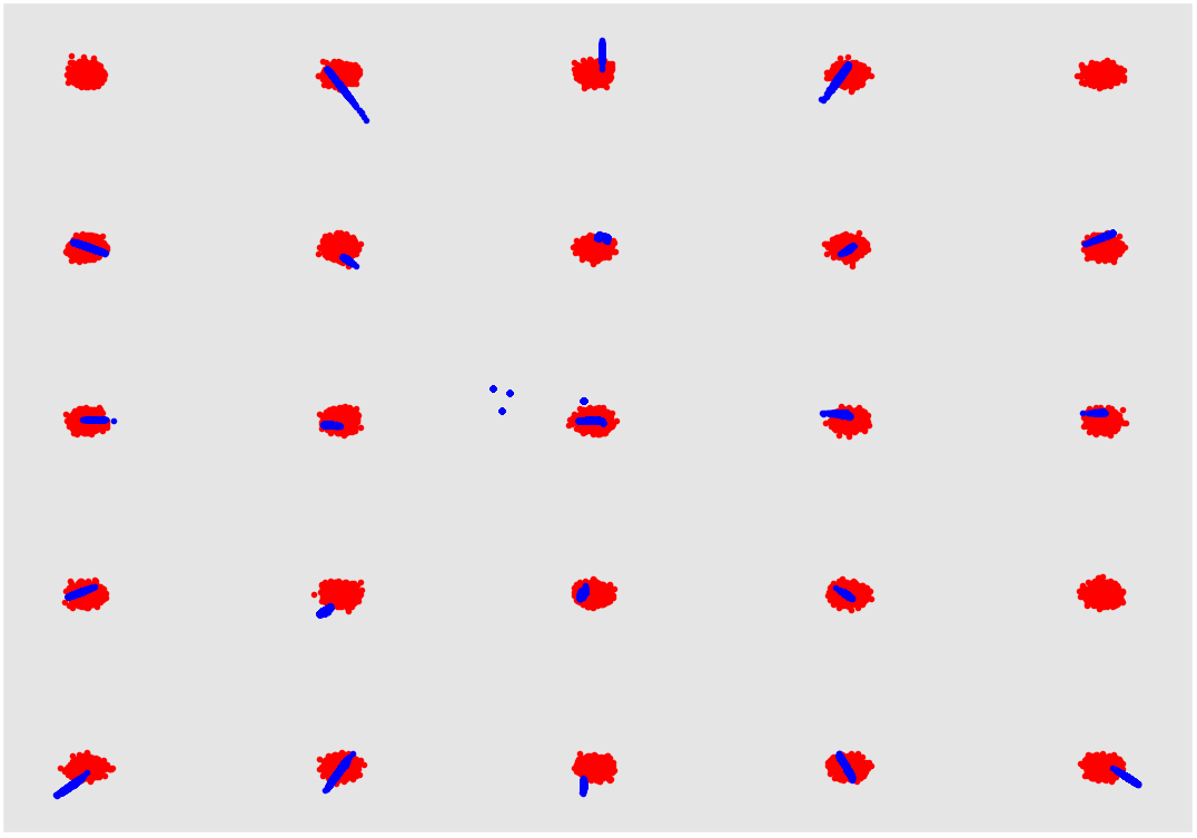
Figure 4: Left/right: visual comparison of generated samples on the 2D-grid dataset using PGMGAN, with/without architecture restriction for the space partitioner. The red/blue points illustrate the real/generated data samples. In the right plot, some modes are missed and their corresponding generators focus on the wrong area.

5.1 Toy dataset

This section aims to illustrate the importance of having a proper guide with no local optima. We also provide intuition about how our method helps GAN training. To that end, we use the canonical 2D-grid dataset, a mixture of 25 bivariate Gaussian with identical variance, and means covering the vertices of a square lattice.

For this toy example the data points are low dimensional, thus we skip the feature learning step and directly train the space partitioner $S$. We train our space partitioner using two different architectures: one sets its neural network architecture to a multi-layer fully connected network with ReLU activations, while the other follows the properties of architecture construction in Section 4.2. Once the two networks are trained, both successfully learn to put each Gaussian component in a different cluster, i.e., both get perfect clustering accuracy. Nonetheless, the guide functions obtained from each architecture behave significantly different.

Figure 3 provides the graph of $-R_{i}({\bm{x}})$ for the two space partitioners, where $i$ is the partition ID for the red Gaussian data samples in the corner. The right plot shows that $-R_{i}({\mathbf{x}})$ can have undesired local optima when the conditions of Section 4.2 are not enforced. Therefore, a universal reliable gradient is not provided to move the data samples toward the partition of interest. On the other hand, when the guide’s architecture follows these conditions (left plot), taking the direction of $\nabla-R_{i}({\bm{x}})$ guarantees reaching to partition $i$.

Figure 4 shows the effect of both these guides in the training of our mixture of generators using Equation 4.2. As shown, when $R_{i}$ has local optima, the generator of that region may get stuck in those local optima and miss the desired mode. As shown in Liu et al. [46] and the Appendix, GANs trained with no guide also fail to generate all the modes in this dataset. Furthermore, in contrast to standard GANs, we don’t generate samples from the space between different modes due to our partitioning and mixture of generators, mitigating the mode connecting problem. We provide empirical results for this dataset in the Appendix.

5.2 Stacked-MNIST, CIFAR-10 and STL-10

In this section, we conduct extensive experiments to evaluate the proposed Partition-Guided Mixture of Generators (PGMGAN) model. We also quantify the performance gains for the different parts of our method through an ablation study. We randomly generated the partition labels in one baseline to isolate the effect of proper partitioning from the architecture choice of $G_{i}$/$D_{i}$’s. We also ablate the benefits of the guide function by making a baseline where $\lambda=0$. For all experiments, we use $k=200$ unless specified otherwise.

Tables 1 and 2 presents our results on Stacked MNIST, CIFAR-10 and STL-10 respectively. From these tables, it is evident how training multiple generators using the space partitioner allows us to significantly outperform the other benchmark algorithms in terms of all metrics. Comparing Random Partition ID to Partition+GAN clearly shows the importance of having an effective partitioning in terms of performance and mode covering. Furthermore, the substantial gap between PGMGAN and Partition+GAN empirically demonstrates the value of utilizing the guide term.

Table 2: Unsupervised image generation results on STL-10. The results of all compared method are taken from Tian et al. [73]

	STL-10
	FID $\downarrow$	IS $\uparrow$
D2GAN [58]	-	7.98
DFM [79]	-	8.51
ProbGAN [23]	46.74	8.87
SN-GAN [55]	40.15	9.10
Dist-GAN [74]	36.19	-
MGAN [27]	-	9.22
Improved MMD [77]	37.63	9.34
AGAN [76]	52.75	9.23
AutoGAN [19]	31.01	9.16
E2GAN [73]	25.35	9.51
Partition GAN (Ours)	26.28	10.35
PGMGAN (Ours)	19.52	11.16

We first perform overall comparisons against other recent GANs. As shown in Table 2, PGMGAN achieves state-of-the-art FID and IS on the STL-10 dataset. Furthermore, PGMGAN outperforms several other baseline models, even over supervised class-conditional GANs, on both CIFAR-10 and Stacked-MNIST, as shown in Table 1. The significant improvements of FID and IS reflect the large gains in diversity and image quality on these datasets.

Following Liu et al. [46], we calculate the reverse KL metric using pre-trained classifiers to classify and count the occurrences of each mode for both Stacked-MNIST and CIFAR-10. These experiments and comparisons demonstrate that our proposed guide model effectively improves the performance of GANs in terms of mode collapse.

5.3 Image generation on unsupervised ImageNet

To show that our method remains effective on a larger more complex dataset, we also evaluated our model on unsupervised ILRSVRC2012 (ImageNet) dataset which contains roughly 1.2 million images with 1000 distinct categories; we down-sample the images to 128$\times$128 resolution for the experiment. We use $k=1000$ and adopt the architecture of BigGAN [5] for our generators and discriminators. Please see the Appendix for the details of experimental settings.

Our results are presented in Table 3. To the best of our knowledge, we achieve a new state of the art (SOTA) in unsupervised generation on ImagNet apart from augmentation based methods.

Table 3: FID and Inception Score (IS) metrics for unsupervised image generation on ImageNet at resolution 128$\times$128. The results of all compared methods are taken from Liu et al. [46]

	ImageNet
	FID $\downarrow$	IS $\uparrow$
GAN [20]	54.17	14.01
PacGAN2 [45]	57.51	13.50
PacGAN3 [45]	66.97	12.34
MGAN [27]	58.88	13.22
RotNet Feature Clustering	53.75	13.76
Logo-GAN-AE [65]	50.90	14.44
Self-Cond-GAN [46]	40.30	15.82
PGMGAN (Ours)	21.73	23.31

5.4 Parameter sensitivity

Additionally, we study the sensitivity of our overall PGMGAN method to the choice of guide’s weight $\lambda$ (Eq. 4.2), and number of clusters $k$. Figure 5 shows the results with varying $\lambda$ over CIFAR-10, demonstrating that our method is relatively robust to the choice of this hyper-parameter. Next, we change $k$ for a fixed $\lambda=6.0$ and report the results in Table 4. we observe that our method performs well for a wide range of $k$.

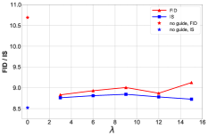
Figure 5: Effect of changing the guide’s weight $\lambda$ in equation 4.2 on PGMGAN performance. $\lambda=0$ corresponds to the partition+GAN.

Table 4: Effect of number of partitions ($k$) on PGMGAN performance. Results are averaged over five random trials, with standard error reported.

	CIFAR-10
	FID $\downarrow$	IS $\uparrow$
GAN [20]	$28.08\pm 0.47$	${6.98}\pm 0.06$
PGMGAN ($k=50$)	${9.27}\pm 0.45$	${8.69}\pm 0.07$
PGMGAN ($k=100$)	${8.97}\pm 0.33$	${8.75}\pm 0.05$
PGMGAN ($k=200$)	${8.93}\pm 0.38$	${8.81}\pm 0.10$
Class Conditional GAN [54]	${23.56}\pm 2.24$	${7.44}\pm 0.08$

6 Conclusion

We introduce a differentiable space partitioner to alleviate the GAN training problems, including mode connecting and mode collapse. The intuition behind how this works is twofold. The first reason is that an efficient partitioning makes the distribution on each region simpler, making its approximation easier. Thus, we can have a better approximation as a whole, which can alleviate both mode collapse and connecting problems. The second intuition is that the space partitioner can provide extra gradient, assisting the discriminator in training the mixture of generators. This is especially helpful when the discriminator’s gradient is unreliable. However, it is crucial to have theoretical guarantees that this extra gradient does not deteriorate the GAN training convergence in any way. We identify a sufficient theoretical condition for the space partitioner (in the functional space), and we realize that condition empirically by an architecture design for the space partitioner. Our experiments on natural images show the proposed method improves existing ones in terms of both FID and IS. For future work, we would like to investigate using the space partitioner for the supervised regime, where each data label has its own partitioning. Designing a more flexible architecture for the space partitioner such that its guide function does not have local optima is another direction we hope to explore.

Appendix A Proofs

See 1

Proof.

We begin by re-stating the definition of Minkowski sum and proceed by proving the theorem for the case where the number of manifold is 2. To extend the theorem form $k=2$ to the general case, one only needs to consider manifold $\mathcal{M}_{i}$ as $\mathcal{M}_{1}$, and $\bigcup_{j\in[1:k]\setminus{i}}\mathcal{M}_{j}$ as $\mathcal{M}_{2}$.

Definition 1 (Minkowski sum).

The Minkowski sum of two sets $U,V\in{\mathbb{R}}^{d}$ defined as

$$U+V:=\{u+v|u\in U,v\in V\}$$

and when $V$ is a $d$ dimensional ball with radius $r$ and centered at zero, we use the notation $U_{r}$ to refer to their Minkowski sum.

If we let $U^{(1)}:=G_{\theta}^{-1}(\mathcal{M}_{1}),U^{(2)}:=G_{\theta}^{-1}(\mathcal{M}_{2})$, then:

$$\forall r_{1},r_{2}\in{\mathbb{R}}_{+},~{}\text{if}~{}~{}~{}r_{1}+r_{2}<d_{1}/c\implies U^{(1)}_{r_{1}}\cap U^{(2)}_{r_{2}}=\emptyset$$

that is because if there exists an ${\mathbf{x}}\in U^{(1)}_{r_{1}}\cap U^{(2)}_{r_{2}}$, there would be ${\mathbf{u}}_{1}\in U^{(1)},{\mathbf{u}}_{2}\in U^{(2)}$ such that:

However, due to lipsitz condition of $G_{\theta}$:

$$||G_{\theta}({\mathbf{u}}_{1})-G_{\theta}({\mathbf{u}}_{2})||<c||{\mathbf{u}}_{1}-{\mathbf{u}}_{2}||<c\cdot d_{1}/c=d_{1}$$

which contradicts with our assumption that the distance between $\mathcal{M}_{1},\mathcal{M}_{2}$ is $d_{1}$. Therefore there is no point in the intersection of $U^{(1)}_{r_{1}}$ and $U^{(2)}_{r_{2}}$. The disjointness of this two sets provides us:

$$\gamma_{n}(U^{(1)}_{r_{1}})+\gamma_{n}(U^{(2)}_{r_{2}})\leq\gamma_{n}({\mathbb{R}}^{n})=1$$

where $\gamma_{n}(.)$ of any set is the probability of a random draw of $\mathcal{N}(0,{\bm{I}}_{n})$ being from that set. We proceed by using a remark from theorem 1.3 of [42] which restated below:

Lemma 1.

If $U$ is a Borel set in ${\mathbb{R}}^{n}$, then:

$$p\leq\gamma_{n}(U)\implies\Phi(\Phi^{-1}(p)+r)\leq\gamma_{n}(U_{r}).$$

Based on above lemma if we let:

$$p_{1}:=\gamma_{n}(U^{(1)}),\;\;p_{2}:=\gamma_{n}(U^{(2)})$$

then for $\forall r_{1},r_{2}\in{\mathbb{R}}_{+}$ such that $r_{1}+r_{2}<d_{1}/c$, we have:

$$\Phi(\Phi^{-1}(p_{1})+r_{1})+\Phi(\Phi^{-1}(p_{2})+r_{2})\leq 1$$ (10)

We can now calculate the total variational distance of the marginal distributions of $p_{\rm{data}},\,p_{\rm{model}}$ on the set $\{G_{\theta}(U^{(1)}),G_{\theta}(U^{(2)}),G_{\theta}\left({\mathbb{R}}^{n}\setminus(U^{(1)}\cup U^{(2)})\right)\}$ as:

and since total variational distance takes a smaller value on marginal distributions than the full distribution, we only need to show that for any $i$ the expression in the equation 11 is larger than $g(\pi_{i},d_{i},c)$ to prove the theorem 1 for $k=2$. Here $g(\pi_{i},d_{i},c)=\pi_{i}^{*}-\Phi(\Phi^{-1}(\pi_{i}^{*})-d_{i}/c)$.

Assume $p_{1}\leq\pi_{1}$, and define $\Delta_{1}:=\pi_{1}-p_{1}\geq 0$, based on equation 10 if $r_{1}=d_{1}/c,\,\;r_{2}=0$, we have:

$$\Phi(\Phi^{-1}(\pi_{1}-\Delta_{1})+d_{1}/c)+p_{2}\leq 1$$

which based on equation 10 implies:

$$r(\Delta_{1}):=\Phi(\Phi^{-1}(\pi_{1}-\Delta_{1})+d_{1}/c)-(\pi_{1}-\Delta_{1})\leq D_{TV}$$

which $D_{TV}$ refers to total variational distance between the marginal distributions of the data and model. We also know from the equation 10, that $\Delta_{1}\leq D_{TV}$, therefore:

$$\max(r(\Delta_{1}),\Delta_{1})\leq D_{TV}$$

for a $\Delta_{1}\in[0,\pi_{1}]$. Therefore

$$\min_{\delta_{1}\in[0,\pi_{1}]}\{\max(r(\delta_{1}),\delta_{1})\}\leq D_{TV}$$

To find the $\delta_{1}$ which minimize the above equation, we need to check endpoints of the interval $[0,\pi_{1}]$, points where the curve of two functions $r(\delta_{1}),\delta_{1}$ intersects with each other, and points that are the local minimaum of each of them. It can be shown the function $r(\delta_{1})$ does not have any local minima when $0<\pi_{1}<1$ because:

$$r(\delta_{1})=P({\textnormal{z}}\in[\Phi^{-1}(\pi_{1}-\delta_{1}),\Phi^{-1}(\pi_{1}-\delta_{1})+d_{1}/c])$$ (12)

where z is univarite standard normal random variable. Therefore $r(\delta_{1})$ is the probablity of a univarite normal being in a fixed length interval $d_{1}/c$, and $\delta_{1}$ only changes the starting point of the interval. By using this fact, it can be easily shown this function does not have any local optima in the open interval $(0,\pi_{1})$. Also the identity function $\delta_{1}$ also has no local optima inside the interval. The endpoints values are:

$$\max(r(0),0)=\Phi(\Phi^{-1}(\pi_{1})+d_{1}/c)-\pi_{1}$$

$$\max(r(\pi_{1}),\pi_{1})=\max(\Phi(\Phi^{-1}(0)+d_{1}/c),\pi_{1})=\pi_{1}$$

The function curves of $r$ and identity also intersects only when:

$$\Phi(\Phi^{-1}(\pi_{1}-\delta_{1}^{*})+d_{1}/c)=\pi_{1}$$

which only happens when:

$$\pi_{1}-\Phi(\Phi^{-1}(\pi_{1})-d_{1}/c)=\delta_{1}^{*}$$

where for this point, $\max(r(\delta_{1}^{*}),\delta_{1}^{*})=\delta_{1}^{*}$. Therefore based on the above calculations:

$$\min\left\{\underbrace{\Phi(\Phi^{-1}(\pi_{1})+d_{1}/c)-\pi_{1}}_{\text{I}}\,,\,\pi_{1},\\ \underbrace{\pi_{1}-\Phi(\Phi^{-1}(\pi_{1})-d_{1}/c)}_{\text{II}}\right\}\leq D_{TV}$$

Note, $\pi_{1}$ is always smaller than term II, and term I (II) is equal to probability of a univariate standard normal random variable being inside the interval $[\Phi^{-1}(\pi_{1}),\Phi^{-1}(\pi_{1})+d_{1}/c]$ ($[\Phi^{-1}(\pi_{1})-d_{1}/c,\Phi^{-1}(\pi_{1})]$). This observation implies that term II is smaller than term I, if and only if $\pi_{1}\leq\pi_{2}$. Based on this fact and symmetry of $\Phi$ with respect to zero, it can be easily shown that:

$$g(\pi_{1},d_{1},c)\leq D_{TV}$$ (13)

which proves the theorem. However, we made an assumption that $p_{1}\leq\pi_{1}$, this does not harm the argument because otherwise we would have $p_{2}\leq\pi_{2}$, and we can restate all the above arguments for $\pi_{2}$ instead of $\pi_{1}$. And, since $\pi_{2}=1-\pi_{1}$ and $d_{1}=d_{2}$, therefore we can have $g(\pi_{1},d_{1},c)=g(\pi_{2},d_{2},c)$, which proves equation 13. ∎

See 2

Proof.

Based on the definition of the JSD, we have:

$${\rm JSD}(P\parallel Q)=\frac{1}{2}{\rm KL}(P\parallel\frac{P+Q}{2})+\frac{1}{2}{\rm KL}(Q\parallel\frac{P+Q}{2})$$

We also have:

$${\rm KL}(P\parallel \frac{P+Q}{2})=$$

$$\int_{{\mathbb{R}}^{d}} P(x)\log\frac{P(x)}{P(x)+Q(x)}\,dx+\log 2=$$

$$\sum_{i}\int_{{A}_{i}} P(x)\log\frac{P(x)}{P(x)+Q(x)}\,dx+\log 2=$$

$$\sum_{i}\int_{{A}_{i}} \pi_{i}p_{i}(x)\log\frac{\pi_{i}p_{i}(x)}{\pi_{i}p_{i}(x)+\pi_{i}q_{i}(x)}\,dx+\log 2=$$

$$\sum_{i}\pi_{i} (\int_{{A}_{i}}p_{i}(x)\log\frac{p_{i}(x)}{p_{i}(x)+q_{i}(x)}\,dx+\log 2)=$$

$$\sum_{i}\pi_{i}{\rm KL}(p_{i}\parallel\frac{p_{i}+q_{i}}{2}).$$

Therefore:

$${\rm KL}(P\parallel\frac{P+Q}{2})=\sum_{i}\pi_{i}{\rm KL}(p_{i}\parallel\frac{p_{i}+q_{i}}{2}),$$

and similarly:

$${\rm KL}(Q\parallel\frac{P+Q}{2})=\sum_{i}\pi_{i}{\rm KL}(q_{i}\parallel\frac{p_{i}+q_{i}}{2})$$

Adding these two terms completes the proof. ∎

See 3

Proof.

We start by proving that the Jacobian matrix of function $\phi$ is invertible for any ${\mathbf{x}}\in{\mathbb{R}}^{d}$. Since $\phi\in C^{1}$, based on Taylor’s expansion theorem for multi-variable vector-valued function $\phi$, we can write:

$$\phi({\mathbf{y}})-\phi({\mathbf{x}})={\bm{J}}_{\phi}({\mathbf{x}})\left({\mathbf{y}}-{\mathbf{x}}\right)+o\left(||{\mathbf{y}}-{\mathbf{x}}||\right)$$

Were $o(\cdot)$ is the Little-o notation. By taking norm from both sides and using triangle inequality, we have:

$$||\phi({\mathbf{y}})-\phi({\mathbf{x}})||\leq||{\bm{J}}_{\phi}({\mathbf{x}})\left({\mathbf{y}}-{\mathbf{x}}\right)||+||o\left(||{\mathbf{y}}-{\mathbf{x}}||\right)||$$

Also because:

$$c_{0}||{\mathbf{y}}-{\mathbf{x}}||\leq||\phi({\mathbf{y}})-\phi({\mathbf{x}})||$$

$$\implies c_{0}||{\mathbf{y}}-{\mathbf{x}}||\leq||{\bm{J}}_{\phi}({\mathbf{x}})\left({\mathbf{y}}-{\mathbf{x}}\right)||+||o\left(||{\mathbf{y}}-{\mathbf{x}}||\right)||$$ (14)

thus for any fixed ${\mathbf{x}}$: $\exists\,\epsilon>0$ such that $\forall\,{\mathbf{y}}\in{\mathbb{R}}^{d}$ where $||{\mathbf{y}}-{\mathbf{x}}||\leq\epsilon$ then:

$$||o\left(||{\mathbf{y}}-{\mathbf{x}}||\right)||\leq\frac{c_{0}}{2}||{\mathbf{y}}-{\mathbf{x}}||$$

which combined with the inequality 14, results in:

$$\frac{c_{0}}{2}||{\mathbf{y}}-{\mathbf{x}}||\leq||{\bm{J}}_{\phi}({\mathbf{x}})\left({\mathbf{y}}-{\mathbf{x}}\right)||$$

For ${\mathbf{y}}\neq{\mathbf{x}}$, let ${\mathbf{u}}:=({\mathbf{y}}-{\mathbf{x}})/||{\mathbf{y}}-{\mathbf{x}}||$, then by dividing both sides of the above inequality to $||{\mathbf{y}}-{\mathbf{x}}||$ we have:

$$\forall{\mathbf{u}}\in{\mathbb{R}}^{d},||{\mathbf{u}}||=1\implies\frac{c_{0}}{2}\leq||{\bm{J}}_{\phi}({\mathbf{x}}){\mathbf{u}}||$$

which shows the Jacobian matrix of $\phi$ is invertiable for any ${\mathbf{x}}$ and all of its singular values are larger than $c_{0}/2$. If there is no ${\mathbf{x}}\in{\mathbb{R}}^{d}\setminus A_{i}$ the proof is complete. Otherwise, consider any ${\mathbf{x}}\in{\mathbb{R}}^{d}\setminus A_{i}$, for this ${\mathbf{x}}$ we have:

$$0<R_{i}({\mathbf{x}})=\sum_{c}(f_{c}({\mathbf{x}})-f_{i}({\mathbf{x}}))_{+}=\sum_{c}(({\bm{w}}_{c}-{\bm{w}}_{i})\phi({\mathbf{x}}))_{+}$$

where ${\bm{w}}_{j}$ is the $j$’th row of the matrix ${\bm{W}}^{\textit{partitioner}}$. Let:

$$I({\mathbf{x}}):=\{c|f_{c}({\mathbf{x}})>f_{i}({\mathbf{x}}),~{}~{}~{}c\in[1:k]\}$$

which is an non-empty set, because $0<R_{i}({\mathbf{x}})$ and we have

$$0<R_{i}({\mathbf{x}})=\left[\sum_{c\in I({\mathbf{x}})}({\bm{w}}_{c}-{\bm{w}}_{i})\right]\phi({\mathbf{x}})$$

$$\implies{\bm{v}}:=\sum_{c\in I({\mathbf{x}})}({\bm{w}}_{c}-{\bm{w}}_{i})\neq 0$$

Taking the gradient of the new formulation of $R_{i}$, we have:

$$\nabla R_{i}({\mathbf{x}})=\left[\sum_{c\in I({\mathbf{x}})}({\bm{w}}_{c}-{\bm{w}}_{i})\right]\nabla(\phi({\mathbf{x}}))={\bm{v}}{\bm{J}}_{\phi}({\mathbf{x}})$$

but since we showed earlier that all of the singular values of the Jacobian matrix is larger than $c_{0}/2$, the Jacobian matrix is $d\times d$, and ${\bm{v}}$ is not equal to zero, it can be easily shown:

$$||\nabla R_{i}({\mathbf{x}})||>||{\bm{v}}||\frac{c_{0}}{2}:=b_{0}$$

Now, we also need to show ${A}_{i}$ is connected for any $i$ to complete the proof. To that end, we first show $\phi$ is a surjective function, which means its image is ${\mathbb{R}}^{d}$. To show the $\phi$ is surjective, we prove its image is both an open and closed set, then since the only sets which are both open and closed (in ${\mathbb{R}}^{d}$) are ${\mathbb{R}}^{d},\emptyset$, we can conclude the surejective property. The image of $\phi$ is an open set due to Inverse Function Theorem [62] for $\phi$. We are allowed to use Inverse Function Theorem, since $\phi$ satisfies both $C^{1}$ condition and non zero determinant for all the points in the domain. We will also show that the image of $\phi$ is a closed set by showing it contains all of its limit points. Let ${\bm{y}}$ be a limit point in the image of $\phi$, that is there exists $\{{\bm{x}}_{1},{\bm{x}}_{2},\cdots\}$ such that $\phi({\bm{x}}_{r})\to{\bm{y}}$. Since ${\mathbb{R}}^{d}$ is complete and we have $c_{0}||{\bm{x}}_{r}-{\bm{x}}_{s}||\leq||\phi({\bm{x}}_{r})-\phi({\bm{x}}_{s})||$, then $\{{\bm{x}}_{1},{\bm{x}}_{2},\cdots\}$ is a Cauchy sequence. Finally since $\phi$ is a continues function $\phi({\bm{x}}^{*})={\bm{y}}$, completing the proof.

The function $\phi$ is also an invertible function because if $\phi({\bm{x}})=\phi({\bm{y}})$ then

$$c_{0}||{\mathbf{x}}-{\bm{y}}||\leq||\phi({\bm{x}})-\phi({\bm{y}})||=0$$

which implies ${\bm{x}}={\bm{y}}$. Therefore $\phi$ is in fact a continuous bijecitve function, which means it has a continuous inverse defined on all the space ${\mathbb{R}}^{d}$. Furthermore, it can be easily shown $R_{i}$ for a datapoint is zero iff its transformation by $\phi$ lies in a polytope (where each of its facets is a hyperplance perpendicular to a ${\bm{w}}_{c}-{\bm{w}}_{i}$). Since convex polytope is a connected set, and by applying $\phi^{-1}$ (it is well defined everywhere because of bijective property of $\phi$) to it, we would have a connected set. That is because a continuous function does not change the connectivity and $\phi^{-1}$ is continuous. ∎

Appendix B Additional qualitative results

We present more samples of our method showing both the partitioner and generative model’s performance. Figure 6 and Figure 7 visualize the sample diversity and quality of our method on CIFAR-10 and STL-10.

B.1 CIFAR-10

    Real                    Generated

(a) Partition 1

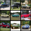
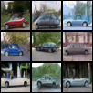
    Real                    Generated

(b) Partition 3

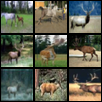
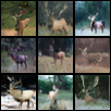
    Real                    Generated

(c) Partition 12

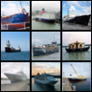
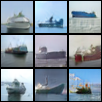
    Real                    Generated

(d) Partition 13

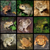
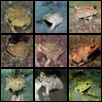
    Real                    Generated

(e) Partition 28

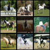
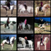
    Real                    Generated

(f) Partition 37

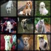
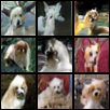
    Real                    Generated

(g) Partition 42

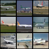
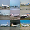
    Real                    Generated

(h) Partition 50

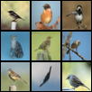
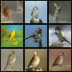
    Real                    Generated

(i) Partition 54

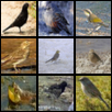
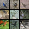
    Real                    Generated

(j) Partition 82

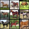
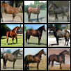
    Real                    Generated

(k) Partition 86

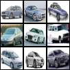
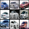
    Real                    Generated

(l) Partition 94

Figure 6: Extra examples of unsupervised partitioning and their corresponding real/generated samples on CIFAR-10 dataset.

B.2 STL-10

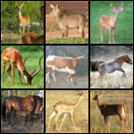
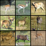
       Real                          Generated

(a) Partition 47

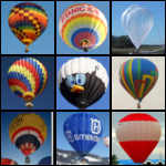
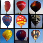
       Real                          Generated

(b) Partition 49

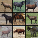
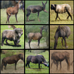
       Real                          Generated

(c) Partition 75

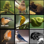
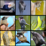
       Real                          Generated

(d) Partition 91

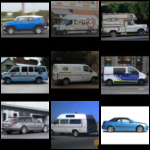
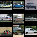
       Real                          Generated

(e) Partition 100

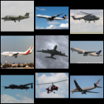
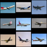
       Real                          Generated

(f) Partition 113

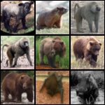
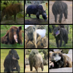
       Real                          Generated

(g) Partition 177

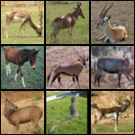
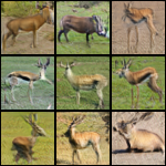
       Real                          Generated

(h) Partition 189

Figure 7: Extra examples of unsupervised partitioning and their corresponding real/generated samples on STL-10 dataset.

Appendix C Implementation details

We use two RTX 2080 Ti GPUs for experiments on STL-10, eight V-100 GPUs for ImageNet and a single GPU for all other experiments.

Space partitioner. For all experiments we use the same architecture for our space partitioner $S$. We use pre-activation Residual-Nets with 20 convolutional bottleneck blocks with 3 convolution layers each and kernel sizes of $3\times 3$, $1\times 1$, $3\times 3$ respectively and the ELU [11] nonlinearity. The network has 4 down-sampling stages, every 4 blocks where a dimension squeezing operation is used to decrease the spatial resolution. We use 160 channels for all the blocks. We do not use any initial padding due to our theoretical requirements. The negative slope of LeakyReLU is set as 0.2. In fact we can use a soft version of LeakyReLU if it is critical to guarantee the $C^{1}$ constraint of $\phi$. We train our pretext network for 500 epochs with momentum SGD and a weight decay of 3e-5, learning rate of $0.4$ with cosine scheduling, momentum of $0.9$, and batch size of 400 for CIFAR-10 and 200 for STL-10. The final space partitioner is trained for 100 epochs using Adam [38] with a learning rate of 1e-4 and batch size of 128. The weights in equation 4.1 are set to $\alpha=5$ and $\beta=$ 1e-3.

Generative model. Following SN-GANs [55] for image generation at resolution 32 or 48, we use the architectures described in Tables 6 and 7. Generators/discriminators are different from each other in first-layer/last-layer by having different partition ID embeddings, (which in fact acts as the condition). We use Adam optimizer with a batch size of 100. For the coefficient of guide $\lambda$ we utilized linear annealing during training, decreasing form 6.0 to 0.0001. Both $G$’s and $D$ networks are initialized with a normal $\mathcal{N}(0,0.02{\bm{I}})$. For all GAN’s experiments, we use Adam optimizer [38] with $\beta_{1}=0$, $\beta_{2}=0.999$ and a constant learning rate 2 for both $G$ and $D$. The number of $D$ steps per $G$ step training is 4.

For ImageNet experiment, we adopt the full version of BigGAN model architecture [5] described in Table 8. In this experiment, we apply the shared class embedding for each CBN layer in G, and feed noise $z$ to multiple layers of $G$ by concatenating with the partition ID embedding vector. Moreover, we add Self-Attention layer with the resolution of 64, and we employ orthogonal initialization for network parameters [67]. We use batch size of 256 and set the number of gradient accumulations to 8.

Evaluation. It has been shown that [10, 48] when the sample size is not large enough, both FID and IS are biased, therefor we use N=50,000 samples for computing both IS and FID metrics. We also use the official TensorFlow scripts for computing FID.

C.1 Additional Experiments:

Our quantitative results on the (2D-ring, 2D-grid) toy datasets [45] are: recovered modes: (8 , 25), high quality samples: (99.8 , 99.8), reverse KL: (0.0006, 0.0034).

Given the strong performances of recent models (and ours) on these datasets we suffice to these stats. For visualizations of our generated samples related to these two datasets please see Figure 4-left and refer to the appendix of [46] for other methods.

Additional architecture dependent experiment: Since SelfCondGAN [46] uses certain features from the discriminator, it is not trivial to adopt to other architectures. Thus, we trained PGMGAN with the same G/D architecture on CIFAR10 yielding an FID of 10.65.

Partitioning method One way to assess the quality of the space partitioner is by measuring its performance on placing semantically similar images in the same partition. To that end, we use the well-accepted clustering metric Normalized Mutual Information (NMI). NMI is a normalization of the Mutual Information (MI) between the true and inferred labels. This metric is invariant to permutation of the class/partition labels and is always between 0 and 1, with a higher value suggesting a higher quality of partitioning. Table 5 compares the clustering performance of our method to the-stat-of-the-art partition-based GAN method Liu et. [46], which clearly shows superiority of our method.

Table 5: Comparison of the clustering performance in term of Normalized Mutual Information (NMI), higher is better.

	Stacked MNIST	CIFAR-10	STL-10	ImageNet
Self-Cond-GAN [46]	0.3018	0.3326	-	17.39
PGMGAN	0.4805	0.4146	0.3911	68.57

Table 6: GANs architecture for $32\times 32$ images.

$z\in{\mathbb{R}}^{128}\sim\mathcal{N}(0,I)$

Embed(PartitionID) $\in{\mathbb{R}}^{128}$

dense, $4\times 4\times 256$

ResBlock up $256$

ResBlock up $256$

ResBlock up $256$

BN, ReLU, $3\times 3$ Conv, $3$ Tanh

(a) Generator

RGB image $x\in{\mathbb{R}}^{32\times 32\times 3}$

ResBlock down $128$

ResBlock down $128$

ResBlock $128$

ResBlock $128$

ReLU, Global sum pooling

Embed(PartitionID)$\cdot{\bm{h}}$ + (linear $\rightarrow$ 1)

(b) Discriminator

Table 7: GANs architecture for $48\times 48$ images.

$z\in{\mathbb{R}}^{128}\sim\mathcal{N}(0,I)$

Embed(PartitionID) $\in{\mathbb{R}}^{128}$

dense, $3\times 3\times 1024$

ResBlock up $512$

ResBlock up $256$

ResBlock up $128$

ResBlock up $64$

BN, ReLU, $3\times 3$ Conv, $3$ Tanh

(a) Generator

RGB image $x\in{\mathbb{R}}^{48\times 48\times 3}$

ResBlock down $64$

ResBlock down $128$

ResBlock down $256$

ResBlock down $512$

ResBlock $1024$

ReLU, Global sum pooling

Embed(PartitionID)$\cdot{\bm{h}}$ + (linear $\rightarrow$ 1)

(b) Discriminator

Table 8: GANs architecture for $128\times 128$ images. “$ch$” represents the channel width multiplier and is set to 96.

$z\in{\mathbb{R}}^{120}\sim\mathcal{N}(0,I)$

Embed(PartitionID) $\in{\mathbb{R}}^{128}$

Linear $(20+128)\rightarrow 4\times 4\times 16ch$

ResBlock up $16ch\rightarrow 16ch$

ResBlock up $16ch\rightarrow 8ch$

ResBlock up $8ch\rightarrow 4ch$

ResBlock up $4ch\rightarrow 2ch$

Non-Local Block ($64\times 64$)

ResBlock up $2ch\rightarrow ch$

BN, ReLU, $3\times 3$ Conv $ch\rightarrow 3$

Tanh

(a) Generator

RGB image $x\in{\mathbb{R}}^{128\times 128\times 3}$

ResBlock down $ch\rightarrow 2ch$

Non-Local Block ($64\times 64$)

ResBlock down $2ch\rightarrow 4ch$

ResBlock down $4ch\rightarrow 8ch$

ResBlock down $8ch\rightarrow 16ch$

ResBlock down $16ch\rightarrow 16ch$

ResBlock $16ch\rightarrow 16ch$

ReLU, Global sum pooling

Embed(PartitionID)$\cdot{\bm{h}}$ + (linear $\rightarrow$ 1)

(b) Discriminator

C.2 ImageNet

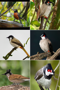
(a) Partition 034

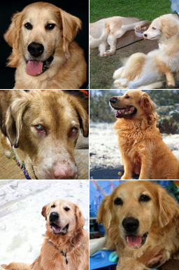
(b) Partition 159

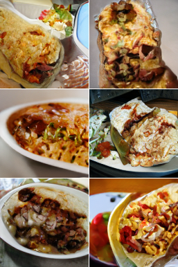
(c) Partition 455

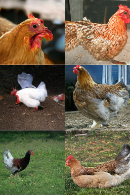
(d) Partition 642

Figure 8: Examples of generated samples on unsupervised ImageNet 128$\times$128 dataset.

References

- [1] Martin Arjovsky, Soumith Chintala, and Léon Bottou. Wasserstein generative adversarial networks. In International Conference on Machine Learning, 2017.
- [2] Samaneh Azadi, Catherine Olsson, Trevor Darrell, Ian Goodfellow, and Augustus Odena. Discriminator rejection sampling. International Conference on Learning Representations, 2019.
- [3] Jens Behrmann, Will Grathwohl, Ricky TQ Chen, David Duvenaud, and Jörn-Henrik Jacobsen. Invertible residual networks. In International Conference on Machine Learning, pages 573–582, 2019.
- [4] Ali Borji. Pros and cons of gan evaluation measures. Computer Vision and Image Understanding, 179:41–65, 2019.
- [5] Andrew Brock, Jeff Donahue, and Karen Simonyan. Large scale gan training for high fidelity natural image synthesis. In International Conference on Learning Representations, 2019.
- [6] Mathilde Caron, Piotr Bojanowski, Armand Joulin, and Matthijs Douze. Deep clustering for unsupervised learning of visual features. In Proceedings of the European Conference on Computer Vision (ECCV), pages 132–149, 2018.
- [7] Ting Chen, Simon Kornblith, Mohammad Norouzi, and Geoffrey Hinton. A simple framework for contrastive learning of visual representations. 2020.
- [8] Ting Chen, Simon Kornblith, Kevin Swersky, Mohammad Norouzi, and Geoffrey Hinton. Big self-supervised models are strong semi-supervised learners. arXiv preprint arXiv:2006.10029, 2020.
- [9] Ting Chen, Xiaohua Zhai, Marvin Ritter, Mario Lucic, and Neil Houlsby. Self-supervised gans via auxiliary rotation loss. In Proceedings of the IEEE Conference on Computer Vision and Pattern Recognition, pages 12154–12163, 2019.
- [10] Min Jin Chong and David Forsyth. Effectively unbiased fid and inception score and where to find them. In Proceedings of the IEEE/CVF Conference on Computer Vision and Pattern Recognition, pages 6070–6079, 2020.
- [11] Djork-Arné Clevert, Thomas Unterthiner, and Sepp Hochreiter. Fast and accurate deep network learning by exponential linear units (elus). In 4th International Conference on Learning Representations, ICLR 2016, San Juan, Puerto Rico, May 2-4, 2016, Conference Track Proceedings, 2016.
- [12] Adam Coates, Andrew Ng, and Honglak Lee. An Analysis of Single Layer Networks in Unsupervised Feature Learning. In AISTATS, 2011. https://cs.stanford.edu/~acoates/papers/coatesleeng_aistats_2011.pdf.
- [13] Emily L Denton, Soumith Chintala, Rob Fergus, et al. Deep generative image models using a laplacian pyramid of adversarial networks. In Advances in neural information processing systems, pages 1486–1494, 2015.
- [14] Jeff Donahue, Philipp Krähenbühl, and Trevor Darrell. Adversarial feature learning. In International Conference on Learning Representations, 2017.
- [15] Vincent Dumoulin, Ishmael Belghazi, Ben Poole, Olivier Mastropietro, Alex Lamb, Martin Arjovsky, and Aaron Courville. Adversarially learned inference. In International Conference on Learning Representations, 2017.
- [16] Carlos Florensa, David Held, Xinyang Geng, and Pieter Abbeel. Automatic goal generation for reinforcement learning agents. In ICML, 2018.
- [17] Spyros Gidaris, Praveer Singh, and Nikos Komodakis. Unsupervised representation learning by predicting image rotations. International Conference on Learning Representations, 2018.
- [18] Mingming Gong, Yanwu Xu, Chunyuan Li, Kun Zhang, and Kayhan Batmanghelich. Twin auxilary classifiers gan. In Advances in neural information processing systems, pages 1330–1339, 2019.
- [19] Xinyu Gong, Shiyu Chang, Yifan Jiang, and Zhangyang Wang. Autogan: Neural architecture search for generative adversarial networks. In Proceedings of the IEEE International Conference on Computer Vision, pages 3224–3234, 2019.
- [20] Ian Goodfellow, Jean Pouget-Abadie, Mehdi Mirza, Bing Xu, David Warde-Farley, Sherjil Ozair, Aaron Courville, and Yoshua Bengio. Generative adversarial nets. In Advances in Neural Information Processing Systems, 2014.
- [21] Ishaan Gulrajani, Faruk Ahmed, Martin Arjovsky, Vincent Dumoulin, and Aaron C Courville. Improved training of wasserstein gans. In Advances in Neural Information Processing Systems, 2017.
- [22] Swaminathan Gurumurthy, Ravi Kiran Sarvadevabhatla, and R Venkatesh Babu. Deligan: Generative adversarial networks for diverse and limited data. In The IEEE Conference on Computer Vision and Pattern Recognition (CVPR), 2017.
- [23] Hao He, Hao Wang, Guang-He Lee, and Yonglong Tian. Probgan: Towards probabilistic gan with theoretical guarantees, 2019.
- [24] Kaiming He, Haoqi Fan, Yuxin Wu, Saining Xie, and Ross Girshick. Momentum contrast for unsupervised visual representation learning. In Proceedings of the IEEE/CVF Conference on Computer Vision and Pattern Recognition, pages 9729–9738, 2020.
- [25] Kaiming He, Xiangyu Zhang, Shaoqing Ren, and Jian Sun. Deep residual learning for image recognition. In Proceedings of the IEEE conference on computer vision and pattern recognition, pages 770–778, 2016.
- [26] Martin Heusel, Hubert Ramsauer, Thomas Unterthiner, Bernhard Nessler, and Sepp Hochreiter. Gans trained by a two time-scale update rule converge to a local nash equilibrium. In Advances in Neural Information Processing Systems, pages 6626–6637, 2017.
- [27] Quan Hoang, Tu Dinh Nguyen, Trung Le, and Dinh Phung. Mgan: Training generative adversarial nets with multiple generators. In International Conference on Learning Representations, 2018.
- [28] Judy Hoffman, Eric Tzeng, Taesung Park, Jun-Yan Zhu, Phillip Isola, Kate Saenko, Alexei Efros, and Trevor Darrell. Cycada: Cycle-consistent adversarial domain adaptation. In International conference on machine learning, pages 1989–1998. PMLR, 2018.
- [29] Xun Huang, Ming-Yu Liu, Serge Belongie, and Jan Kautz. Multimodal unsupervised image-to-image translation. In Proceedings of the European Conference on Computer Vision (ECCV), pages 172–189, 2018.
- [30] Phillip Isola, Jun-Yan Zhu, Tinghui Zhou, and Alexei A Efros. Image-to-image translation with conditional adversarial networks. In Proceedings of the IEEE Conference on Computer Vision and Pattern Recognition, pages 1125–1134, 2017.
- [31] Tero Karras, Timo Aila, Samuli Laine, and Jaakko Lehtinen. Progressive growing of gans for improved quality, stability, and variation. ICLR, 2018.
- [32] Tero Karras, Miika Aittala, Janne Hellsten, Samuli Laine, Jaakko Lehtinen, and Timo Aila. Training generative adversarial networks with limited data. Advances in Neural Information Processing Systems, 2020.
- [33] Tero Karras, Samuli Laine, and Timo Aila. A style-based generator architecture for generative adversarial networks. In Proceedings of the IEEE conference on computer vision and pattern recognition, pages 4401–4410, 2019.
- [34] Tero Karras, Samuli Laine, Miika Aittala, Janne Hellsten, Jaakko Lehtinen, and Timo Aila. Analyzing and improving the image quality of stylegan. In Proceedings of the IEEE/CVF Conference on Computer Vision and Pattern Recognition, pages 8110–8119, 2020.
- [35] John L Kelley. General topology. Courier Dover Publications, 2017.
- [36] Mahyar Khayatkhoei, Maneesh Singh, and Ahmed Elgammal. Disconnected manifold learning for generative adversarial networks. arXiv preprint arXiv:1806.00880, 2018.
- [37] Nathan Killoran, Leo J Lee, Andrew Delong, David Duvenaud, and Brendan J Frey. Generating and designing dna with deep generative models. 2017.
- [38] Diederik P Kingma and Jimmy Ba. Adam: A method for stochastic optimization. arXiv preprint arXiv:1412.6980, 2014.
- [39] Alex Krizhevsky, Geoffrey Hinton, et al. Learning multiple layers of features from tiny images. 2009.
- [40] Jogendra Nath Kundu, Maharshi Gor, Dakshit Agrawal, and R Venkatesh Babu. Gan-tree: An incrementally learned hierarchical generative framework for multi-modal data distributions. In Proceedings of the IEEE International Conference on Computer Vision, pages 8191–8200, 2019.
- [41] Yann LeCun, Corinna Cortes, and CJ Burges. Mnist handwritten digit database. ATT Labs [Online]. Available: http://yann.lecun.com/exdb/mnist, 2, 2010.
- [42] Michel Ledoux. Isoperimetry and gaussian analysis. In Lectures on probability theory and statistics, pages 165–294. Springer, 1996.
- [43] Jiwei Li, Will Monroe, Tianlin Shi, Sébastien Jean, Alan Ritter, and Dan Jurafsky. Adversarial learning for neural dialogue generation. arXiv preprint arXiv:1701.06547, 2017.
- [44] Kevin Lin, Dianqi Li, Xiaodong He, Zhengyou Zhang, and Ming-Ting Sun. Adversarial ranking for language generation. In Advances in Neural Information Processing Systems, 2017.
- [45] Zinan Lin, Ashish Khetan, Giulia Fanti, and Sewoong Oh. Pacgan: The power of two samples in generative adversarial networks. In Advances in neural information processing systems, pages 1498–1507, 2018.
- [46] Steven Liu, Tongzhou Wang, David Bau, Jun-Yan Zhu, and Antonio Torralba. Diverse image generation via self-conditioned gans. In Proceedings of the IEEE/CVF Conference on Computer Vision and Pattern Recognition, pages 14286–14295, 2020.
- [47] Shaohui Liu, Xiao Zhang, Jianqiao Wangni, and Jianbo Shi. Normalized diversification. In Proceedings of the IEEE/CVF Conference on Computer Vision and Pattern Recognition, pages 10306–10315, 2019.
- [48] Mario Lucic, Karol Kurach, Marcin Michalski, Sylvain Gelly, and Olivier Bousquet. Are gans created equal? a large-scale study. In Advances in neural information processing systems, pages 700–709, 2018.
- [49] Mario Lucic, Michael Tschannen, Marvin Ritter, Xiaohua Zhai, Olivier Bachem, and Sylvain Gelly. High-fidelity image generation with fewer labels. International conference on machine learning, 2019.
- [50] Xudong Mao, Qing Li, Haoran Xie, Raymond YK Lau, Zhen Wang, and Stephen Paul Smolley. Least squares generative adversarial networks. In Proceedings of the IEEE international conference on computer vision, pages 2794–2802, 2017.
- [51] Mohamed Marouf, Pierre Machart, Vikas Bansal, Christoph Kilian, Daniel S Magruder, Christian F Krebs, and Stefan Bonn. Realistic in silico generation and augmentation of single-cell rna-seq data using generative adversarial networks. Nature communications, 11(1):1–12, 2020.
- [52] Lars Mescheder, Andreas Geiger, and Sebastian Nowozin. Which training methods for gans do actually converge? In International Conference on Machine Learning, pages 3478–3487, 2018.
- [53] Luke Metz, Ben Poole, David Pfau, and Jascha Sohl-Dickstein. Unrolled generative adversarial networks. International Conference on Learning Representations, 2017.
- [54] Mehdi Mirza and Simon Osindero. Conditional generative adversarial nets. arXiv preprint arXiv:1411.1784, 2014.
- [55] Takeru Miyato, Toshiki Kataoka, Masanori Koyama, and Yuichi Yoshida. Spectral normalization for generative adversarial networks. arXiv preprint arXiv:1802.05957, 2018.
- [56] Takeru Miyato and Masanori Koyama. cgans with projection discriminator. International Conference on Learning Representations, 2018.
- [57] Hariharan Narayanan and Sanjoy Mitter. Sample complexity of testing the manifold hypothesis. In Advances in neural information processing systems, pages 1786–1794, 2010.
- [58] Tu Nguyen, Trung Le, Hung Vu, and Dinh Phung. Dual discriminator generative adversarial nets. In Advances in Neural Information Processing Systems, pages 2670–2680, 2017.
- [59] Augustus Odena, Christopher Olah, and Jonathon Shlens. Conditional image synthesis with auxiliary classifier gans. In International conference on machine learning, pages 2642–2651, 2017.
- [60] Santiago Pascual, Antonio Bonafonte, and Joan Serrà. Segan: Speech enhancement generative adversarial network. Proc. Interspeech 2017, pages 3642–3646, 2017.
- [61] Alec Radford, Luke Metz, and Soumith Chintala. Unsupervised representation learning with deep convolutional generative adversarial networks. arXiv preprint arXiv:1511.06434, 2015.
- [62] Walter Rudin et al. Principles of mathematical analysis, volume 3. McGraw-hill New York, 1964.
- [63] Olga Russakovsky, Jia Deng, Hao Su, Jonathan Krause, Sanjeev Satheesh, Sean Ma, Zhiheng Huang, Andrej Karpathy, Aditya Khosla, Michael Bernstein, et al. Imagenet large scale visual recognition challenge. International journal of computer vision, 115(3):211–252, 2015.
- [64] Amir Sadeghian, Vineet Kosaraju, Ali Sadeghian, Noriaki Hirose, Hamid Rezatofighi, and Silvio Savarese. Sophie: An attentive gan for predicting paths compliant to social and physical constraints. In Proceedings of the IEEE/CVF Conference on Computer Vision and Pattern Recognition, pages 1349–1358, 2019.
- [65] Alexander Sage, Eirikur Agustsson, Radu Timofte, and Luc Van Gool. Logo synthesis and manipulation with clustered generative adversarial networks. In Proceedings of the IEEE Conference on Computer Vision and Pattern Recognition, pages 5879–5888, 2018.
- [66] Mehdi SM Sajjadi, Olivier Bachem, Mario Lucic, Olivier Bousquet, and Sylvain Gelly. Assessing generative models via precision and recall. In Advances in Neural Information Processing Systems, pages 5228–5237, 2018.
- [67] Tim Salimans, Ian Goodfellow, Wojciech Zaremba, Vicki Cheung, Alec Radford, and Xi Chen. Improved techniques for training gans. In Advances in Neural Information Processing Systems, 2016.
- [68] Thomas Schlegl, Philipp Seeböck, Sebastian M Waldstein, Ursula Schmidt-Erfurth, and Georg Langs. Unsupervised anomaly detection with generative adversarial networks to guide marker discovery. In International conference on information processing in medical imaging, pages 146–157. Springer, 2017.
- [69] Rui Shu, Hung Bui, and Stefano Ermon. Ac-gan learns a biased distribution. In NIPS Workshop on Bayesian Deep Learning, 2017.
- [70] Akash Srivastava, Lazar Valkoz, Chris Russell, Michael U Gutmann, and Charles Sutton. Veegan: Reducing mode collapse in gans using implicit variational learning. In Advances in Neural Information Processing Systems, pages 3308–3318, 2017.
- [71] Ugo Tanielian, Thibaut Issenhuth, Elvis Dohmatob, and Jeremie Mary. Learning disconnected manifolds: a no gans land. 2020.
- [72] Joshua B Tenenbaum, Vin De Silva, and John C Langford. A global geometric framework for nonlinear dimensionality reduction. science, 290(5500):2319–2323, 2000.
- [73] Yuan Tian, Qin Wang, Zhiwu Huang, Wen Li, Dengxin Dai, Minghao Yang, Jun Wang, and Olga Fink. Off-policy reinforcement learning for efficient and effective gan architecture search. ECCV, 2020.
- [74] Ngoc-Trung Tran, Tuan-Anh Bui, and Ngai-Man Cheung. Dist-gan: An improved gan using distance constraints. In Proceedings of the European Conference on Computer Vision (ECCV), pages 370–385, 2018.
- [75] Wouter Van Gansbeke, Simon Vandenhende, Stamatios Georgoulis, Marc Proesmans, and Luc Van Gool. Scan: Learning to classify images without labels. In European Conference on Computer Vision (ECCV), 2020.
- [76] Hanchao Wang and Jun Huan. Agan: Towards automated design of generative adversarial networks. arXiv preprint arXiv:1906.11080, 2019.
- [77] Wei Wang, Yuan Sun, and Saman Halgamuge. Improving MMD-GAN training with repulsive loss function. In International Conference on Learning Representations, 2019.
- [78] Xiaolong Wang and Abhinav Gupta. Generative image modeling using style and structure adversarial networks. In European conference on computer vision, pages 318–335. Springer, 2016.
- [79] David Warde-Farley and Yoshua Bengio. Improving generative adversarial networks with denoising feature matching. 2016.
- [80] Chang Xiao, Peilin Zhong, and Changxi Zheng. Bourgan: Generative networks with metric embeddings. NIPS, 2018.
- [81] Lantao Yu, Weinan Zhang, Jun Wang, and Yong Yu. Seqgan: Sequence generative adversarial nets with policy gradient. In Thirty-first AAAI conference on artificial intelligence, 2017.
- [82] Han Zhang, Ian Goodfellow, Dimitris Metaxas, and Augustus Odena. Self-attention generative adversarial networks. In International Conference on Machine Learning, pages 7354–7363. PMLR, 2019.
- [83] Han Zhang, Tao Xu, Hongsheng Li, Shaoting Zhang, Xiaogang Wang, Xiaolei Huang, and Dimitris N Metaxas. Stackgan: Text to photo-realistic image synthesis with stacked generative adversarial networks. In Proceedings of the IEEE international conference on computer vision, pages 5907–5915, 2017.
- [84] Han Zhang, Zizhao Zhang, Augustus Odena, and Honglak Lee. Consistency regularization for generative adversarial networks. International Conference on Learning Representations, 2020.
- [85] Zhengli Zhao, Zizhao Zhang, Ting Chen, Sameer Singh, and Han Zhang. Image augmentations for gan training. arXiv preprint arXiv:2006.02595, 2020.
- [86] Jun-Yan Zhu, Taesung Park, Phillip Isola, and Alexei A Efros. Unpaired image-to-image translation using cycle-consistent adversarial networks. In ICCV, 2017.