SMORES-EP, a Modular Robot with Parallel Self-assembly

Abstract

Self-assembly of modular robotic systems enables the construction of complex robotic configurations to adapt to different tasks. This paper presents a framework for SMORES types of modular robots to efficiently self-assemble into tree topologies. These modular robots form kinematic chains that have been shown to be capable of a large variety of manipulation and locomotion tasks, yet they can reconfigure using a mobile reconfiguration. A desired kinematic topology can be mapped onto a planar pattern with optimal module assignment based on the modules’ locations, then the mobile reconfiguration assembly process can be executed in parallel. A docking controller is developed to guarantee the success of docking processes. A hybrid control architecture is designed to handle a large number of modules and complex behaviors of each individual, and achieve efficient and robust self-assembly actions. The framework is demonstrated in both hardware and simulation on the SMORES-EP platform.

1 Introduction

It is common in nature that groups of individuals can join together to overcome the limited capability of individuals, especially for insects who often need to collaborate in large groups to accomplish tasks. This collective behavior in nature has inspired similar approaches for robotic systems. Modular robots are composed of numerous simple building blocks, or modules, that can be joined into different connected morphologies depending on task requirements. Determining the sequence of motions to form a goal configuration of modules is called self-assembly planning (Seo et al., 2016).

Self-assembly is related to self-reconfiguration for modular robots. There are in general three styles of self-reconfiguration among the variety of self-reconfigurable robot architectures: lattice, chain and mobile style (Yim et al., 2007a). Lattice style (Chirikjian, 1994) reconfiguration occurs with modules rearranging themselves to positions on a virtual lattice while maintaining a single connected component. Chain style (Yim et al., 2000) occurs between modules forming kinematic chains (links are connected by joints) again in a single connected component. The mobile style (Fukuda et al., 1991) occurs where modules can separate from each other and move on the environment before joining. Self-assembly is most related to the mobile style reconfiguration as pieces are assembled as separate units.

A particularly useful self-assembly example collaborative behavior can be shown for systems that can achieve mobile reconfiguration. Each individual module can locomote around an area, however it may discover it cannot cross a gap that is larger than one module. Instead multiple modules can join to form a snake configuration making it long enough to cross over. Other applications include reaching tall spaces or rapid simultaneous exploration. All of these behaviors are similar to the behaviors shown in ants.

An individual module usually has limited motion capability due to its design. Our goal is to allow modular robots to self-assemble into desired morphologies to perform complex tasks, such as dexterous manipulation, climbing stairs, navigation over complex terrains, and quick exploration. An individual module is not capable of handling these tasks because of its motion limitations. There are several challenges needed to be addressed:

1. Efficiency is important, especially for modular robotic systems that include a large number of modules;

2. Physical constraints have to be considered for real hardware applications;

3. Accurate docking is required.

Many modules can be involved in order to handle various scenarios and an efficient framework is important. The framework should output efficient assembly sequences and also provide an efficient architecture to control modules so that actions can be executed efficiently. A motion controller is necessary to accurately command multiple modules to move around with the hardware performance and motion constraints being considered. Docking actions have to be carefully executed and some connection can be coupled with module motions.

One example of a modular reconfigurable robot is the SMORES (Davey et al., 2012) and SMORES-EP systems. SMORES-EP uses EP-Face connectors (Tosun et al., 2016). Each SMORES module has four active rotational degrees-of-freedom (DOF), pan, tilt, and left/right wheels. It has differential wheeled drive using its left and right wheels. The SMORES modules are unique among self-reconfigurable systems in that they can reconfigure in any of the three styles noted earlier. The modules are individually mobile with the wheels. The system can form serial chains which has been shown to be one of the more useful configurations for doing things like manipulation of objects (Liu and Yim, 2020) or different styles of locomotion. While lattice style reconfiguration mechanisms have been studied in depth (Stoy, 2006), the mobile form of reconfiguration similar to self-assembly has not been.

In this paper, a parallel self-assembly algorithm for kinematic topologies (the connectivity of the modules) as well as controllers for hardware execution are presented using SMORES-EP modules. A target kinematic structure can be simply defined as a graph where each vertex is a module and each edge is the connection between adjacent modules. Given the current locations of all modules, every individual is mapped to a module in the target configuration in an optimal way with respect to some predefined cost (e.g. the total moving distance) by solving a task assignment problem. Then the assembly actions can be executed in parallel for efficiency while satisfying the physical hardware constraints. Docking is difficult for modular robots and a motion controller is also developed to guarantee the success of docking process. The control architecture of our system is hybrid: distributed at low level actions and centralized at high level planning. In our system, each SMORES-EP module has its own processor to handle hardware-level control and communication, and a central computer is used for tracking modules’ poses and high-level control and planning. This architecture makes use of distributed computing power and also achieves efficiency for communication and planning through centralized information processing. The effectiveness and robustness of the framework is demonstrated in both the simulation environment and the real world. Three tasks are presented and every task contains two simulation tests and one hardware test. The proposed framework can be easily extended to other mobile type modular robots as long as the topology is defined.

The paper is organized as follows. Section 2 reviews relevant work on self-assembly with modular robots. Section 3 introduces the hardware and software we developed to achieve robust self-assembly activities. Section 4 discusses some concepts and mathematical models that are necessary to describe a modular robot configuration and claims our self-assembly problem. The parallel assembly algorithm is presented in Section 5 as well as the controller to ensure the docking process. Three hardware experiments are shown in Section 6 to demonstrate the effectiveness of our framework. Finally, Section 7 concludes and presents future work.

2 Related Work

Modular robots have been an active research field over several decades, and a general review of these systems is done by Seo et al. (2019).

2.1 Modular Robots with Self-assembly

Various modular robotic systems have been developed with self-assembly capability. For mobile self-reconfiguration, CEBOT is one of the first (Fukuda et al., 1991), with a heterogeneous system composed of modules (cells) with different functions, such as mobile cells, bending joint cells, rotating joint cells, and sliding joint cells. The mobile cells are able to approach stationary cells for docking using a cone-shaped coupling mechanism so as to further self-assemble into a manipulation structure. However, its flexibility is limited to the single function and motion capability of each module. SMC Rover (Motomura et al., 2005) is a similar heterogeneous system that consists of one main body and multiple wheel units. The main body is stationary and equipped with some functional components (e.g. solar battery cells). Each wheel unit has a wheel for locomotion and an arm for manipulation. These wheel units can dock with the main body to form a vehicle or undock to execute missions by themselves.

Gunryu (Hirose et al., 1996) is a robotic system composed of multiple mobile vehicles and each vehicle has an arm installed as a connecting mechanism. These vehicles can be connected as snake-like robots to enhance the locomotion capability of the system, such as moving over a cliff and climbing stairs. A similar system is presented in (Brown et al., 2002) but using a simpler docking mechanism. Their docking capability can extend their applications but the morphologies formed are limited to single chain topology. Swarm-bot (Groß et al., 2006) modules also use robotic arms as a connecting mechanism, but are equipped with a surrounding ring for mating with grippers, which enables a module to link with more than one modules. However, the assembly behavior is limited to simple 2-dimensional structure for cooperative locomotion due to the shape of its modules. They cannot form dextrous kinematics structures to perform manipulation tasks (e.g. Liu and Yim (2020)) or locomotion behaviors (e.g. Kamimura et al. (2003)).

Some modular robots are designed mainly for forming two-dimensional patterns or building structures by self-assembly. Units in regular shape (cube or sphere) but without locomotion ability are presented to form two-dimensional or three dimensional lattice structures in stochastic ways (White et al., 2005; Haghighat et al., 2015). A similar system performing two-dimensional stochastic self-organizing is introduced in (Klavins et al., 2006). Larger scale planar systems with nearly one thousand modules have been shown with kilobots (Rubenstein et al., 2012) to generate different planar patterns, and each module has very limited locomotion ability. Tactically Expandable Maritime Platform (T.E.M.P.) is a system with a large number of modular boats (O’Hara et al., 2014). These boats can self-assemble into modular sea bases in a brick wall pattern. A similar idea was implemented using quadrotors which can form floating structures in midair (Saldaña et al., 2018). These systems are mainly for building structures and not applicable to complex locomotion and manipulation tasks.

SUPERBOT is a hybrid modular robotic system with limited locomotion capability of each module (Salemi et al., 2006). A SUPERBOT module is formed by two linked cubes with three twist DOFs, which allows a module to crawl on the ground. This design makes self-assembly possible but also challenging because it is difficult to control the pose of the module body. Modular clusters of CKBot modules are able to perform self-reassembly after explosion (Yim et al., 2007b). Each cluster consists of four CKBot modules (Yim et al., 2009), a camera module, and magnet faces. Similar to SUPERBOT, each cluster can execute snake-like locomotion which makes the self-assembly more difficult than wheeled locomotion. A heterogeneous modular robotic system for self-assembly is shown by Liu and Winfield (2014). Modules are equipped with different locomotion actuators but cannot perform gait locomotion and manipulation tasks. Sambot (Wei et al., 2011) system, similar to Swarm-bot, is composed of multiple mobile robots with an active docking mechanism and a bending joint. The cubic shape allows more dexterous morphologies than Swarm-bot, such as a walker or a manipulator.

2.2 Docking Interface and Execution

Docking is a necessary, but usually difficult task for modular robots, which occurs at certain module faces, or connectors. There are many connector designs that can be either gendered or ungendered. The general requirements for modular robot docking interfaces are high strength, high speed of docking/undocking, low power consumption, and large area-of-acceptance (Eckenstein and Yim, 2012).

Mechanical devices or structural hook-type connectors are widely designed for docking activities. Robotic arms and grippers are used in SMC Rover (Motomura et al., 2005), Gunryu (Hirose et al., 1996), and Swarm-bot (Groß et al., 2006). The mechanical design is straightforward and easy to be strong, but difficult to be compact, which limits the robot flexibility. Structural hook-type connector are used in CEBOT (Fukuda et al., 1991), Millibot trains (Brown et al., 2002), T.E.M.P. (O’Hara et al., 2014), M-TRAN III (Murata et al., 2006), and Sambot (Wei et al., 2011). The SINGO connector (Shen et al., 2009) for SUPERBOT is genderless (there is no polarity and any two connectors can be mated), and capable of disconnection even when one module is unresponsive, allowing for self-repair. These docking systems are mechanically complicated, and usually require large amount of space. Accurate positioning is also crucial for these connectors resulting in small area-of-acceptance. The design complexity may also cause failure over time.

Magnets exist in many modular robotic systems for docking. Permanent magnet interfaces are easy to implement and have relatively large area-of-acceptance. Modules can be easily docked as long as they are close to each other within some distance, with the misalignment adjusted automatically. However, extra actuation is needed for undocking. M-TRAN (Murata et al., 2002) uses permanent magnets for latching, and undocks using shape memory alloy (SMA) coils to generate the required large force. However, it takes minutes for these coils to cool leading to slow response, and this connector is not energy efficient. Permanent magnets are also used in programmable parts (Klavins et al., 2006) for latching. This docking interface is gendered. The original SMORES system utilizes permanent magnets as docking interfaces as well and a unique docking key for undocking (Davey et al., 2012). Permanent magnets are placed at the frame corners of a flying system called ModQuad. Here modules dock by adjoining the frame corner magnets and undock with aggressive maneuvers of vehicle structures (Saldaña et al., 2019).

The docking interface design can significantly affect the docking execution. In general, we aim to make the level of positioning precision required for docking as low as possible, or extra high-quality sensors are needed to provide precise pose feedback. Connector area-of-acceptance and some preferred properties are studied by Eckenstein and Yim (2017) and Nilsson (2002). Infrared (IR) sensors are installed on the docking faces for assisting alignment of hook-type connectors, such as PolyBot (Yim et al., 2002), CONRO (Rubenstein et al., 2004), and the heterogeneous system in SYMBRION project (Liu and Winfield, 2014). Two mobile robots are shown to dock using a visual-based system using a black-and-white camera to track a visual target (Bererton and Khosla, 2001). Vision-based approaches were developed for M-TRAN III (Murata et al., 2006) by placing a camera module on a cluster of modules that can detect LED signals. However, guidance by this visual feedback is not sufficient to realize positional precision for its mechanical docking interface and extra efforts from the cluster are required for connection. Similarly, Swarm-bot applies a omni-directional camera to detect docking slots with a ring of LEDs, but cannot guarantee the success of docking. In comparison, the docking process can be easier with magnet-based connectors. Using a similar visual-based solution with M-TRAN III, CKBot clusters with magnet faces show more robust and easier docking procedures (Yim et al., 2007b). The large area-of-acceptance of magnet docking faces can also be seen by stochastic self-assembly modular robots (White et al., 2005; Haghighat et al., 2015).

2.3 Self-assembly Algorithm

Stochastic self-assembly algorithms are for modules that are not self-actuated but use external actuation, such as fluid flow (White et al., 2005; Klavins et al., 2006; Mermoud et al., 2012; Fox and Shamma, 2015; Haghighat and Martinoli, 2017). Static planar structures can be assembled by building blocks which are supplied by mobile robots (Werfel et al., 2014). Self-assembly solutions for mobile-type modular robots typically use modules that do not have non-holonomic constraints and aim for planar structures (Klavins, 2002; Murray et al., 2013; Seo et al., 2016; Li et al., 2016; Saldaña et al., 2017). An approach to solve configuration formation is presented by Dutta et al. (2019) but in sequential manner which makes the formation process slow. Assembling structures in 3-dimensional space is shown by Werfel and Nagpal (2008) and Tolley and Lipson (2011) but does not deal with the physical constraints of land-mobile platforms.

Our work differs from structural self-assembly in that the assembly goal is to build a movable kinematic topology, such as a multi-limbed form. The target morphologies are similar to those built by chain-type modular robots. For example, reconfiguration for Polybot in a kinematic topology was presented by Yim et al. (2000). However in chain-type reconfiguration, modules remain connected in a single connected component during the process. For lattice-type modular robots, reconfiguration usually happens in 3-dimensional space (Brandt, 2006), but these techniques are not applicable to the self-assembly problems of mobile class of modular robots. Daudelin et al. (2018) showed some simple self-assembly behaviors using SMORES-EP modules in which only two modules need to move and dock, and the planning and the docking are manually created and not efficient. The lack of robustness also leads to high possibility of failure. A distributed mobile-type reconfiguration algorithm for SMORES-EP is introduced by Liu et al. (2019) which focuses on topology reconfiguration while minimizing the number of reconfiguration actions, though it does not consider the hardware control and planning. In this paper, we extend the work by Liu et al. (2019). We not only address navigation and docking control and planning, but also demonstrate the algorithm on the real hardware system with multiple experiments to show its effectiveness and robustness. The parallel self-assembly framework can also be used to make the sequential reconfiguration actions more efficient by executing these actions in parallel.

3 Hardware and Software Architecture

The hardware platform SMORES (Self-assembly MOdular Robot for Extreme Shape-shifting) is first presented by Davey et al. (2012) and SMORES-EP is the current version where EP refers to the Electro-Permanent magnets (Knaian, 2010) as its connector (Tosun et al., 2016). The magnets can be switched on or off with pulses of current unlike electromagnets which require sustained currents while on. Each module is a four-DOF (LEFT DOF, RIGHT DOF, PAN DOF, and TILT DOF) system with four connectors (LEFT Face or L, RIGHT Face or R, TOP Face or T and BOTTOM Face or B) shown in Fig. 1, and it is the size of an 80-$\text{\,}\mathrm{m}\mathrm{m}$-wide cube. In particular, LEFT DOF, RIGHT DOF, and PAN DOF can continuously rotate to produce a twist motion of docking ports relative to the module body, and TILT DOF is limited to $\pm$$90\text{\,}\mathrm{\SIUnitSymbolDegree}$ to produce a bending joint. LEFT DOF and RIGHT DOF can also be used as driving when wheels doing differential drive locomotion. A customizable sensor as well as its estimation method are used for tracking the position of each DOF (Liu et al., 2021). Each connector, called EP-Face, is equipped with an array of EP magnets arranged in a ring, with south poles counterclockwise of north as illustrated in Fig. 2.

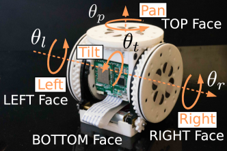
Figure 1: A SMORES-EP module has four active rotational degrees of freedom and four connectors using an array of electro-permanent (EP) magnets.

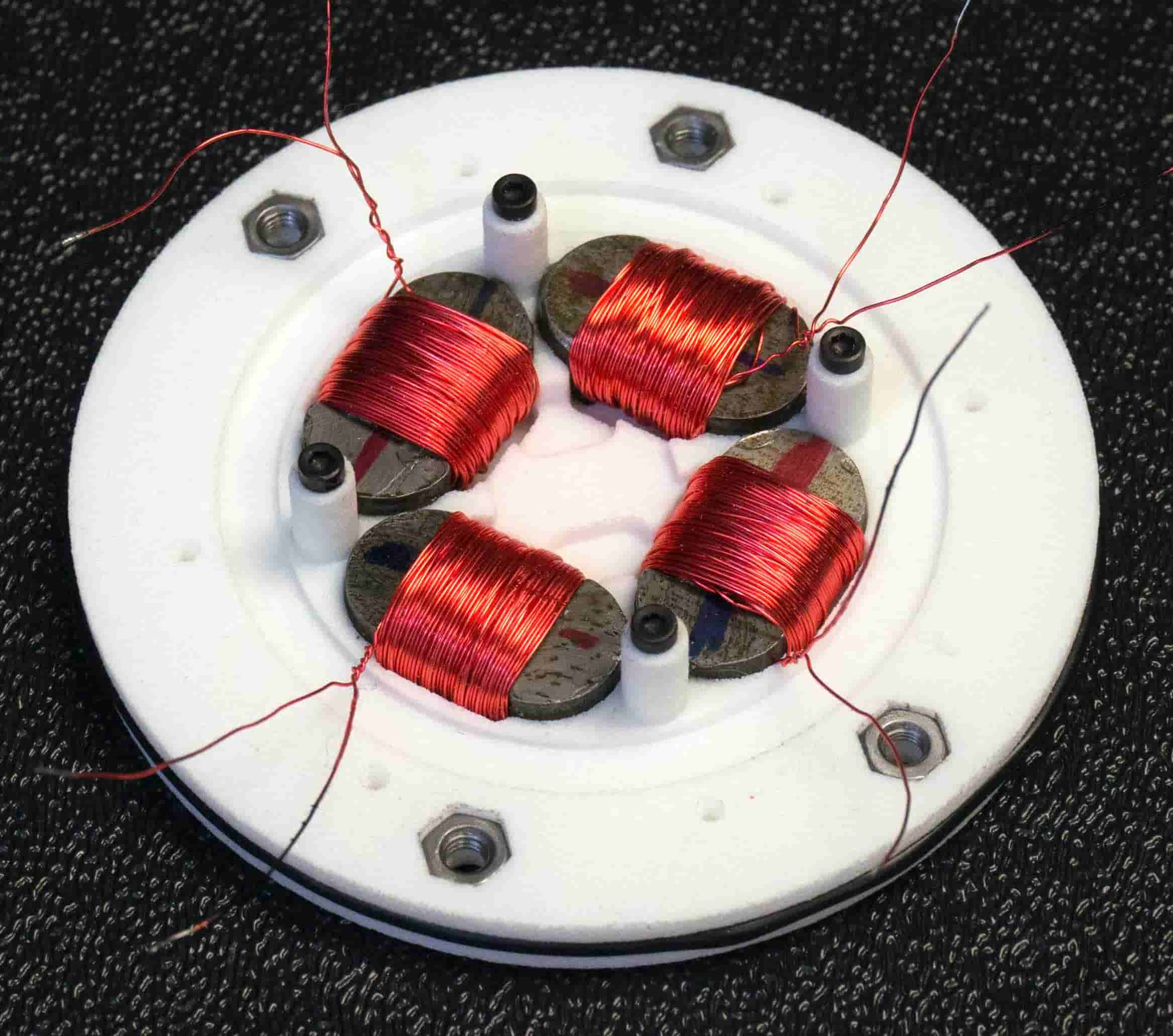
(a)

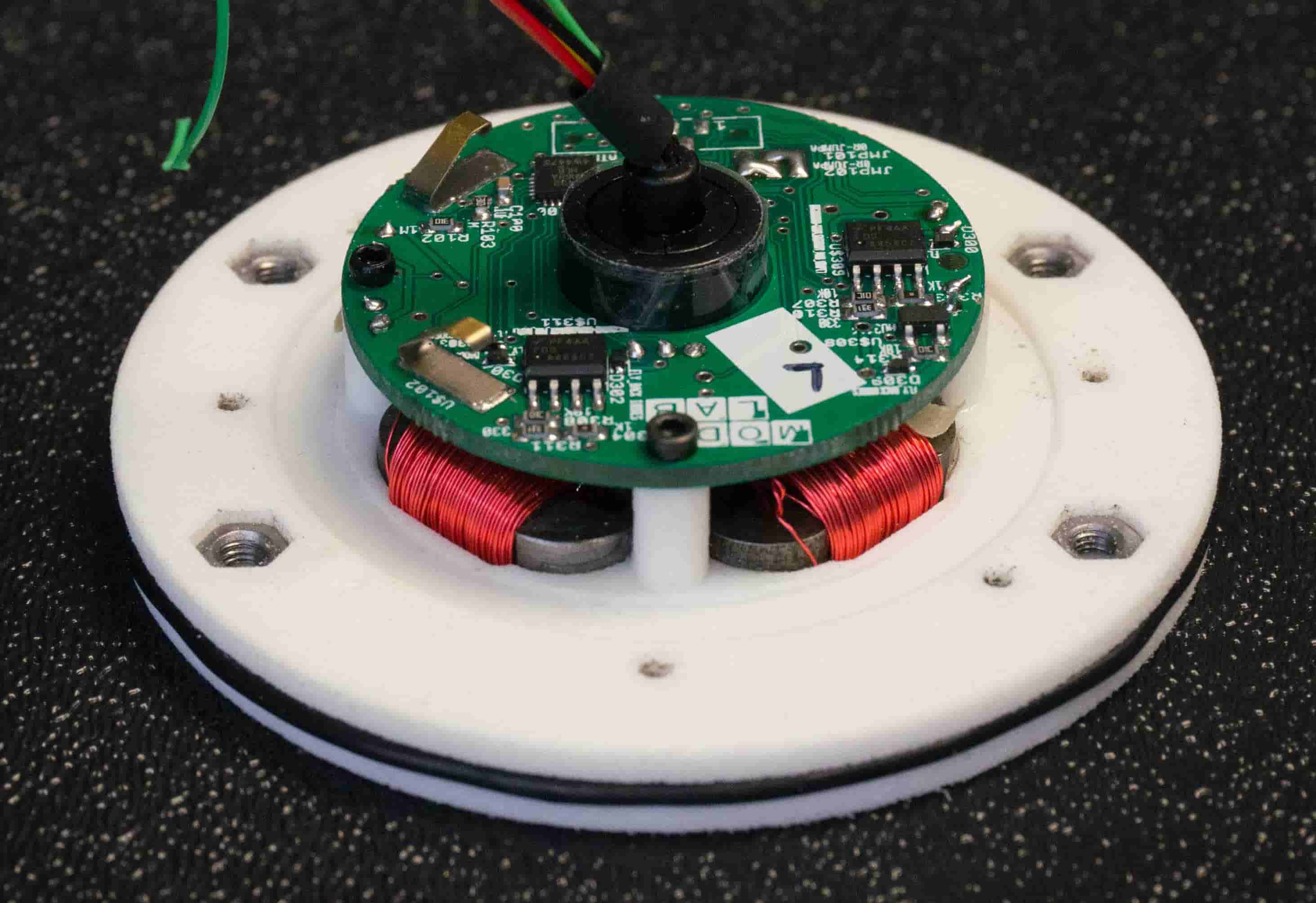
(b)

Figure 2: (a) Internal view of the magnets in the EP-Face. (b) Internal view of the EP-Face with circuit board.

The EP magnet is driven by three pulses under $11.1\text{\,}\mathrm{V}$ battery voltage. A pair of EP-Face connectors can provide as much as $90\text{\,}\mathrm{N}$ to maintain their docking status and very little energy is consumed to connect with or disconnect from each other. Magnetic forces can draw two modules together through a gap of $4\text{\,}\mathrm{m}\mathrm{m}$ normal, and $7\text{\,}\mathrm{m}\mathrm{m}$ parallel to the faces leading to a large area of acceptance.

Each module has an onboard processor, a Wi-Fi module, and a battery for hardware-level control and communication. This local processor handles all EP-Face connectors (generating pulses), all DOFs’ position estimation and control (running four Kalman filters at the same time), and the Wi-Fi communication with the central computer (UDP protocol). On the central computer, a robot manager is running for communication with all modules, including fetching information from an individual module, sending commands to control EP-Face connectors and motion of every DOF. Messages related to motion control are transmitted between the central computer and every module at around $40\text{\,}\mathrm{H}\mathrm{z}$ mainly for two purposes: (1) reporting the positions of all involved DOFs when executing manipulation tasks; (2) sending velocity commands of the left and right wheel when doing differential drive locomotion. This allows real-time control of a cluster of modules which is important to handle local scenarios that may cause collision among moving modules efficiently. All other information and commands, such as activating an EP-Face connector for docking and moving a DOF to a specific position, are transmitted as required by either programs or users.

In our experiment setup, we use a VICON motion capture system to localize module poses as they are moving on the ground. The system can provide precise pose estimation at $100\text{\,}\mathrm{H}\mathrm{z}$. This position data is used for the navigation of the modules moving as differential-drive vehicles.

4 Robot Configuration and Assembly

This section introduces a graph model to describe the topology of a modular robot system, the definition of our target topology, and the self-assembly problem.

4.1 Modular Robot Topology Configuration

A graph model of modular robot topology was presented by Liu and Yim (2017). A modular robot topology can be represented as a graph $G=(V,E)$ where $V$ is the set of vertices of $G$ representing all modules and $E$ is the set of edges of $G$ representing all the connections among modules. Graphs with only one path between each pair of vertices are trees. It is convenient to start with tree topology and, if a configuration has loops, it can be converted into an acyclic configuration by running a spanning tree algorithm. Therefore, this work only focuses on configurations in tree topology.

A tree $G=(V,E)$ can be rooted with respect to a vertex $\tau\in V$. Given a modular robot configuration in tree topology, the root is selected as the center of the graph defined by McColm (2004). Let $\mathcal{C}$ be the set of all connectors of a module that is $\{\mathrm{\textbf{L}},\mathrm{\textbf{R}},\mathrm{\textbf{T}},\mathrm{\textbf{B}}\}$, and $\mathrm{CN}^{v}(c)$ denotes the total number of modules connected to module $v$ via its connector $c\in\mathcal{C}$. Note that a configuration graph $G$ can be rooted with respect to any module but $\mathrm{CN}^{v}(c)$ is invariant under the selection of the root module. For any vertex $v\in V$ that is not a leaf with respect to root $\tau$, we denote its child connected via its connector $c$ as $\hat{v}^{c}$, the mating connector of $\hat{v}^{c}$ as $\hat{c}^{\prime}$, the set of its children as $\mathcal{N}(v,\tau)$, and the set of $c$ connected with its children as $\mathcal{C}_{d}(v)\subseteq\mathcal{C}$. Then the root module $\tau$ has to satisfy the following condition

$$\mathrm{CN}^{\tau}(c)\leq\frac{1}{2}|V|,\ \forall c\in\mathcal{C}$$ (1)

Input: Graph representation $G=(V,E)$

Output: Root module $\tau$

1 Root $G=(V,E)$ with respect to a module $v_{0}$ with height of $H$ and the height of $v\in V$ is $h(v)$;

2 Initialize $\mathrm{CN}^{v}(c)$ for $v\in V$ and $c\in\mathcal{C}$ to be zero;

3 Initialize $\mathbf{h}\leftarrow 1$;

4 while $\mathbf{h}\leq H$ do

5       foreach module $v$ with $h(v)=\mathbf{h}$ do

6             foreach module $\hat{v}^{c}\in\mathcal{N}(v,v_{0})$ do

7                   $\mathrm{CN}^{v}(c)\leftarrow\sum_{\hat{c}\in\mathcal{C}-\hat{c}^{\prime}}\mathrm{CN}^{\hat{v}^{c}}(\hat{c}),\ c\in\mathcal{C}_{d}(v)$;

8                   $\mathrm{CN}^{\hat{v}^{c}}(\hat{c}^{\prime})\leftarrow|V|-1-\sum_{\hat{c}\in\mathcal{C}_{d}(\hat{v})}\mathrm{CN}^{\hat{v}^{c}}(\hat{c})$;

9                  

10             end foreach

11            

12       end foreach

13      $\mathbf{h}\leftarrow\mathbf{h}+1$;

14 end while

$\tau\leftarrow v\in V$ such that $\mathrm{CN}^{\tau}(c)\leq\frac{1}{2}|V|$ $\forall c\in\mathcal{C}$

Algorithm 1 Root Module Search

A linear-time algorithm to compute the root of a modular robot configuration is shown in Algorithm 1. We first root the graph $G$ with respect to a randomly selected module $v_{0}$. Then the root module search can be formulated as a dynamic programming problem that can be solved in time $\mathcal{O}(|V|)$. The height of a vertex (module) $v$ in $G=(V,E)$ denoted as $h(v)$ is the number of the edges of the longest downward path to a leaf from $v$ and the height of a rooted graph is the height of its root. This bottom-up algorithm starts from vertices whose height are one. Detailed derivation can be found in the work by Liu and Yim (2017).

The depth of a vertex (module) $v$ in $G=(V,E)$ denoted as $d(v)$ can be defined as the number of the edges from $v$ to the root $\tau$. There are multiple ways to connect module $u$ and module $v$ denoted as $\mathrm{connect}(u,v)$ from module $u$’s point of view and $\mathrm{connect}(v,u)$ from module $v$’s point of view. Each connection has three attributes: Face, Face2Con, and Orientation (Liu and Yim, 2017). Some seemingly different connections are actually equivalent in topology. In a SMORES-EP configuration, attribute Orientation is trivial for the connections among LEFT Face, RIGHT Face, and TOP Face since the faces can rotate about the symmetry axis. However connections between two BOTTOM Faces cannot rotate, so Orientation mounted at $90\text{\,}\mathrm{\SIUnitSymbolDegree}$ increments (two of which are symmetric) needs to be considered (Orientation$\in\left[0,1\right]$) shown in Fig. 3.

(a)

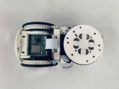
(b)

Figure 3: Connection between two BOTTOM Faces: (a) Orientation is 0 and (b) Orientation is 1.

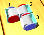
(a)

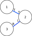
(b)

Figure 4: (a) A topology is built by three SMORES-EP modules. (b) The equivalent graph representation of the topology.

From here a SMORES-EP configuration can be fully defined. For example, a three-module configuration in a simulation environment (Tosun et al., 2018) is shown in Fig. 4a and its graph representation is shown in Fig. 4b. The connections in this topology can be written as:

$$\mathrm{connect}(1,2)= \{\mathrm{Face}:\mathrm{TOP\ Face},$$

$$\mathrm{Face2} \mathrm{Con}:\mathrm{TOP\ Face},\mathrm{Orientation}:\mathtt{Null}\}$$

$$\mathrm{connect}(2,1)= \{\mathrm{Face}:\mathrm{TOP\ Face},$$

$$\mathrm{Face2} \mathrm{Con}:\mathrm{TOP\ Face},\mathrm{Orientation}:\mathtt{Null}\}$$

$$\mathrm{connect}(2,3)= \{\mathrm{Face}:\mathrm{RIGHT\ Face},$$

$$\mathrm{Face2} \mathrm{Con}:\mathrm{LEFT\ Face},\mathrm{Orientation}:\mathtt{Null}\}$$

$$\mathrm{connect}(3,2)= \{\mathrm{Face}:\mathrm{LEFT\ Face},$$

$$\mathrm{Face2} \mathrm{Con}:\mathrm{RIGHT\ Face},\mathrm{Orientation}:\mathtt{Null}\}$$

In addition, for this simple topology, the root module is Module 2.

4.2 Self-assembly Problem

Assume there is a team of modules $\mathcal{M}=\{m_{1},m_{2},\cdots,m_{n}\}$ in the Euclidean space $\mathbb{R}^{2}$. The state of a module $m_{i}\in\mathcal{M}$ is defined as $p_{i}=\left[x_{i},y_{i},\theta_{i}\right]^{\intercal}$ where $o_{i}=\left[x_{i},y_{i}\right]^{\intercal}$ is the location of the center of $m_{i}$ and $\theta_{i}$ is the orientation of $m_{i}$. Then the distance between module $m_{i}$ and $m_{j}$ can be derived as $\|o_{i}-o_{j}\|$. Every SMORES-EP module is a cube with a side length of $w$. The assembly goal is a SMORES-EP tree topology configuration $G=(V,E)$ where $|V|=n$. Not all kinematic topology can be built by the self-assembly process. Only the kinematic topology that can be unfolded onto a plane can be achieved by a bunch of separated modules on the ground.

Definition 1

The target kinematic topology that can be self-assembled by separated modules is a modular robot configuration $G=(V,E)$ that can be fully unfolded to a plane satisfying:

1. $G$ is a connected graph;

2. The Euclidean distance between two adjacent modules is $w$;

3. The center of every module occupies a unique location.

Our target kinematic topologies are different from static assembled structures. For modular robots that are aiming for self-assembling static structures, the connections among the modules are homogeneous and the positions of the modules are enough to fully define the target. However, in our case, a module is composed of several joints and several modules can be connected in many ways to generate different kinematic chains. Hence, for our targets, we not only need to move the modules to their desired positions but also adjust their orientations to construct all connections defined in $E$ of $G$. We are not interested in all topologies that satisfy the constraints in Definition 1. Some topologies are less useful for executing tasks. For example, the connection in Fig. 3b shows the two BOTTOM Faces are connected with Orientation 1. This arrangement unnecessarily constrains the relative orientation between two modules so it is not considered in our work. In addition, the target topology is also meant to satisfy hardware constraints, such as the connector and the actuator limitations when lifting many modules.

The modules are at arbitrary locations with the constraint that the distance between any pair of modules $m_{i}$ and $m_{j}$ denoted as $d_{ij}$ is greater than $w$. The kinematic topology self-assembly problem is stated. Given a target kinematic topology $G=(V,E)$ and a team of $n$ modules $\mathcal{M}=\{m_{1},m_{2},\cdots,m_{n}\}$ where $n=|V|$, find a sequence of collision-free assembly actions to form the target kinematic topology.

5 Parallel Self-assembly Algorithm

We propose a parallel self-assembly algorithm for a set of modules to form a desired kinematic topology.

5.1 Task Assignment

In order to self-assemble $n$ separated modules into a target kinematic topology, we need to map the corresponding role of each module in the target. We model this problem as a task assignment problem, finding the optimal assignment solution among $n!$ different assignments with respect to some cost function.

Given a target kinematic topology $G=(V,E)$, first check if it satisfies the requirements in Definition 1 in order to be self-assembled and, if so, fully unfold it on the ground. Given the initial placement of all modules (in our case, all modules are placed on the ground with their electronics board facing upwards), the solution to unfold a kinematic topology is unique if the displacement of all modules remain unchanged. The root module $\tau$ of $G$ can be computed by Algorithm 1 in linear time. Then the state of each module $v_{i}\in V$ with respect to this root module $\tau$ denoted as $\bar{p}_{i}$ after fully unfolding $G$ can be computed in breadth-first search order starting from $\tau$. The state of a module is fully determined if the state of its parent module and the involved connection are known. For example, module $m_{i}$ is the parent of module $m_{j}$, with TOP Face of $m_{j}$ attached to TOP Face of $m_{i}$ shown in Fig. 5a (kinematic diagram in Fig. 5b). There are three more cases with TOP Face of $m_{i}$ being involved shown in Fig. 5c — Fig. 5e. In breadth-first search order, when visiting $m_{j}$, the state of $m_{i}$ with respect to $\tau$ should already be known that is $\bar{p}_{i}=\left[\bar{x}_{i},\bar{y}_{i},\bar{\theta}_{i}\right]^{\intercal}$. The state of $m_{j}$ with respect to $m_{i}$ denoted as $\bar{p}_{ji}$ is determined by the involved connectors, e.g., $\bar{p}_{ji}=\left[w,0,\pi\right]^{\intercal}$ for Fig. 5b. Then the state of $m_{j}$ with respect to $\tau$ is

$$\bar{p}_{j}=\left[\begin{array}[]{cc}R&0\\ 0&1\end{array}\right]\bar{p}_{ji}+\bar{p}_{i}$$ (2)

in which $R=\left[\begin{array}[]{cc}\cos\bar{\theta}_{i}&-\sin\bar{\theta}_{i}\\ \sin\bar{\theta}_{i}&\cos\bar{\theta}_{i}\end{array}\right]$.

(a)

(b)

(c)

(d)

(e)

Figure 5: (a) $m_{i}$ TOP Face is connected with $m_{j}$ TOP Face and (b) its kinematic diagram. (c) (d) (e) are the kinematic diagrams of three other cases when $m_{i}$ TOP Face is involved in the connection.

Given a set of $n$ modules $\mathcal{M}$, each $m\in\mathcal{M}$ needs to be mapped by a module $v\in V$ in an optimal way. In our task assignment problem, we want to minimize the total distance that all modules have to travel in order to assemble $G$. First, the center location of all modules can be defined as $o_{c}=\left[x_{c},y_{c}\right]^{\intercal}$ where $x_{c}=\sum_{i=1}^{n}x_{i}/n$ and $y_{c}=\sum_{i=1}^{n}y_{i}/n$. Then the root module is selected as

$$m_{\tau}=\underset{m_{i}\in\mathcal{M}}{\arg\min}\|o_{i}-o_{c}\|$$ (3)

The state of every module $m_{i}\in\mathcal{M}$ with respect to $m_{\tau}$ denoted as $\tilde{p}_{i}$ can be computed simply with a rigid body transformation. Obviously $\tilde{p}_{\tau}=\left[0,0,0\right]^{\intercal}$ that is the state of $m_{\tau}$ with respect to itself. Recall that $\bar{o}_{i}$ is the location of the center of $v_{i}$ with respect to $\tau\in V$. Given $m_{\tau}$ is mapped to $\tau$, namely $\|\tilde{o}_{\tau}-\bar{o}_{\tau}\|=0$, the distance between every pair of $m_{i}\in\mathcal{M}\setminus\{m_{\tau}\}$ and $v_{j}\in V\setminus\{\tau\}$ is simply $\|\tilde{o}_{i}-\bar{o}_{j}\|$ which is the cost of the task — moving to the location of $v_{j}$ — for module $m_{i}$. Other factors can also be included in the cost besides distance, such as the orientation. The optimal task assignment problem can be solved by Kuhn-Munkres algorithm or other concurrent assignment and planning of trajectories algorithms in polynomial time (Turpin et al., 2013). The output is a one-to-one and onto mapping $f:V\rightarrow\mathcal{M}$ which is used later by a motion planner to generate the assembly sequence.

5.2 Parallel Assembly Actions

With mapping $f:V\rightarrow\mathcal{M}$, we can compute the assembly sequence from the root to the leaves of $G$. In each step, the modules in $\mathcal{M}$ mapped to the modules in the target kinematic topology $G$ at the same depth can be executed in a parallel manner. Let $d(G)$ and $d(v)$ be the depth of the rooted graph $G$ and vertex $v\in V$ respectively, then for any vertex with $d(v)>0$, we denote its parent connected via its connector $c$ as $\tilde{v}^{c}$ and the mating connector of $\tilde{v}^{c}$ as $\tilde{c}^{\prime}$. An assembly action is a tuple of the form $(m_{i},c_{i},m_{j},c_{j})$ which means connect $m_{i}$’s connector $c_{i}$ with $m_{j}$’s connector $c_{j}$. The parallel assembly algorithm is shown in Algorithm 2. In every iteration, we first fetch all modules in the current depth from the target topology, then, with the optimal mapping $f:V\rightarrow\mathcal{M}$, the corresponding moving modules ($m$) are determined as well as their parent modules ($\tilde{m}^{c}$). We then have a group of assembly actions $A$ composed of $(m,c,\tilde{m}^{c},\tilde{c}^{\prime})$.

Input: Target Kinematic Topology $G=(V,E)$ with root $\tau$ and depth $d(G)$, $f:V\rightarrow\mathcal{M}$

Output: Parallel Assembly Sequence $\mathcal{A}$

1 $d\leftarrow 1$;

2 while $d\leq d(G)$ do

3       Create empty action queue $A$;

4       $\overline{V}\leftarrow\{v\in V|d(v)=d\}$;

5       for $v\in\overline{V}$ do

6             $m\leftarrow f(v)$;

7             $\tilde{m}^{c}\leftarrow f(\tilde{v}^{c})$;

8             $A.\mathrm{enqueue}((m,c,\tilde{m}^{c},\tilde{c}^{\prime}))$;

9            

10       end for

11      $\mathcal{A}.\mathrm{enqueue}(A)$;

12       $d\leftarrow d+1$;

13      

14 end while

Algorithm 2 Parallel Assembly

For each group of assembly actions $A\in\mathcal{A}$, all actions can be executed in parallel except when multiple modules are docking with different connectors of the root module. The group of assembly actions $A$ with the root module involved is separated into two subgroups: one group contains the actions for LEFT Face and RIGHT Face of the root module which can be executed first. The other group contains the actions for TOP Face and BOTTOM Face of the root module which are executed later. This is because the root module is not fixed to the ground and it is hard to ensure all modules to be attached can approach the root module simultaneously. When docking with a module that is not a root module, since this module is already attached to a group of modules, it is less likely to be pushed by other modules when executing the docking process. For each assembly action $a=(m_{i},c_{i},m_{j},c_{j})\in\mathcal{A}$, a motion controller first navigates $m_{i}$ to a location close to $m_{j}$ where the distance is determined by the grid size of the environment. Then module $m_{i}$ adjusts its pose to align the connector $c_{i}$ with $c_{j}$, and finally it approaches $c_{j}$ to finish the docking process. A square grid environment is generated once the root module is determined, with the root module at the center. The grid serves as a routing graph for navigating modules.

5.3 Docking Control

As mentioned, docking is a difficult part of self-assembly. We divide the docking process into three steps to ensure its success: navigation, pose adjustment, and approach.

5.3.1 Navigation

When doing self-assembly, each SMORES-EP module $m\in\mathcal{M}$ can behave as a differential-drive vehicle with the following kinematics model:

$$\dot{\tilde{p}}=\left[\begin{array}[]{c}\dot{\tilde{x}}\\ \dot{\tilde{y}}\\ \dot{\tilde{\theta}}\end{array}\right]=\left[\begin{array}[]{cc}\cos\tilde{\theta}&0\\ \sin\tilde{\theta}&0\\ 0&1\end{array}\right]\left[\begin{array}[]{c}v\\ \omega\end{array}\right]$$ (4)

in which $v$ is the linear velocity along $x$-axis of the body frame of $m_{i}$ and $\omega$ is the angular velocity around $z$-axis of body frame $m_{i}$ which are determined by the velocity of LEFT DOF and RIGHT DOF. Given a set of assembly actions $A\in\mathcal{A}$ in which all modules to be attached are at the same depth, the collision-free paths to navigate all involved modules can be generated by a multi-vehicle planner, e.g. Binder et al. (2019). Then, $\forall a=(m_{i},c_{i},m_{j},c_{j})\in A$, the module $m_{i}$ is controlled to follow a path to a location close to $m_{j}$ along the routes predefined by the grid environment. Every module is controlled by a real-time path-following controller and synchronized with other moving modules. Hence, prioritized planning approaches can be applied to handle potential collision among moving modules. For example, Binder et al. (2019) developed three simple strategies (Wait, Avoid, Push) combined with rescheduling method to handle possible local collision.

5.3.2 Pose Adjustment

Once the navigation procedure is done for all modules involved in $A\in\mathcal{A}$, $m_{i}$ starts to adjust its pose to align the involved connector. If $c_{i}$ (the connector of $m_{i}$ to be attached with $m_{j}$) is either LEFT Face or RIGHT Face, then adjust $x_{i}^{\prime}$ and $\theta_{i}^{\prime}$ to zeros where $x_{i}^{\prime}$ is the $x$ location of $m_{i}$ with respect to the body frame of $f^{-1}(m_{i})$ that is the goal pose of $m_{i}$ and $\theta_{i}^{\prime}$ is the orientation of $m_{i}$ with respect to the body frame of $f^{-1}(m_{i})$ (recall that $f$ is the mapping from $V\rightarrow\mathcal{M}$ derived by solving the task assignment problem). Otherwise, adjust $y_{i}^{\prime}$ and $\theta_{i}^{\prime}$ to zeros where $y_{i}^{\prime}$ is the $y$ location of $m_{i}$ with respect to the body frame of $f^{-1}(m_{i})$. Two cases are shown in Fig. 6. Note that this process has nothing to do with $c_{j}$. A kinematics model for the second case can be derived as

$$\left[\begin{array}[]{c}\dot{y}_{i}^{\prime}\\ \dot{\theta}_{i}^{\prime}\end{array}\right]=\left[\begin{array}[]{cc}\sin\theta_{i}^{\prime}&0\\ 0&1\end{array}\right]\left[\begin{array}[]{c}v\\ \omega\end{array}\right]$$ (5)

A control law to make $y_{i}^{\prime}$ and $\theta_{i}^{\prime}$ to converge to zeros is

$$\left[\begin{array}[]{c}v\\ \omega\end{array}\right]=\left[\begin{array}[]{cc}\sin\theta_{i}^{\prime}&0\\ 0&1\end{array}\right]^{-1}K_{2\times 2}\left[\begin{array}[]{c}-y_{i}^{\prime}\\ -\theta_{i}^{\prime}\end{array}\right]$$ (6)

where $K$ is positive definite and $K=\mathrm{diag}(2,1)$ in our experiments. A similar controller can be derived for the first case. For the pose adjustment controller, we relax the constraint on one dimension making the system fully actuated. For example, with the controller in Eq. (6), only $y_{i}^{\prime}$ and $\theta_{i}^{\prime}$ are under control and $x_{i}^{\prime}$ is no longer constrained, so $x_{i}^{\prime}$ may diverge possibly resulting in collision. However, this drift is not a concern for our modules which use differential drive with positioned controlled wheel motion. This is confirmed in our hardware experiments.

(a)

(b)

Figure 6: (a) The assembly action is to connect LEFT Face of $m_{i}$ with $m_{j}$ and $f^{-1}(m_{i})$ (the goal pose of $m_{i}$) is shown in dashed line. In this case, we have to align the connector by adjusting $x^{\prime}_{i}$ and $\theta^{\prime}_{i}$ to zeros. (b) If the assembly action is to connect TOP Face of $m_{i}$ with $m_{j}$, then we have to align the connector by adjusting $y^{\prime}_{i}$ and $\theta^{\prime}_{i}$ to zeros.

5.3.3 Approach

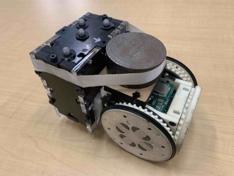
Figure 7: A helping module is a SMORES-EP module equipped with some payload so that it can lift another module.

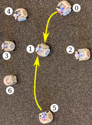
(a)

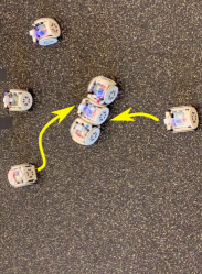
(b)

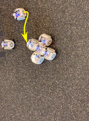
(c)

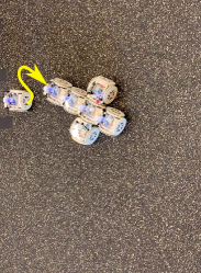
(d)

(e)

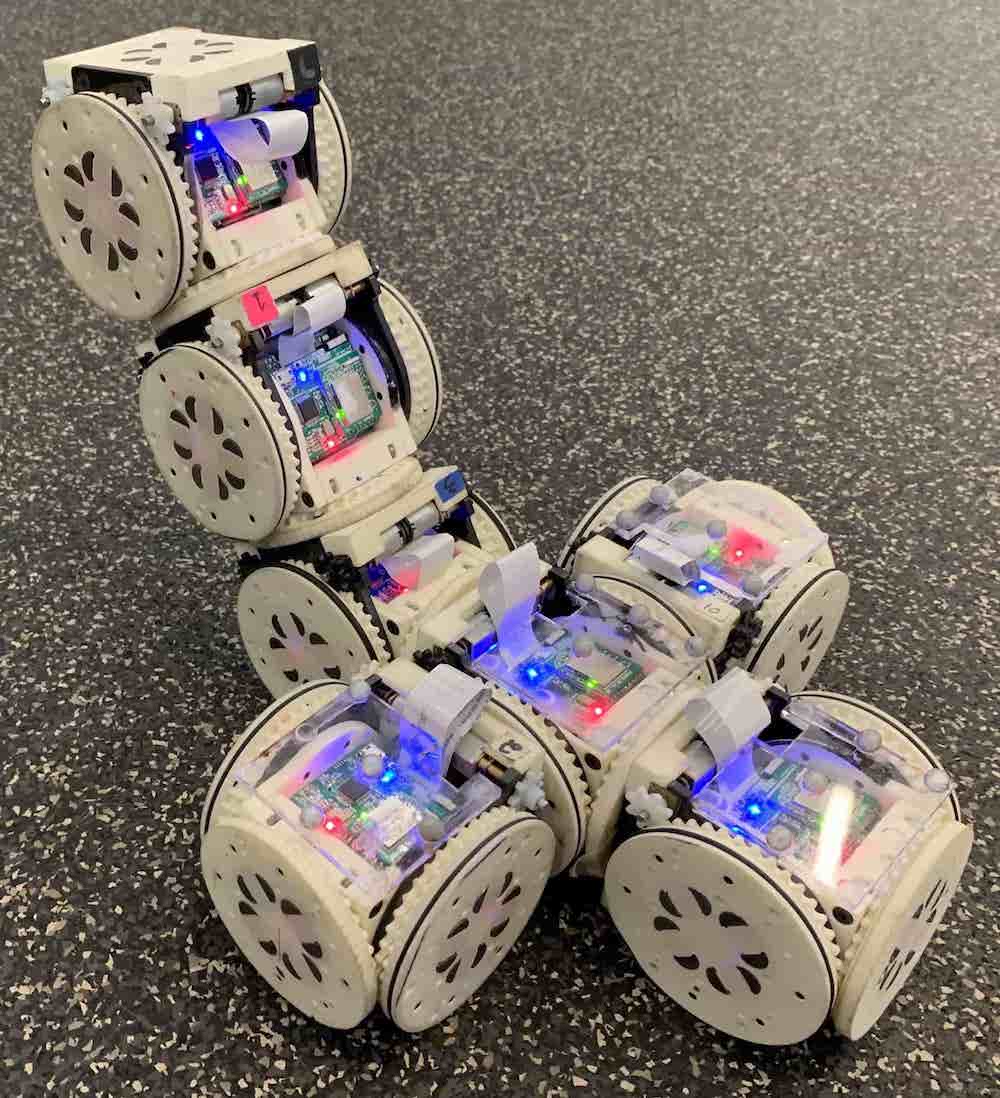
(f)

(g)

Figure 8: SMORES-EP hardware mobile manipulator self-assembly: (a) Execute actions $(0,\text{{B}},1,\text{{L}})$ and $(5,\text{{B}},1,\text{{R}})$; (b) Execute actions $(2,\text{{B}},1,\text{{T}})$ and $(6,\text{{T}},1,\text{{B}})$; (c) Execute action $(4,\text{{T}},6,\text{{B}})$; (d) Execute action $(3,\text{{T}},4,\text{{B}})$. (e) — (f) The final assembly. (g) The target kinematic topology.

The last step is to approach $c_{j}$ by moving in a straight line which is similar to the controller used in navigation step following a given trajectory. If $c_{i}$ is either TOP Face or BOTTOM Face, then module $m_{i}$ will first adjust $c_{i}$ to the right position and then keep moving pushing $m_{j}$ until $c_{i}$ and $c_{j}$ are fully connected. Otherwise, when $c_{i}$ is either LEFT Face or RIGHT Face, a helping module shown in Fig. 7 is needed. A new assembly action $(m_{\mathrm{H}},\text{{T}},m_{i},\bar{c}_{i})$ where $m_{\mathrm{H}}$ is a helping module and $\bar{c}_{i}$ is LEFT Face if $c_{i}$ is RIGHT Face, or the vice versa. After $m_{\mathrm{H}}$ is connected with $m_{i}$, $m_{i}$ is lifted so that it can adjust $c_{i}$ to the right position, delivered to its destination, and then placed down. Finally, $m_{\mathrm{H}}$ keeps moving to push $m_{i}$ to approach $m_{j}$ for docking. The helping module is a SMORES-EP module equipped with an extra mass on the BOTTOM Face as a counter balance while lifting a module. In our setup, there is only one helping module, and, for each assembly action group that is a queue, the helping module offers help sequentially. It is possible to have more to execute helping actions in parallel. While moving modules translate, the controller should keep the orientation of these modules fixed as docking requires the magnet faces to mate properly. To ease this requirement on the SMORES-EP modules the EP-Faces have a relatively large area of acceptance.

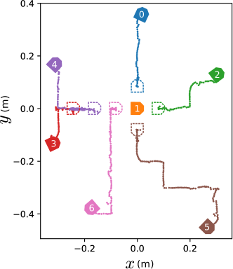
Figure 9: Actual path of each module for Task 1.

6 Experiments

Our framework and algorithm are demonstrated with SMORES-EP modules on three tasks to evaluate the hardware and software integration. All paths for modules are generated on an empty grid map where each grid cell is a square $10\text{\,}\mathrm{c}\mathrm{m}$$\times$$10\text{\,}\mathrm{c}\mathrm{m}$. We also show this framework can be used to speed up the self-reconfiguration process proposed by Liu et al. (2019).

Table 1: Initial Locations of All Modules in Task 1

Module	$x$ (m)	$y$ (m)	$\theta$ (rad)
Module 0	0.017	0.357	1.142
Module 1	0.0	0.0	0.0
Module 2	0.305	0.129	0.641
Module 3	-0.318	-0.132	0.454
Module 4	-0.318	0.158	0.823
Module 5	0.264	-0.448	-0.763
Module 6	-0.172	-0.380	-2.431

6.1 Task 1: Mobile Manipulator

The first task is to form a mobile vehicle with an arm that can reach higher locations as shown in Fig. 8g. There are seven modules involved with Module 1 selected as the root module $m_{\tau}$ which is closest to the center (Fig. 8a). The initial locations of all modules with respect to the root module is shown in Table 1. In the target topology (Fig. 8g), the root module $\tau$ is computed as Module 0. Hence Module 0 in the target topology $G=(V,E)$ is mapped to Module 1 in the set of modules $\mathcal{M}$ on the ground. The mapping $f:V\rightarrow\mathcal{M}$ that is $0\to 1$, $1\to 5$, $2\to 2$, $3\to 0$, $4\to 6$, $5\to 4$, and $6\to 3$ is then derived by Kuhn-Munkres algorithm.

The assembly sequence starts from all vertices $v\in V$ with depth of one in the target topology which include Module 0, Module 2, Module 5, and Module 6. Because the root module is involved in this step, the assembly actions are separated into two subgroups. Module 0 and Module 5 start moving first to dock with LEFT Face and RIGHT Face of Module 1 respectively (Fig. 8a), then Module 2 and Module 6 begin the docking process with TOP Face and BOTTOM Face of the root module (Fig. 8b). In this way, even Module 1 can be moved slightly after docking with Module 0 and Module 5, Module 2 and Module 6 can still dock with Module 1 successfully. Lastly, Module 4 and Module 3 execute the assembly actions (Fig. 8c and Fig. 8d). It takes 130 seconds to finish the whole assembly process with paths shown in Fig. 9. Two additional experiments in simulation with different initial settings are shown in Fig. 10.

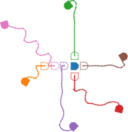
(a)

(b)

Figure 10: Two additional experiments for Task 1.

(a)

(b)

(c)

Figure 11: Adjustment of the position and orientation before executing assembly action $(3,\text{{T}},4,\text{{B}})$. (a) Module 3 finished navigation process and started to adjust its pose. (b) $y_{3}^{\prime}$ and $\theta_{3}^{\prime}$ have been adjusted and it started to approach the goal for docking. (c) The docking process of Module 3 was accomplished.

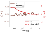
(a)

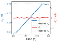
(b)

Figure 12: Pose adjustment of Module 3 before docking in Task 1: (a) adjusting $y_{3}^{\prime}$ and $\theta_{3}^{\prime}$; (b) adjusting $x_{3}^{\prime}$ while maintaining the correct orientation.

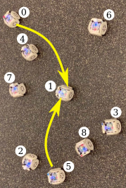
(a)

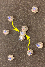
(b)

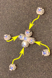
(c)

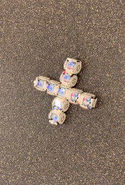
(d)

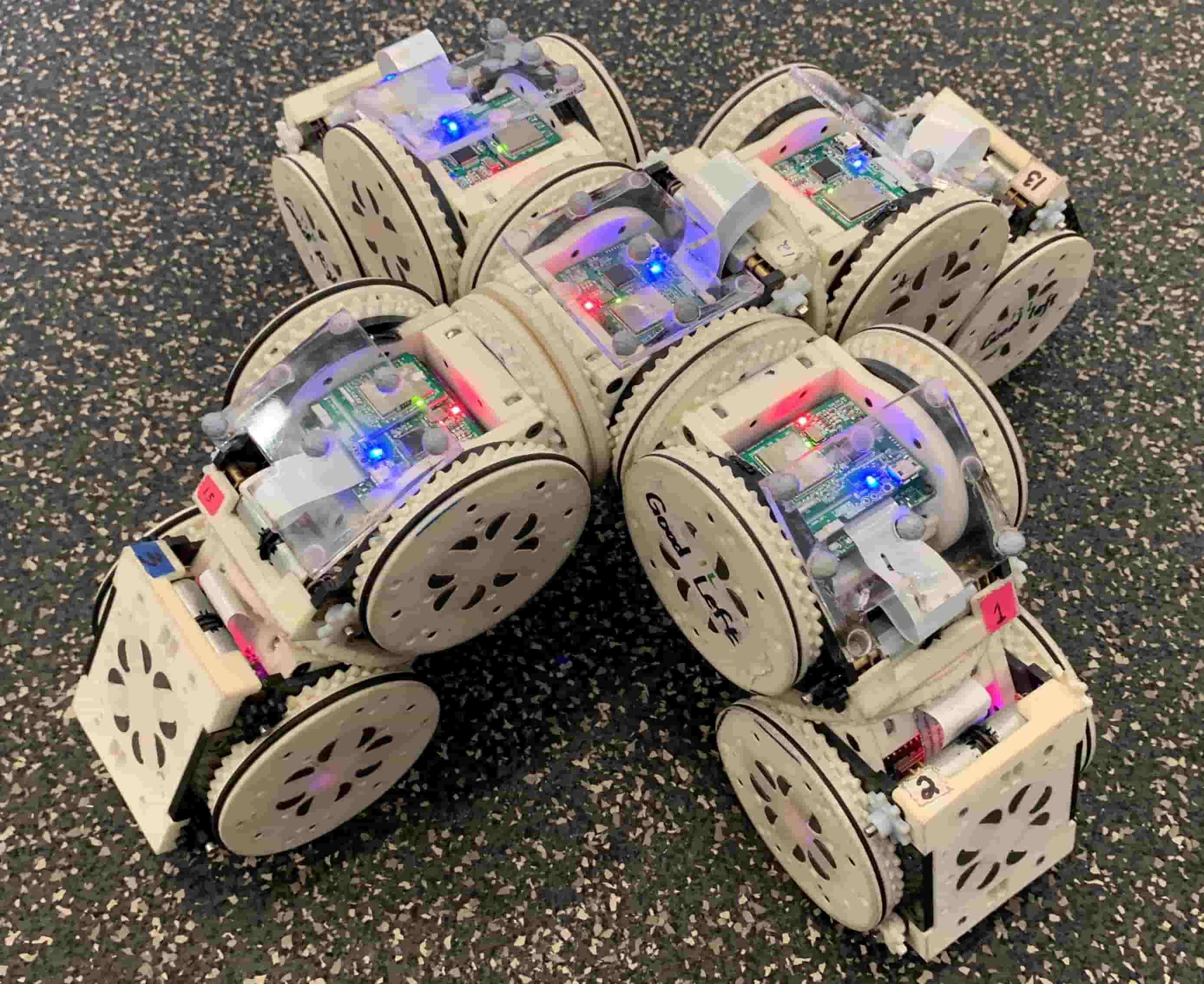
(e)

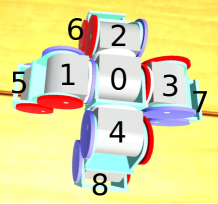
(f)

Figure 13: SMORES-EP hardware holonomic vehicle self-assembly: (a) Execute assembly actions $(0,\text{{T}},1,\text{{L}})$ and $(5,\text{{T}},1,\text{{R}})$; (b) Execute assembly actions $(4,\text{{T}},1,\text{{B}})$ and $(8,\text{{T}},1,\text{{T}})$; (c) Execute assembly actions $(3,\text{{T}},8,\text{{B}})$, $(2,\text{{T}},5,\text{{B}})$, $(7,\text{{T}},4,\text{{B}})$, and $(6,\text{{T}},0,\text{{B}})$. (d) — (e) The final assembly. (f) The target kinematic topology.

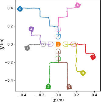
Figure 14: Actual path of each module for Task 2.

In a docking process, the controller for pose adjustment and approach ensures the success of docking. For example, for the last assembly action $(3,\text{{T}},4,\text{{B}})$, Module 3 first adjusts its body frame (Fig. 11a) so that its TOP Face is aligned with BOTTOM Face of Module 4 (Fig. 11b) and the performance is shown in Fig. 12a. The controller can adjust the pose of Module 3 quickly and align its connector within $6\text{\,}\mathrm{s}$ while almost keeping $x_{3}^{\prime}$ fixed. Then Module 3 moves forward to Module 4 for final docking (Fig. 11c) and the performance is shown in Fig. 12b. It can be seen that Module 3 can steadily approach Module 4 while maintaining its orientation fixed (very little oscillation of $\theta_{3}^{\prime}$ around zero value) so that the involved connector is always aligned.

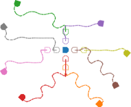
(a)

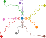
(b)

Figure 15: Two additional experiments for Task 2.

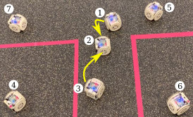
(a)

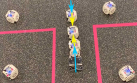
(b)

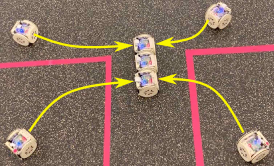
(c)

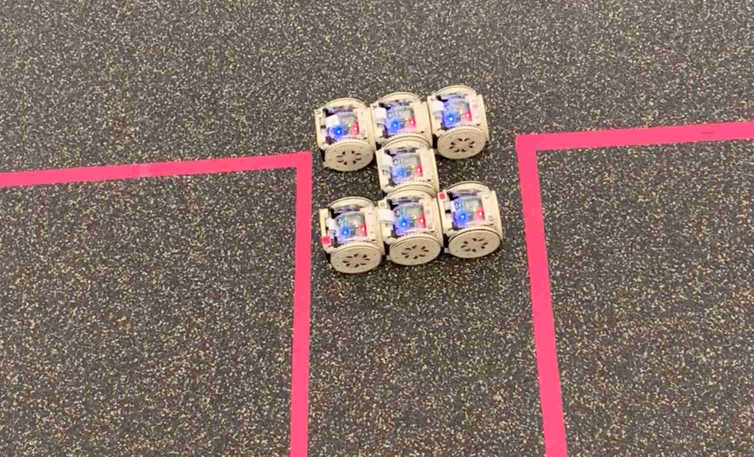
(d)

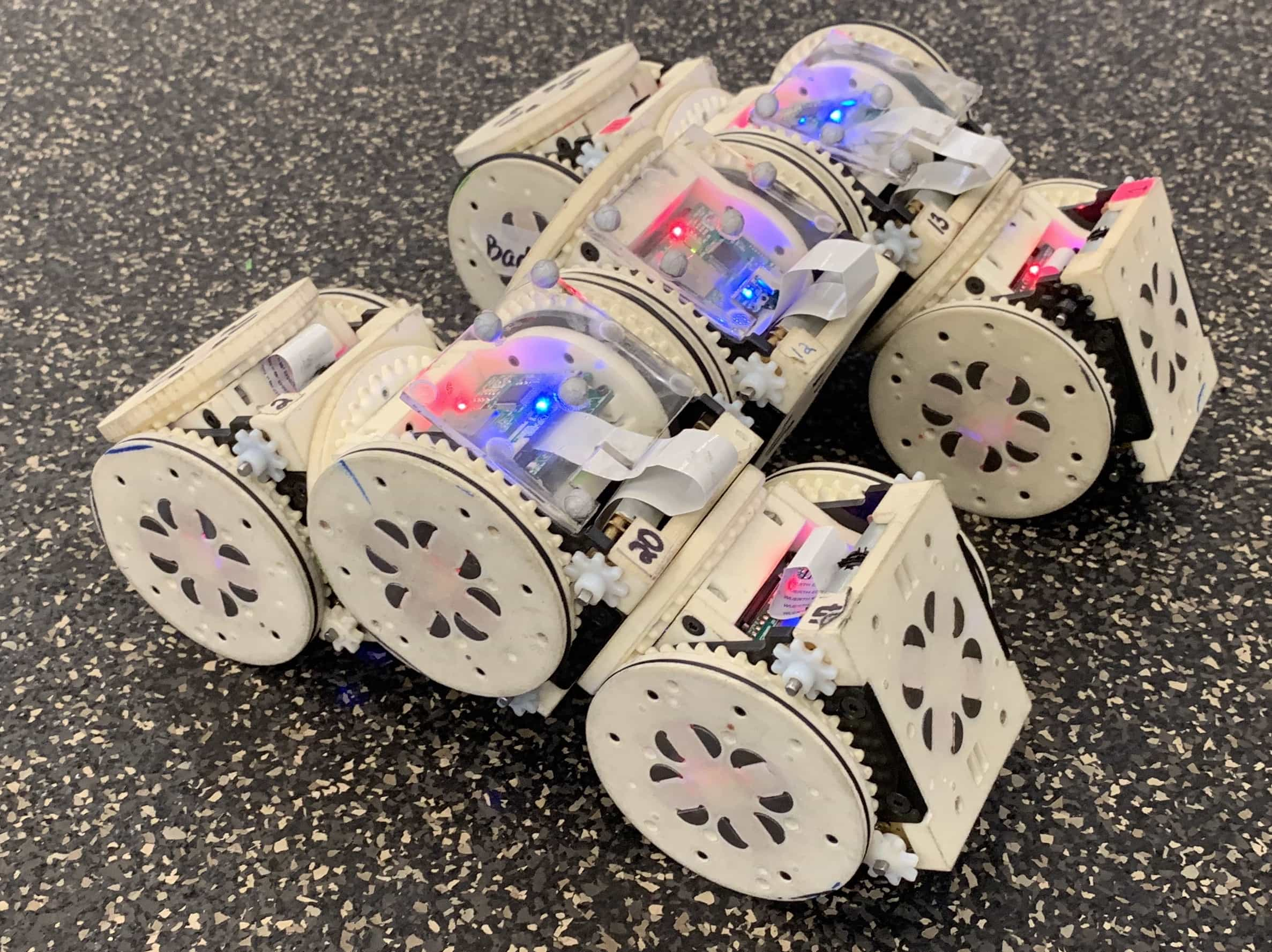
(e)

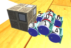
(f)

Figure 16: SMORES-EP hardware RC car self-assembly: (a) Execute actions $(1,\text{{R}},2,\text{{L}})$ and $(3,\text{{L}},2,\text{{R}})$; (b) A helping module is used to execute the current docking action; (c) Execute actions $(4,\text{{T}},3,\text{{B}})$, $(7,\text{{T}},1,\text{{B}})$, $(6,\text{{B}},3,\text{{T}})$, and $(5,\text{{B}},1,\text{{T}})$. (d) — (e) The final assembly. (f) The target kinematic topology.

6.2 Task 2: Holonomic Vehicle

Table 2: Initial Locations of All Modules in Task 2

Module	$x$(m)	$y$(m)	$\theta$(rad)
Module 0	-0.421	0.388	-0.760
Module 1	0.0	0.0	0.0
Module 2	-0.110	-0.469	1.445
Module 3	0.386	-0.143	0.509
Module 4	-0.343	0.082	-2.961
Module 5	0.118	-0.472	1.700
Module 6	0.215	0.428	-2.058
Module 7	-0.342	-0.044	-1.249
Module 8	0.270	-0.317	2.416

The second task assembles nine modules into a holonomic vehicle in order to move as in Fig. 13f. Based on the initial locations of all modules, the root module $m_{\tau}$ is then selected as Module 1. Then the pose of every module with respect to $m_{\tau}$ is computed and shown in Table 2. The root module of the target topology $G=(V,E)$ in Fig. 13f is Module 0. Given Module 0 in the target topology is mapped to Module 1 in this set of modules $\mathcal{M}$ on the ground, the optimal mapping $f:V\rightarrow\mathcal{M}$ is derived as $0\to 1$, $1\to 0$, $2\to 8$, $3\to 5$, $4\to 4$, $5\to 6$, $6\to 3$, $7\to 2$, and $8\to 7$. The assembly process is shown in Fig. 13a — Fig. 13c and the final assembly is shown in Fig. 13d and Fig. 13e. The behavior that the group of assembly actions is separated into two when root module is involved can be seen to ensure the success of the docking process. Then the rest of the assembly actions can be executed in parallel. Module 2, 3, 6, and 7 begin moving at the same time to locations close to their destinations, adjust their poses, and finally approach to execute docking actions. It takes 103 seconds in total to finish the whole assembly process. With our planner and controllers, the recorded actual path of every module in the experiment is illustrated in Fig. 14. Two additional experiments in simulation with different initial settings are shown in Fig. 15.

Table 3: Initial Locations of All Modules in Task 3

Module	$x$(m)	$y$(m)	$\theta$(rad)
Module 1	0.070	0.155	-1.352
Module 2	0.0	0.0	0.0
Module 3	-0.066	-0.250	0.997
Module 4	-0.299	0.170	0.811
Module 5	0.311	0.197	-2.539
Module 6	0.330	-0.373	-2.728
Module 7	-0.487	0.218	-0.436

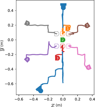
Figure 17: Actual path of each module in Task 3. The blue blocks without number labeled represent the helping modules.

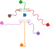
(a)

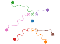
(b)

Figure 18: Two additional experiments for Task 3.

6.3 Task 3: RC Car

The last task assembles seven modules into a vehicle in order to push heavy items shown in Fig. 16f. The root module $m_{\tau}$ is selected as Module 2 that is the closest module to the center of the cluster. Then the initial locations of all modules with respect to $m_{\tau}$ are shown in Table 3. The root module $\tau$ of the target topology $G=(V,E)$ is Module 0, and given $m_{\tau}$ is mapped to $\tau$, the mapping $f:V\rightarrow\mathcal{M}$ that is $0\to 2$, $1\to 1$, $2\to 3$, $3\to 5$, $4\to 7$, $5\to 6$, and $6\to 4$ is derived. The assembly actions are shown in Fig. 16a — Fig. 16c. For the first step, we need to dock Module 1 RIGHT Face with Module 2 LEFT Face and dock Module 3 LEFT Face with Module 2 RIGHT Face. These two assembly actions cannot be executed directly since we cannot align the LEFT Face and RIGHT Face directly. We need the help of a helping module shown in Fig. 16b. In this experiment, there is only one helping module. Similar to common docking actions, the helping module first navigates to a location close to Module 3, then adjusts its pose to align its TOP Face, and approaches Module 3 RIGHT Face for docking. Then it lifts Module 3 so that Module 3 can adjust its LEFT Face. Finally the helping module delivers Module 3 to the desired location for docking with Module 2 RIGHT Face. This process repeats for Module 1 RIGHT Face. After both Module 1 and Module 3 are docked with the root module (Module 2), the rest of four modules can execute assembly actions in parallel. It takes 260 seconds in total to finish this assembly task, though 210 seconds are consumed by the helping module. More helping modules working in parallel would decrease the duration. The final assembly result is shown in Fig. 16d and Fig. 16e. The recorded path in the experiment is shown in Fig. 17. Two additional experiments in simulation with different initial settings are also shown in Fig. 18.

6.4 Reconfiguration Action Parallelization

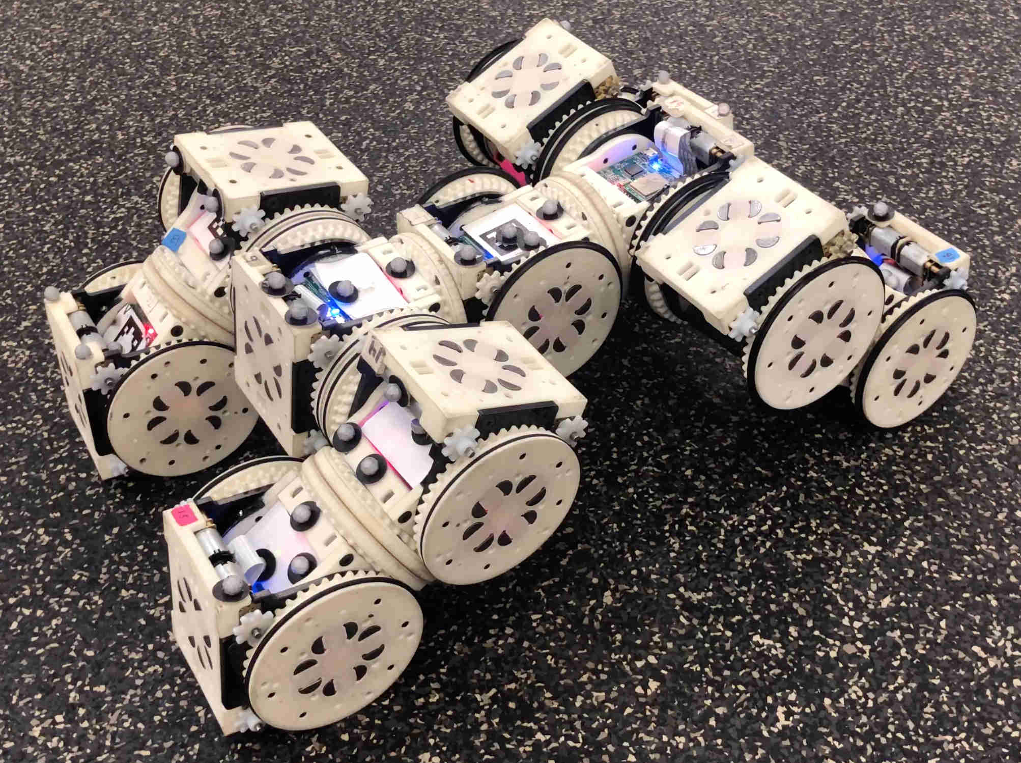
(a)

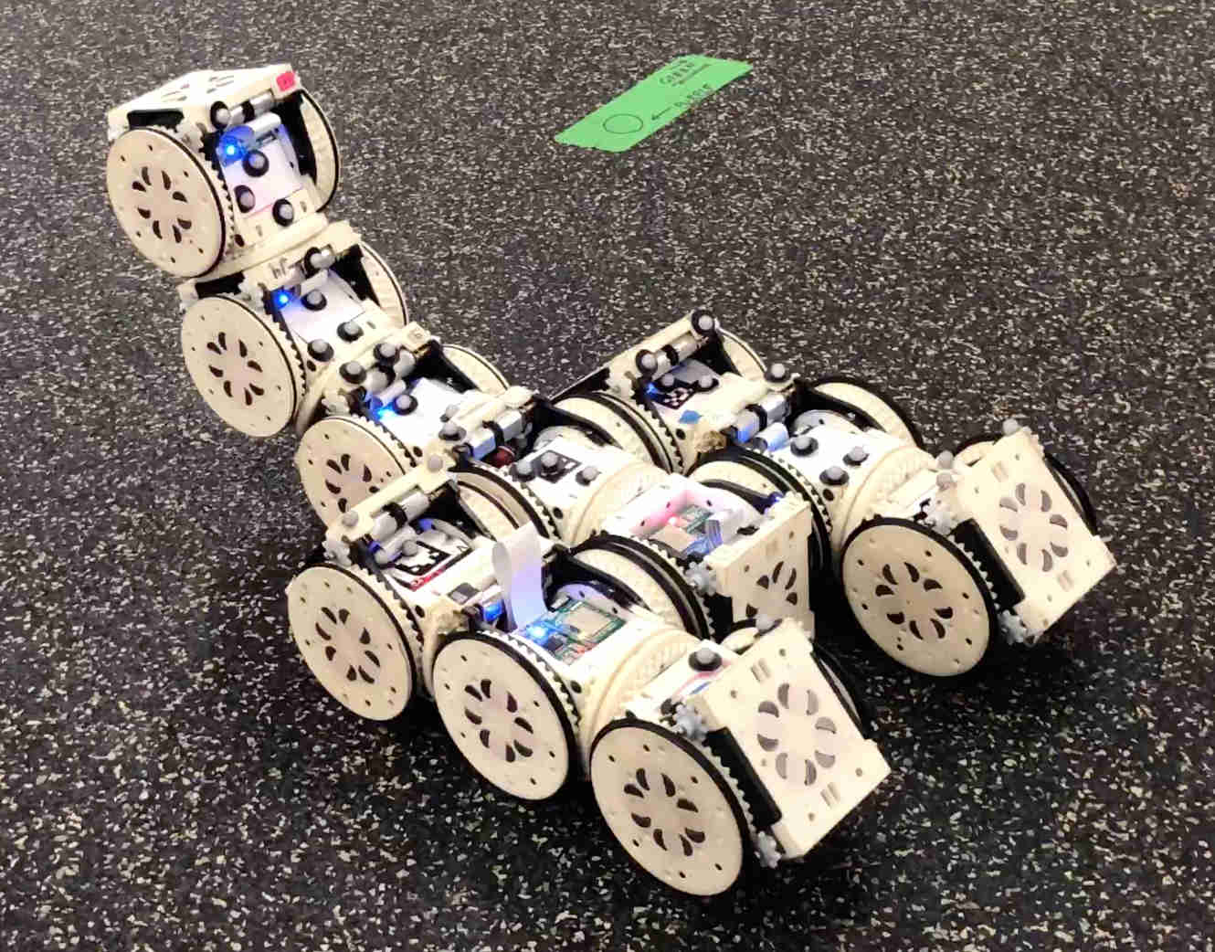
(b)

Figure 19: Reconfigure a walker configuration (a) into a mobile vehicle with an arm configuration (b) with eleven SMORES-EP modules involved.

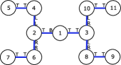
(a)

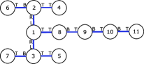
(b)

Figure 20: (a) The graph representation of the walker configuration. (b) The graph representation of the mobile manipulator configuration.

The algorithm by Liu et al. (2019) can output a sequence of reconfiguration actions which can be parallelized by our framework to speed up the process. These reconfiguration actions are executed from leaf modules to the root module. In addition to the docking action involved in a self-assembly action, a self-reconfiguration action also contains an undocking action beforehand. Given the initial configuration $G_{i}=(V_{i},E_{i})$ and goal configuration $G_{g}=(V_{g},E_{g})$, a mapping $f:V_{i}\rightarrow V_{g}$ as well as its inverse $f^{-1}:V_{g}\rightarrow V_{i}$ are computed, and each $v_{i}\in V_{i}$ is mapped to a unique $v_{g}\in V_{g}$, and $\tilde{v}_{i}^{c_{i}}$ and $\tilde{v}_{g}^{c_{g}}$ are their parents respectively. Then a sequence of reconfiguration actions can be generated. For example, given the task that is to reconfigure eleven SMORES-EP modules from a walker (Fig. 19a) into a mobile vehicle with an arm (Fig. 19b), their graph representations are shown in Fig. 20 where $\tau_{i}$ is Module 1 and $\tau_{g}$ is Module 1 respectively. The mapping $f:V_{i}\rightarrow V_{g}$ is computed as $1\to 1$, $3\to 8$, $9\to 5$, $8\to 3$, $2\to 9$, $11\to 4$, $10\to 2$, $4\to 6$, $6\to 10$, $5\to 7$, and $7\to 11$, and the corresponding reconfiguration actions are shown in Table 4.

Table 4: Reconfiguration Actions for Task 1

Action	ID	Face	ID	Face
Undock	5	TOP Face	4	TOP Face
Dock	5	TOP Face	8	BOTTOM Face
Undock	7	TOP Face	6	TOP Face
Dock	7	TOP Face	6	BOTTOM Face
Undock	4	LEFT Face	2	LEFT Face
Dock	4	TOP Face	10	BOTTOM Face
Undock	6	RIGHT Face	2	RIGHT Face
Dock	6	TOP Face	2	BOTTOM Face

As shown by Liu et al. (2019), these actions can be executed in sequential manner. This process can be parallelized by formulating all docking actions as a self-assembly problem. We first execute all undocking actions in Table 4 so that these modules are free to move. Then run the parallel algorithm (Algorithm 2) in which the target topology is the goal configuration, and the mapping is simply $f^{-1}:V_{g}\rightarrow V_{i}$ derived from the reconfiguration planner. The algorithm starts from modules in the goal configuration with depth being 1, but we ignore existing connections which are not constructed by docking actions in Table 4. By the mapping, the depth of Module 4 and Module 5 in the goal configuration are both 2, the depth of Module 6 is 3, and the depth of Module 7 is 4. Hence, the output of the assembly process is first $(5,\text{{T}},8,\text{{B}})$ and $(4,\text{{T}},10,\text{{B}})$ in parallel, then execute $(6,\text{{T}},2,\text{{B}})$, finally execute $(7,\text{{T}},6,\text{{B}})$. Some docking action may require other modules to move away to provide clearance as demonstrated by Liu et al. (2019). The strategy can also be used to handle self-assembly scenarios where modules are very close to each other.

7 Conclusion

In this paper, we present a parallel modular robot self-assembly framework for kinematic topology which can significantly improve the capability of modular robots to interact with the environment. SMORES-EP is a hybrid self-reconfigurable modular robot system. Each module has four DOFs and four EP-Face connectors in a compact space, and a swarm of modules are controlled by a hybrid architecture. Given a target kinematic topology, modules are mapped by those in the target configuration in an optimal way and then the assembly actions can be computed and executed in parallel. Motion controllers are developed to ensure the success of docking among modules. Hardware demonstrations show the effectiveness and robustness of the framework. This framework can also speed up the self-reconfiguration process by formulating all necessary docking actions as a self-assembly problem.

Future work includes creating demonstrations of arbitrary 3D structures with the SMORES-EP system. This is a capability which, in principle, should be possible with small changes to the algorithm, but is much harder to demonstrate using hardware with the concomitant complications of constraints from actuator limitations for lifting modules. Simulations with much larger structures would also demonstrate the scalability of this algorithm. Moreover, additional work needs to be done in order to move the system into the wild, including outdoor localization and wireless communication. The current hardware control architecture performs well but may encounter scalability issues when many more modules are involved. Hence exploring control structures that leverage different computation resources more efficiently is also important.