Radar Target Detection Aided by
Reconfigurable Intelligent Surfaces

Abstract

In this work, we consider the target detection problem in a sensing architecture where the radar is aided by a reconfigurable intelligent surface (RIS), that can be modeled as an array of sub-wavelength small reflective elements capable of imposing a tunable phase shift to the impinging waves and, ultimately, of providing the radar with an additional echo of the target. A theoretical analysis is carried out for closely- and widely-spaced (with respect to the target) radar and RIS and for different beampattern configurations, and some examples are provided to show that large gains can be achieved by the considered detection architecture.

I Introduction

One of the most striking technological innovations of the recent past in the field of radio communications is represented by metasurfaces [1], and in particular by reconfigurable intelligent surfaces (RISs) [2, 3, 4]. Traditionally, wireless communication and radar systems have been realized based on a proper design and optimization of the transmitter and of the receiver, assuming that no action could be taken to improve the channel propagation characteristics. This paradigm has been lately challenged by the introduction of RISs, which are man-made thin surfaces whose electromagnetic response can be electronically controlled. RISs are nearly passive devices, with very low energy consumption, which have the capability of tuning the phase, amplitude, frequency, and polarization of reflected impinging wavefronts [2]. As such, they introduce further degrees of freedom to be exploited for system optimization and allow shaping the wireless channel impulse response. They can be mounted outdoors on building facades or in indoor environments on the ceiling or on walls.

RISs have attracted a lot of interest in the recent past, and several studies have shown their usefulness for wireless communications. E.g., [5] has considered the downlink multiuser communication in a single-cell network with multiple antennas at the base station, and the RIS phase offsets have been optimized to increase the system energy efficiency; in [6], instead, the problem of massive access for IoT devices has been considered, and it is shown that the RIS provides remarkable gains to the system sum-rate. In [7], the authors have considered an indoor placement and have configured the RIS phases through a deep neural network. The use of a RIS in the context of millimeter-wave ultra massive MIMO systems has been investigated in [8]. Finally, the RIS-assisted localization has been investigated in [9, 10, 11].

All of these works have focused on the optimization of wireless communication systems, for either data exchange or localization (where the network is aware of the existence of a mobile device and can exploit the signals actively transmitted by the collaborating device). The possible benefits that a RIS could bring to a radar system in enhancing its detection capabilities are, to be best of the authors’ knowledge, a still unexplored topic, and this letter offers a first contribution aimed at filling this gap. We consider a scenario where the radar can transmit (or receive) through two separate beams, one pointing in the inspected direction and one pointing towards the RIS, which is aimed at focusing the impinging wavefront towards the prospective target during the transmission phase or towards the radar during the reception phase. In this framework, we provide key conditions for system design, that relate the signal bandwidth, the carrier frequency, and the sizes and mutual positions of radar, RIS, and prospective target; we inspect two relevant scenarios, where the radar and the RIS are closely- and widely-spaced, and we show that in both scenarios the RIS phases can be properly adjusted so as to align the echoes reaching the radar; we analyze two examples of realistic applications, and we show that the RIS can bring substantial improvements to the received signal-to-noise ratio (SNR); finally, we provide a detailed discussion, where we come up with relevant insights for system design, draw the conclusions, and outline future developments.

II System model

Consider a target detection problem where the radar is assisted by an RIS, as shown in Fig. 1, and denote by $P_{r}$ the radar transmit power, $\lambda$ the carrier wavelength, $L$ the number of sub-$\lambda$-sized surface element of the RIS, $\rho$, $d_{r,\ell}$ ($d_{r}$), and $d_{t,\ell}$ ($d_{t}$) the distances between the radar and the target, the $\ell$-th element (the center) of the RIS and the radar, and the $\ell$-th element (the center) of the RIS and the target, respectively, and $G_{rt}$ and $G_{rs,\ell}$ the gains of the radar beams towards the target and the $\ell$-th element of the RIS, respectively. We assume that the radar waveform is narrowband, so that the delays of the target echo reaching the elements of the RIS and of the target echo reaching the radar are not resolvable, i.e., $\max\{D_{rt},D_{rs},D_{s}\}\ll c/W$, where $D_{rt}$, $D_{rs}$, and $D_{s}$ are the size of the radar antenna pointing towards the target, of the radar antenna pointing towards the RIS, and of the RIS, respectively, $c$ is the speed of light, and $W$ is the radar signal bandwidth. Furthermore, we assume $\min\{D_{rt},D_{rs}\}\gg\lambda$, i.e., that the radar antennas are directive, and $D_{s}\gg\lambda$. Finally, we assume that the impinging wavefield can be approximated as a plane wave in the paths between radar and target, target and RIS, and radar and each element of the RIS; namely, we assume that the destinations in the aforementioned hops (in both directions) are in the far-field [12, 13], i.e.,

$$\begin{cases}\rho\geq 2\max\{D_{rt}^{2},D_{t}^{2}\}/\lambda\\ \min\{d_{t,\ell}\}_{\ell=1}^{L}\geq 2\max\{D_{t}^{2},D_{s}^{2}\}/\lambda\\ \min\{d_{r,\ell}\}_{\ell=1}^{L}\geq 2D_{rs}^{2}/\lambda\end{cases}$$ (1)

where $D_{t}$ is the size of the target. Observe that the whole RIS and the radar may not be in the far-field of each other.

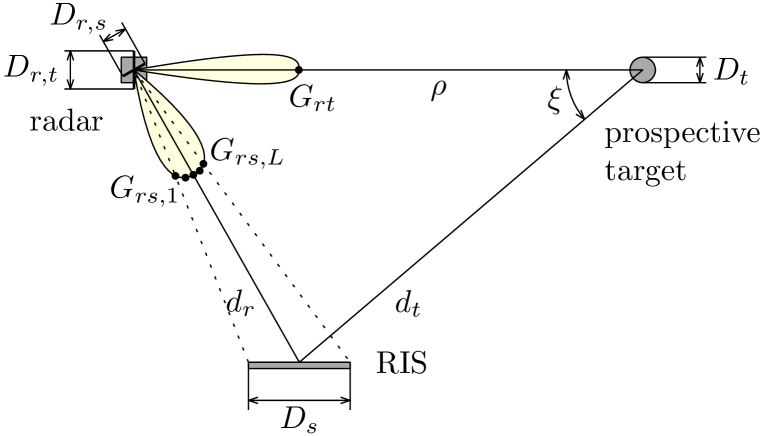
Figure 1: Considered architecture composed of a radar aided by an RIS.

In this framework, we analyze the following cases.

• Case a: the radar has one transmit beam pointing towards the target and two receive beams pointing towards the target and the RIS.

• Case b: the radar has two transmit beams pointing towards the target and the RIS and one receive beam pointing towards the target; the delays corresponding to the direct and indirect echoes are resolvable, namely, $d_{t}+d_{r}-\rho\geq c/W$.

• Case c: same as Case b, but the delays are not resolvable, i.e., $d_{t}+d_{r}-\rho\ll c/W$.

After matched-filtering with the transmit waveform and sampling, if a target is present in the resolution cell under test, the received discretized signal can be written as

$$\begin{pmatrix}x_{1}\\ x_{2}\end{pmatrix}=\begin{pmatrix}\alpha\sqrt{\sigma}\mathrm{e}^{\mathrm{i}\beta}\\ \sum_{\ell=1}^{L}\alpha_{sr,\ell}\sqrt{\sigma_{s}}\mathrm{e}^{\mathrm{i}(\psi_{t,\ell}+\phi_{\ell}+\psi_{r,\ell})}\end{pmatrix}+\begin{pmatrix}w_{1}\\ w_{2}\end{pmatrix}$$ (2a)

$$\begin{pmatrix}x_{1}\\ x_{2}\end{pmatrix}=\begin{pmatrix}\alpha\sqrt{\sigma\epsilon}\mathrm{e}^{\mathrm{i}\beta}\\ \sum_{\ell=1}^{L}\alpha_{st,\ell}\sqrt{\sigma_{s}(1-\epsilon)}\mathrm{e}^{\mathrm{i}(\psi_{r,\ell}+\phi_{\ell}+\psi_{t,\ell})}\end{pmatrix}+\begin{pmatrix}w_{1}\\ w_{2}\end{pmatrix}$$ (2b)

$$x_{1}=\alpha\sqrt{\sigma\epsilon}\mathrm{e}^{\mathrm{i}\beta}+\sum_{\ell=1}^{L}\alpha_{st,\ell}\sqrt{\sigma_{s}(1-\epsilon)}\mathrm{e}^{\mathrm{i}(\psi_{r,\ell}+\phi_{\ell}+\psi_{t,\ell})}+w_{1}$$ (2c)

for Case a, b, and c, respectively, where: $\sigma$ and $\sigma_{s}$ are the (unknown) target radar cross-sections (RCSs) observed from the radar and from the RIS, respectively; $\beta$ is the (unknown) phase of the radar-target channel; $\{\psi_{r,\ell}\}_{\ell=1}^{L}$ are the phases of the RIS-radar channel; $\{\phi_{\ell}\}_{\ell=1}^{L}$ are the (adjustable) RIS phases; $\{\psi_{t,\ell}\}_{\ell=1}^{L}$ are the (unknown) phases of the RIS-target channel; $w_{1}$ and $w_{2}$ are the noise components, modeled as independent and identically distributed complex circularly symmetric Gaussian random variables with variance $P_{w}$; $\epsilon\in[0,1]$ is the fraction of transmit power allocated to the direction of the target for Cases b and c; and, from the radar equation,

$$\alpha=\sqrt{\frac{P_{r}G_{rt}^{2}\lambda^{2}}{(4\pi)^{3}\rho^{4}}},\quad\alpha_{sr,\ell}=\sqrt{\frac{P_{r}G_{rt}G_{rs,\ell}\lambda^{2}S_{sr,\ell}}{(4\pi)^{4}\rho^{2}d_{t}^{2}d_{r,\ell}^{2}}}$$ (3)

$$\alpha_{st,\ell}=\sqrt{\frac{P_{r}G_{rt}G_{rs,\ell}\lambda^{2}S_{st,\ell}}{(4\pi)^{4}\rho^{2}d_{t}^{2}d_{r,\ell}^{2}}}$$ (4)

with $S_{sr,\ell}$ and $S_{st,\ell}$ denoting the (bistatic) RCSs of the $\ell$-th reflecting element of the RIS in the target-RIS-radar and radar-RIS-target paths, respectively.

The problem is to optimize the architecture in Fig. 1 so as to improve the detection performance of the radar by exploiting the additional target echo available from the RIS.

III System design

Depending on the size of the target, the antenna wavelength, and the mutual distances among radar, target, and RIS, we have two relevant situations. Namely, if $\xi\ll\lambda/D_{t}$, where $\xi$ is the angle formed by the line segment linking the target and the radar and the line segment linking the target and the RIS (cfr. Fig. 1), then radar and RIS are seen as closely-spaced (or co-located) by the target [15], since they lie in the same angular beam of the target scattering (that is proportional to $\lambda/D_{t}$). On the opposite extreme, we have the situation where radar and RIS are widely-spaced with respect to the target, i.e., $\xi\geq\lambda/D_{t}$. In the following, we address these two situations.

III-A Closely-spaced radar and RIS

In this case, we have that $\sigma_{s}=\sigma$ and $\psi_{t,\ell}=\psi_{t,\ell}^{\prime}+\beta$, for $\ell=1,\ldots,L$, where $\psi_{t,\ell}^{\prime}$ is known. Since $\psi_{r,\ell}$ can be estimated, the best performance is achieved when the RIS phases are chosen as $\phi_{\ell}=-\psi_{t,\ell}^{\prime}-\psi_{r,\ell}$, so that all the signal terms are phase-aligned, and (2) become

$$\begin{pmatrix}x_{1}\\ x_{2}\end{pmatrix} =\sqrt{\sigma}\mathrm{e}^{\mathrm{i}\beta}\begin{pmatrix}\alpha\\ \alpha_{sr}\end{pmatrix}+\begin{pmatrix}w_{1}\\ w_{2}\end{pmatrix}$$ (5a)

$$\begin{pmatrix}x_{1}\\ x_{2}\end{pmatrix} =\sqrt{\sigma}\mathrm{e}^{\mathrm{i}\beta}\begin{pmatrix}\alpha\sqrt{\epsilon}\\ \alpha_{st}\sqrt{1-\epsilon}\end{pmatrix}+\begin{pmatrix}w_{1}\\ w_{2}\end{pmatrix}$$ (5b)

$$x_{1} =\sqrt{\sigma}\mathrm{e}^{\mathrm{i}\beta}(\alpha\sqrt{\epsilon}+\alpha_{st}\sqrt{1-\epsilon})+w_{1}$$ (5c)

where $\alpha_{sr}=\sum_{\ell=1}^{L}\alpha_{sr,\ell}$ and $\alpha_{st}=\sum_{\ell=1}^{L}\alpha_{st,\ell}$. The generalized likelihood ratio tests (GLRTs) [16] with respect to the unknown complex parameter $\sqrt{\sigma}\mathrm{e}^{\mathrm{i}\beta}$ are

$$\begin{cases}\frac{\left|\alpha x_{1}+\alpha_{sr}x_{2}\right|^{2}}{(\alpha^{2}+\alpha_{sr}^{2})P_{w}}\gtrless\gamma,&\text{for Case\leavevmode\nobreak\ a}\\ \frac{\left|\alpha\sqrt{\epsilon}x_{1}+\alpha_{st}\sqrt{1-\epsilon}x_{2}\right|^{2}}{(\alpha^{2}\epsilon+\alpha_{st}^{2}(1-\epsilon))P_{w}}\gtrless\gamma,&\text{for Case\leavevmode\nobreak\ b}\\ \frac{|x_{1}|^{2}}{P_{w}}\gtrless\gamma,&\text{for Case\leavevmode\nobreak\ c}\end{cases}$$ (6)

where $\gamma>0$ is the detection threshold.

Denoting $\bar{\sigma}=\mathbbm{E}[\sigma]$, we have that the SNR is

$$\text{\sf SNR}_{a} =\frac{\bar{\sigma}(\alpha^{2}+\alpha_{sr}^{2})}{P_{w}}=\text{\sf SNR}_{0}(1+K_{sr})$$ (7a)

$$\text{\sf SNR}_{b} =\frac{\bar{\sigma}\alpha^{2}\epsilon+\alpha_{st}^{2}(1-\epsilon)}{P_{w}}\leq\text{\sf SNR}_{0}\max\{1,K_{st}\}$$ (7b)

$$\text{\sf SNR}_{c} =\frac{\bar{\sigma}(\alpha\sqrt{\epsilon}+\alpha_{st}\sqrt{1-\epsilon})^{2}}{P_{w}}\leq\text{\sf SNR}_{0}(1+K_{st})$$ (7c)

where $\text{\sf SNR}_{0}=\alpha^{2}\bar{\sigma}/P_{w}=P_{r}G_{rt}^{2}\lambda^{2}\bar{\sigma}/\bigl{(}(4\pi)^{3}\rho^{4}P_{w}\bigr{)}$ is the SNR when the RIS is absent, and

$$K_{sr} =\frac{\alpha_{sr}^{2}}{\alpha^{2}}=\frac{\rho^{2}}{4\pi d_{t}^{2}G_{rt}}\left(\sum_{\ell=1}^{L}\frac{\sqrt{G_{rs,\ell}S_{sr,\ell}}}{d_{r,\ell}}\right)^{2}$$ (8)

$$K_{st} =\frac{\alpha_{st}^{2}}{\alpha^{2}}=\frac{\rho^{2}}{4\pi d_{t}^{2}G_{rt}}\left(\sum_{\ell=1}^{L}\frac{\sqrt{G_{rs,\ell}S_{st,\ell}}}{d_{r,\ell}}\right)^{2}$$ (9)

are the power gains of the indirect echoes with respect to the direct one. Observe that the upper bounds on $\text{\sf SNR}_{b}$ and $\text{\sf SNR}_{c}$ are achieved by properly splitting the transmit power over the two available beams, i.e., by using $\epsilon_{b}^{*}=\mathbbm{1}_{\{K_{st}\leq 1\}}$, and $\epsilon_{c}^{*}=1/(1+K_{st})$, where $\mathbbm{1}_{\mathcal{A}}=1$, if the condition $\mathcal{A}$ holds true, and $\mathbbm{1}_{\mathcal{A}}=0$, otherwise.

The probability of false alarm is $P_{\text{fa}}=\mathrm{e}^{-\gamma}$, while the probability of detection, $P_{\text{d}}$, can be found once the distribution of $\sigma$ is given, and it admits the well-known, closed-form expressions for the Marcum’s non-fluctuating case and for the Swerling’s models [17].

III-B Widely-spaced radar and RIS

In this case, denoting $\beta_{s}=\psi_{t,1}$, we have that $\psi_{t,\ell}=\psi_{t,\ell}^{\prime\prime}+\beta_{s}$, where $\psi_{t,\ell}^{\prime\prime}$ is known. Again, the RIS phases can be chosen as $\phi_{\ell}=-\psi_{t,\ell}^{\prime\prime}-\psi_{r,\ell}$, so that (2) become

$$\begin{pmatrix}x_{1}\\ x_{2}\end{pmatrix} =\begin{pmatrix}\sqrt{\sigma}\mathrm{e}^{\mathrm{i}\beta}\alpha\\ \sqrt{\sigma_{s}}\mathrm{e}^{\mathrm{i}\beta_{s}}\alpha_{sr}\end{pmatrix}+\begin{pmatrix}w_{1}\\ w_{2}\end{pmatrix}$$ (10a)

$$\begin{pmatrix}x_{1}\\ x_{2}\end{pmatrix} =\begin{pmatrix}\sqrt{\sigma\epsilon}\mathrm{e}^{\mathrm{i}\beta}\alpha\\ \sqrt{\sigma_{s}(1-\epsilon)}\mathrm{e}^{\mathrm{i}\beta_{s}}\alpha_{st}\end{pmatrix}+\begin{pmatrix}w_{1}\\ w_{2}\end{pmatrix}$$ (10b)

$$x_{1} =\sqrt{\sigma\epsilon}\mathrm{e}^{\mathrm{i}\beta}\alpha+\sqrt{\sigma_{s}(1-\epsilon)}\mathrm{e}^{\mathrm{i}\beta_{s}}\alpha_{st}+w_{1}$$ (10c)

where $\sqrt{\sigma}\mathrm{e}^{\mathrm{i}\beta}$ and $\sqrt{\sigma_{s}}\mathrm{e}^{\mathrm{i}\beta_{s}}$ can be modeled as independent random variables, and the GLRTs are

$$\begin{cases}\frac{|x_{1}|^{2}+|x_{2}|^{2}}{P_{w}}\gtrless\gamma,&\text{for Cases\leavevmode\nobreak\ a and\leavevmode\nobreak\ b}\\ \frac{|x_{1}|^{2}}{P_{w}}\gtrless\gamma,&\text{for Case\leavevmode\nobreak\ c.}\end{cases}$$ (11)

Denoting $\bar{\sigma}_{s}=\mathbb{E}[\sigma_{s}]$, the SNRs for the two observations in Cases a and b are

$$\begin{cases}\text{\sf SNR}_{a,1}=\text{\sf SNR}_{0},\\ \text{\sf SNR}_{a,2}=\text{\sf SNR}_{0}K_{sr}\bar{\sigma}_{s}/\bar{\sigma},\end{cases}\begin{cases}\text{\sf SNR}_{b,1}=\epsilon\text{\sf SNR}_{0},\\ \text{\sf SNR}_{b,2}=(1-\epsilon)\text{\sf SNR}_{0}K_{st}\bar{\sigma}_{s}/\bar{\sigma}.\end{cases}$$ (12)

For Case c, assuming $\beta$ and $\beta_{s}$ uniformly distributed over $[0,2\pi)$, we have

$$\text{\sf SNR}_{c}=\bigl{(}\epsilon\bar{\sigma}\alpha^{2}+(1-\epsilon)\bar{\sigma}_{s}\alpha_{st}^{2}\bigr{)}/P_{w}.$$ (13)

Notice that $\epsilon$ in Cases b and c cannot be directly optimized, since the average RCSs of the target are in general unknown. If $\bar{\sigma}$ and $\bar{\sigma}_{s}$ are assumed to lie in $[\bar{\sigma}_{\text{min}},\bar{\sigma}_{\text{max}}]$ and $[\bar{\sigma}_{s,\text{min}},\bar{\sigma}_{s,\text{max}}]$, respectively, the choice that maximizes the worst-case $P_{d}$ is obtained for Case c by maximizing the worst-case SNR: specifically, we have $\epsilon_{c}^{*}=\mathbbm{1}_{\{K_{st}\bar{\sigma}_{s,\text{min}}/\bar{\sigma}_{\text{min}}\leq 1\}}$ that gives

$$\text{\sf SNR}_{c}\!=\!\text{\sf SNR}_{0}\bigl{(}\mathbbm{1}_{\{K_{st}\bar{\sigma}_{s,\text{min}}/\bar{\sigma}_{\text{min}}\leq 1\}}+\mathbbm{1}_{\{K_{st}\bar{\sigma}_{s,\text{min}}/\bar{\sigma}_{\text{min}}\geq 1\}}K_{st}\bar{\sigma}_{s}/\bar{\sigma}\bigr{)}.$$ (14)

For Case b, instead, $\epsilon_{b}^{*}$ depends on the target fluctuation model.

The probability of false alarm is $P_{\text{fa}}=\mathrm{e}^{-\gamma}(1+\gamma)$ for Cases a and b and $P_{fa}=\mathrm{e}^{-\gamma}$ for Case c [17], while, again, the probability of detection can be found once the distribution of $\sigma$ and $\sigma_{s}$ is given.

IV Examples

We consider a radar operating at 3 GHz equipped with two $1\times 1$ m uniform square arrays with a $\lambda/2$ element spacing and a cosine element pattern in both azimuth and elevation, and we examine two bandwidths, 1 and 10 MHz. The RIS is a square surface with inter-element spacing $\lambda/2$; the RCS of each element is modeled as $S_{sr,\ell}=S_{st,\ell}=\pi(\lambda/2)^{2}\cos\theta_{t}\cos\omega_{t}\cos\theta_{r,\ell}\cos\omega_{r,\ell}$, where $(\theta_{t},\omega_{t})$ and $(\theta_{r,\ell},\omega_{r,\ell})$ are the angles of incidence (azimuth, elevation) of the wave on the $\ell$-th element of the RIS from the target and the radar, respectively. The geometry of the system is depicted in Fig. 2, with the RIS parallel to the $x$-$z$ plane.

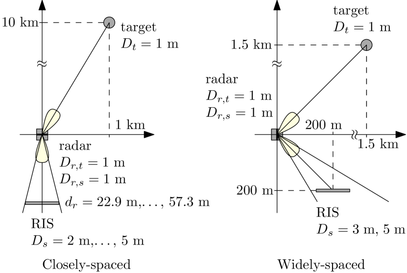
Figure 2: System geometry in the closely- and widely-spaced scenarios.

In the closely-spaced scenario, the radar antennas lie on the $x$-$z$ plane, and different RIS sizes are tested, ranging from 2 to 5 m; specifically, $d_{r}$ increases with the RIS size in such a way that the area covered by the 3-dB beamwidth of the radar antenna is equal to the RIS surface area. In the configuration with two transmit and one receive beam, Case b always holds when $W=10$ MHz, while Case c holds for $D_{s}\leq 3$ m when $W=1$ MHz. The SNR gain, measured by the ratio $\text{\sf SNR}_{a,b,c}/\text{\sf SNR}_{0}$, is reported in Table I: it is seen by inspection that a large performance improvement can be achieved in all operating conditions.

Table I: SNR gain [dB] in the closely-spaced scenario

$D_{s}$ [m]	2	2.5	3	3.5	4	4.5	5
$d_{r}$ [m]	22.9	28.6	34.4	40.1	45.8	51.5	57.3
Case a	4.78	6.17	7.41	8.53	9.54	10.5	11.3
Case b (10 MHz)	3.03	4.96	6.54	7.88	9.03	10.0	11.0
Case c (1 MHz)	4.78	6.17	7.41	—	—	—	—

In the widely-spaced scenario, the radar antennas lie on the $y$-$z$ plane, while the RIS has a side length of either 3 or 5 m. In the configuration with two transmit and one receive beam, Case b always holds for both bandwidths. An exponential fluctuation model is considered for the RCS of the target (a closed-form expression for $P_{d}$ is therefore available for all cases), and the parameter $\epsilon$ for Case b is selected so as to maximize the worst-case $P_{\text{d}}$ when $\bar{\sigma}_{s,\text{min}}=\bar{\sigma}_{\text{min}}$. Fig. 3 shows $P_{\text{d}}$ as a function of $\text{\sf SNR}_{0}$ when $P_{\text{fa}}=10^{-6}$ and $\bar{\sigma}_{s}=\bar{\sigma}$; the case without RIS has been included for the sake of comparison. It can be seen that a performance improvement is obtained with the RIS, and that Case a always outperforms Case b: indeed, since $K_{sr}=K_{st}$, the SNR’s in Case a are larger than those in Case b.

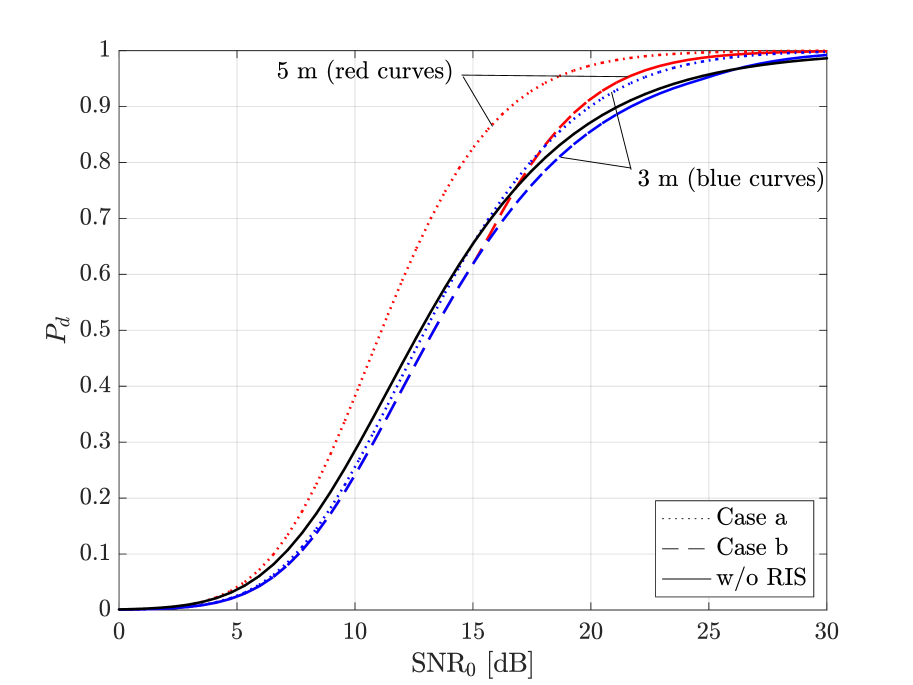
Figure 3: Probability of detection in the widely-spaced scenario; $P_{\text{fa}}=10^{-6}$.

V Discussion

Some useful insights on the performance improvement granted by the RIS can be gained, if the following approximations are made. Assume that $\theta_{r,\ell}\approx\theta_{r}$, $\omega_{r,\ell}\approx\omega_{r}$, $d_{r,\ell}\approx d_{r}$, and $G_{rs,\ell}\approx 4\pi d_{r}^{2}/A_{rs}$, where $A_{rs}$ is the surface area covered by the 3-dB beamwidth of the radar antenna at a distance equal to $d_{r}$, if the $\ell$-th element of the RIS falls in the 3-dB beamwidth, and $G_{rs,\ell}\approx 0$, otherwise. Let $A_{sr}=L(\lambda/2)^{2}\cos\theta_{r}\cos\omega_{r}$ be the effective area of the RIS seen from the radar, and $G_{st}=L\pi\cos\theta_{t}\cos\omega_{t}$ be the gain of the RIS (seen as an aperture antenna) towards the target. Then, $S_{st,\ell}=S_{sr,\ell}A_{sr}\approx G_{st}/L^{2}$, and

$$K_{sr}=K_{st}\approx\frac{\rho^{2}G_{st}}{d_{t}^{2}G_{rt}}\min\left\{\frac{A_{sr}}{A_{rs}},\frac{A_{rs}}{A_{sr}}\right\}$$ (15)

since the summation over $\ell$ encompasses about $L\min\{1,A_{rs}/A_{sr}\}$ terms. This shows that the RIS should be large and close enough so as to fill the area covered by the radar beam (as done in the closely-spaced example of Sec. IV), i.e., $A_{sr}\approx A_{rs}$: in this case, $K_{sr}=K_{st}\approx\rho^{2}G_{st}/(d_{t}^{2}G_{rt})$, which can be quite large for a small, low-cost radar and a large RIS. Basically, the radar beam pointing towards the RIS acts as a feed antenna, that sends/receives the signal via a large reconfigurable surface capable of electronically tunable beamforming. This can also be seen by noticing that the SNR corresponding to the indirect echo is

$$\frac{\bar{\sigma}\alpha_{st}^{2}}{P_{w}}=\frac{\bar{\sigma}\alpha_{sr}^{2}}{P_{w}}\approx\frac{P_{r}G_{rt}G_{st}\lambda^{2}\bar{\sigma}}{(4\pi)^{3}\rho^{2}d_{t}^{2}P_{w}}$$ (16)

that is just the radar equation, where the transmit or receive radar gain has been replaced by the RIS gain. If $G_{st}$ is much larger than $G_{rt}$, one may think to use only the beam pointing towards the RIS for both transmitting and receiving.

Finally, it is worthwhile noticing that, in the widely-spaced scenario, the proposed system realizes a low-cost bistatic radar, where a two-fold diversity is available in Cases a and b, thanks to the two observations with different aspect angles; this may also improve the estimation capabilities of the radar.

To conclude, the goal of this letter was to show that RISs can play a crucial role also in radar applications, and to unveil first fundamental trade-offs and main issues. Accordingly, a basic and simple setting was considered. Further research is needed to ascertain the beneficial effects of the RIS in more complex and challenging scenarios involving for instance the use of MIMO radars and of multiple distributed RISs, that can be simultaneously used in the transmit and receive phase.

On explicit request of one of the anonymous reviewers, we report here the detailed derivations of the main results and equations.

-A RIS-target channel phases in Footnote 4

Radar and RIS see the target from the same angle, and the phases of the target-RIS channel, $\{\psi_{t,\ell}\}_{\ell=1}^{L}$, can be expressed as $\psi_{t,\ell}^{\prime}+\beta$, where $\psi_{t,\ell}^{\prime}$ is known and depends only on the mutual position of the radar and the $\ell$-th element of the RIS with respect to the target, while $\beta$ is the phase of the target-radar channel, as it can also be seen from Fig. A1. In this case, we have the same radar cross-section (RCS) of the target, $\sqrt{\sigma}\mathrm{e}^{\mathrm{i}\beta}$, in both echoes.

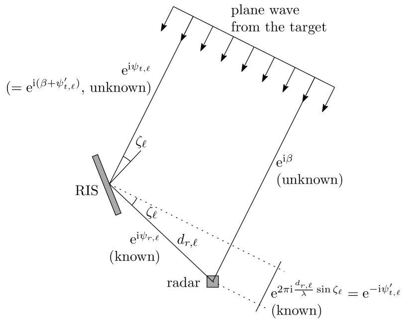
Figure A1: Phases of the RIS-target channel in the closely-spaced scenario.

-B GLRT’s in Eqs. (6)

The observation vector $\bm{x}=(x_{1}\;x_{2})^{\mathsf{T}}\in\mathbb{C}^{2}$ in Eq. (5a) is

$$\bm{x}=\sqrt{\sigma}\mathrm{e}^{\mathrm{i}\beta}\begin{pmatrix}\alpha\\ \alpha_{sr}\end{pmatrix}+\begin{pmatrix}w_{1}\\ w_{2}\end{pmatrix}=A\bm{\alpha}+\bm{w}$$ (A.17)

where $\bm{\alpha}=(\alpha\;\alpha_{sr})^{\mathsf{T}}\in\mathbb{R}^{2}$, $A=\sqrt{\sigma}\mathrm{e}^{\mathrm{i}\beta}\in\mathbb{C}$ is the target response, modeled as an unknown deterministic parameter, and $\bm{w}=(w_{1}\;w_{2})^{\mathsf{T}}\in\mathbb{C}^{2}$ is a complexy circularly symmetric Gaussian random vector with covariance matrix $P_{w}\bm{I}$. Therefore, the density of $\bm{x}$ is

$$\begin{cases}f_{1}(\bm{x};A)=\frac{1}{(\pi P_{w})^{2}}\mathrm{e}^{-\frac{1}{P_{w}}\|\bm{x}-A\bm{\alpha}\|^{2}},&\text{if the target is present}\\ f_{0}(\bm{x})=\frac{1}{(\pi P_{w})^{2}}\mathrm{e}^{-\frac{1}{P_{w}}\|\bm{x}\|^{2}},&\text{otherwise}\end{cases}$$ (A.18)

and the maximum likelihood (ML) estimate of $A$ under the “target presence” hypothesis is

$$\hat{A}_{\text{ML}} =\operatorname*{\arg\,\max}_{A\in\mathbb{C}}f_{1}(\bm{x};A)$$

$$=\operatorname*{\arg\,\min}_{A\in\mathbb{C}}\|\bm{x}-A\bm{\alpha}\|^{2}$$

$$=\frac{\bm{\alpha}^{\mathsf{T}}\bm{x}}{\|\bm{\alpha}\|^{2}}.$$ (A.19)

Thus, the GLRT is

$$\frac{f_{1}(\bm{x};\hat{A}_{\text{ML}})}{f_{0}(\bm{x})} =\mathrm{e}^{\frac{1}{P_{w}}\left(\|\bm{x}\|^{2}-\left\|\bm{x}-\frac{\bm{\alpha}^{\mathsf{T}}\bm{x}}{\|\bm{\alpha}\|^{2}}\bm{\alpha}\right\|^{2}\right)}$$

$$=\mathrm{e}^{\frac{|\bm{\alpha}^{\mathsf{T}}\bm{x}|^{2}}{\|\bm{\alpha}\|^{2}P_{w}}}\gtrless\gamma^{\prime}$$ (A.20)

i.e.,

$$\frac{|\bm{\alpha}^{\mathsf{T}}\bm{x}|^{2}}{\|\bm{\alpha}\|^{2}P_{w}}=\frac{|\alpha x_{1}+\alpha_{sr}x_{2}|^{2}}{(\alpha^{2}+\alpha_{sr}^{2})P_{w}}\gtrless\ln\gamma^{\prime}=\gamma$$ (A.21)

as shown is Eq. (6a). The other cases can similarly be handled.

-C SNRs in Eqs. (7)

The test statistic in Eq. (6), Case a, requires computing the quantity $\alpha x_{1}+\alpha_{sr}x_{2}=\bm{\alpha}^{\mathsf{T}}\bm{x}$. From Eq. (A.17) we have

$$\bm{\alpha}^{\mathsf{T}}\bm{x}=\bm{\alpha}^{\mathsf{T}}(A\bm{\alpha}+\bm{w})=A\|\bm{\alpha}\|^{2}+\bm{\alpha}^{\mathsf{T}}\bm{w}$$ (A.22)

so that

$$\text{\sf SNR}_{a}=\frac{\mathbb{E}[|A|]\|\bm{\alpha}\|^{4}}{\|\bm{\alpha}\|^{2}P_{w}}=\frac{\mathbb{E}[\sigma]\|\bm{\alpha}\|^{2}}{P_{w}}=\frac{\bar{\sigma}(\alpha^{2}+\alpha_{sr}^{2})}{P_{w}}$$ (A.23)

as reported in Eq. (7a). The other cases can similarly be handled. Finally, as to the maximization of $\text{\sf SNR}_{b}$ and $\text{\sf SNR}_{c}$ in Eqs. (7b) and (7c), we have

$$\max_{\epsilon\in[0,1]}\text{\sf SNR}_{b} =\max_{\epsilon\in[0,1]}\frac{\bar{\sigma}\alpha^{2}\epsilon+\alpha_{st}^{2}(1-\epsilon)}{P_{w}}$$

$$=\frac{\bar{\sigma}\max\{\alpha^{2},\alpha_{st}^{2}\}}{P_{w}}$$

$$=\frac{\bar{\sigma}\alpha^{2}}{P_{w}}\max\left\{1,\frac{\alpha_{st}^{2}}{\alpha^{2}}\right\}$$

$$=\text{\sf SNR}_{0}\max\{1,K_{st}\}$$ (A.24)

for $\epsilon=\epsilon^{*}_{b}=\mathbbm{1}_{\{\alpha^{2}_{st}\leq\alpha^{2}\}}=\mathbbm{1}_{\{K_{st}\leq 1\}}$, and

$$\max_{\epsilon\in[0,1]}\text{\sf SNR}_{b} =\max_{\epsilon\in[0,1]}\frac{\bar{\sigma}(\alpha\sqrt{\epsilon}+\alpha_{st}\sqrt{1-\epsilon})^{2}}{P_{w}}$$

$$=\frac{\bar{\sigma}\alpha^{2}+\alpha_{st}^{2}}{P_{w}}$$ (A.25)

$$=\frac{\bar{\sigma}\alpha^{2}}{P_{w}}\left(1+\frac{\alpha_{st}^{2}}{\alpha^{2}}\right)$$

$$=\text{\sf SNR}_{0}(1+K_{st})$$ (A.26)

for $\epsilon=\epsilon_{c}^{*}=\frac{\alpha^{2}}{\alpha^{2}+\alpha_{st}^{2}}=\frac{1}{1+K_{st}}$, respectively.

-D Detection probability in the closely-spaced scenario

Assuming $\sigma=\bar{\sigma}$ non fluctuating, $\sigma$ exponentially distributed with mean $\bar{\sigma}$, or $\sigma$ gamma distributed with mean $\bar{\sigma}$ and variance $\bar{\sigma}^{2}/2$, we have that the detection probability is

$$P_{\text{d}}=\begin{cases}Q\big{(}\sqrt{2\text{\sf SNR}},\sqrt{2\gamma}\big{)}&\text{(non fluctuating)}\\ \mathrm{e}^{-\frac{\gamma}{1+\text{\sf SNR}}}&\text{(exponential)}\\ \left(1+\frac{\gamma\frac{\text{\sf SNR}}{2}}{\left(1+\frac{\text{\sf SNR}}{2}\right)^{2}}\right)\mathrm{e}^{-\frac{\gamma}{1+\frac{\text{\sf SNR}}{2}}}&\text{(gamma)}\end{cases}$$ (A.27)

respectively, where SNR is as in Eqs. (7), and $Q(\,\cdot\,,\,\cdot\,)$ is the Marcum $Q$-function [16].

-E RIS-target channel phases in Footnote 5

Radar and RIS see the target from different aspect angles, and, since a plane wave is impinging on the RIS, the phases of the target-RIS channel can be expressed as $\psi_{t,\ell}^{\prime\prime}+\beta_{s}$, where $\beta_{s}$ is the phase of the channel between the target and the first element of the RIS, and $\psi_{t,\ell}^{\prime\prime}$ is known and depends only on the mutual position of the first and $\ell$-th element of the RIS with respect to the target; $\{\psi_{t,\ell}^{\prime\prime}\}_{\ell=1}^{L}$ are in fact the phases of a steering vector, as it can also be seen from Fig. A2. In this case, we have two different RCSs of the target, $\sqrt{\sigma}\mathrm{e}^{\mathrm{i}\beta}$ and $\sqrt{\sigma_{s}}\mathrm{e}^{\mathrm{i}\beta_{s}}$, in the two echoes, and they can be modeled as independent random variables.

Figure A2: Phases of the RIS-target channel in the widely-spaced scenario.

-F GLRT’s in Eqs. (11) and SNRs in Eqs. (12)

They can be proved as in the previous sections.

-G SNRs in Eqs. (13) and (14)

From Eq. (10c), the SNR in Case c is

$$\text{\sf SNR}_{c} =\frac{1}{P_{w}}\mathbb{E}\left[~\left|\sqrt{\sigma\epsilon}\mathrm{e}^{\mathrm{i}\beta}\alpha+\sqrt{\sigma_{s}(1-\epsilon)}\mathrm{e}^{\mathrm{i}\beta_{s}}\alpha_{st}\right|^{2}\right]$$

$$=\frac{1}{P_{w}}\Big{(}\mathbb{E}[\sigma]\alpha^{2}\epsilon+2\Re\left\{\mathbb{E}\left[\sqrt{\sigma}\mathrm{e}^{\mathrm{i}\beta}\sqrt{\sigma_{s}}\mathrm{e}^{-\mathrm{i}\beta_{s}}\right]\right\}$$

$$\quad\times\sqrt{\epsilon(1-\epsilon)}\alpha\alpha_{st}+\mathbb{E}[\sigma_{s}]\alpha_{st}^{2}(1-\epsilon)\Big{)}.$$ (A.28)

Since the two target responses, $\sqrt{\sigma}\mathrm{e}^{\mathrm{i}\beta}$ and $\sqrt{\sigma_{s}}\mathrm{e}^{\mathrm{i}\beta_{s}}$ are independent, and the phases $\beta$ and $\beta_{s}$ are uniformly distributed over $[0,2\pi)$, we have

$$\mathbb{E}\bigl{[}\sqrt{\sigma}\mathrm{e}^{\mathrm{i}\beta}\sqrt{\sigma_{s}}\mathrm{e}^{-\mathrm{i}\beta_{s}}\bigr{]}=\mathbb{E}\left[\sqrt{\sigma}\mathrm{e}^{\mathrm{i}\beta}\right]\mathbb{E}\left[\sqrt{\sigma_{s}}\mathrm{e}^{-\mathrm{i}\beta_{s}}\right]=0$$ (A.29)

and, therefore,

$$\text{\sf SNR}_{c} =\frac{\epsilon\bar{\sigma}\alpha^{2}+(1-\epsilon)\bar{\sigma}_{s}\alpha_{st}^{2}}{P_{w}}$$ (A.30)

as shown in Eq. (13). Concerning its optimization over $\epsilon\in[0,1]$, if $\bar{\sigma}\in[\bar{\sigma}_{\text{min}},\bar{\sigma}_{\text{max}}]$ and $\bar{\sigma}_{s}\in[\bar{\sigma}_{s,\text{min}},\bar{\sigma}_{s,\text{max}}]$, then the maximization of the worst-case SNR gives

$$\epsilon^{*}_{c} =\operatorname*{\arg\,\max}_{\epsilon\in[0,1]}\min_{\begin{subarray}{c}\bar{\sigma}\in[\bar{\sigma}_{\text{min}},\bar{\sigma}_{\text{max}}]\\ \bar{\sigma}_{s}\in[\bar{\sigma}_{\text{s,min}},\bar{\sigma}_{\text{s,max}}]\end{subarray}}\frac{\epsilon\bar{\sigma}\alpha^{2}+(1-\epsilon)\bar{\sigma}_{s}\alpha_{st}^{2}}{P_{w}}$$

$$=\operatorname*{\arg\,\max}_{\epsilon\in[0,1]}\frac{\epsilon\bar{\sigma}_{\text{min}}\alpha^{2}+(1-\epsilon)\bar{\sigma}_{s,\text{min}}\alpha_{st}^{2}}{P_{w}}$$

$$=\mathbbm{1}_{\{\bar{\sigma}_{s,\text{min}}\alpha^{2}_{st}\leq\bar{\sigma}_{\text{min}}\alpha^{2}\}}$$

$$=\mathbbm{1}_{\{K_{st}\bar{\sigma}_{s,\text{min}}/\bar{\sigma}_{\text{min}}\leq 1\}}$$ (A.31)

and this choice results in

$$\text{\sf SNR}_{c}\big{|}_{\epsilon=\epsilon_{c}^{*}} =\frac{\epsilon\bar{\sigma}\alpha^{2}+(1-\epsilon)\bar{\sigma}_{s}\alpha_{st}^{2}}{P_{w}}\Bigg{|}_{\epsilon=\epsilon_{c}^{*}}$$

$$=\begin{cases}\frac{\bar{\sigma}\alpha^{2}}{P_{w}}=\text{\sf SNR}_{0},\text{ if }K_{st}\bar{\sigma}_{s,\text{min}}/\bar{\sigma}_{\text{min}}\leq 1\\ \frac{\bar{\sigma}_{s}\alpha_{st}^{2}}{P_{w}}=\frac{\alpha_{st}^{2}}{\alpha^{2}}\frac{\bar{\sigma}_{s}}{\bar{\sigma}}\frac{\bar{\sigma}\alpha^{2}}{P_{w}}=K_{st}\frac{\bar{\sigma}_{s}}{\bar{\sigma}}\text{\sf SNR}_{0},\text{ otherwise}\end{cases}$$

$$=\text{\sf SNR}_{0}\Bigl{(}\mathbbm{1}_{\{K_{st}\bar{\sigma}_{s,\text{min}}/\bar{\sigma}_{\text{min}}\leq 1\}}$$

$$\quad+\mathbbm{1}_{\{K_{st}\bar{\sigma}_{s,\text{min}}/\bar{\sigma}_{\text{min}}\geq 1\}}K_{st}\frac{\bar{\sigma}_{s}}{\bar{\sigma}}\bigr{)}$$ (A.32)

as in Eq. (14).

-H Detection probability in the widely-spaced scenario

In Case c, the probability of detection is

$$P_{\text{d}}=\begin{cases}Q\big{(}\sqrt{2\text{\sf SNR}_{c}},\sqrt{2\gamma}\big{)}&\text{(non fluctuating)}\\ \mathrm{e}^{-\frac{\gamma}{1+\text{\sf SNR}_{c}}}&\text{(exponential)}\\ \left(1+\frac{\gamma\frac{\text{\sf SNR}_{c}}{2}}{\left(1+\frac{\text{\sf SNR}_{c}}{2}\right)^{2}}\right)\mathrm{e}^{-\frac{\gamma}{1+\frac{\text{\sf SNR}_{c}}{2}}}&\text{(gamma)}\end{cases}$$ (A.33)

respectively, where SNR is as in Eqs. (7). As to Cases a and b, $P_{\text{d}}$ does not admit a simple expression for these fluctuation models, since the SNRs of the two observations are in general different; for the exponential distribution, however, we have

$$P_{\text{d}}=\frac{1+\text{\sf SNR}_{2}}{\text{\sf SNR}_{1}-\text{\sf SNR}_{2}}\mathrm{e}^{-\frac{\gamma}{1+\text{\sf SNR}_{1}}}-\frac{1+\text{\sf SNR}_{1}}{\text{\sf SNR}_{1}-\text{\sf SNR}_{2}}\mathrm{e}^{-\frac{\gamma}{1+\text{\sf SNR}_{2}}}$$ (A.34)

where $\text{\sf SNR}_{1}$ and $\text{\sf SNR}_{2}$ are those in Eq. (12).

-I RIS gains in Eq. (15)

The approximations in Sec. V are

$$(\theta_{r,\ell},\omega_{r,\ell}) \approx(\theta_{r},\omega_{r})$$ (A.35a)

$$S_{sr,\ell} \approx\pi(\lambda/2)^{2}\cos\theta_{t}\cos\omega_{t}\cos\theta_{r}\cos\omega_{r}$$

$$=\frac{1}{L^{2}}\underbrace{L(\lambda/2)^{2}\cos\theta_{r}\cos\omega_{r}}_{A_{sr}}\underbrace{L\pi\cos\theta_{t}\cos\omega_{t}}_{G_{st}}$$

$$=\frac{A_{sr}G_{st}}{L^{2}}$$ (A.35b)

$$d_{r,\ell} \approx d_{r}$$ (A.35c)

$$G_{rs,\ell} \approx\frac{4\pi d_{r}^{2}}{A_{rs}}\mathbbm{1}_{\{\ell\in\mathcal{B}\}}$$ (A.35d)

where $A_{sr}$ is the effective area of the RIS seen from the radar, $G_{st}$ is the gain of the RIS (seen as an aperture antenna) towards the target, $A_{rs}$ is the surface area covered by the 3-dB beamwidth of the radar antenna at a distance equal to $d_{r}$, and $\mathcal{B}$ is the set containing the indexes of the elements of the RIS that fall in the 3-dB beamwidth of the radar. Therefore, the gain $K_{sr}$ in Eq. (8) can be approximated as

$$K_{sr} \approx\frac{\rho^{2}}{4\pi d_{t}^{2}G_{rt}}\left(\sum_{\ell=1}^{L}\sqrt{\frac{4\pi}{A_{rs}}\mathbbm{1}_{\{\ell\in\mathcal{B}\}}\frac{A_{sr}G_{st}}{L^{2}}}\right)^{2}$$

$$=\frac{\rho^{2}G_{st}}{d_{t}^{2}G_{rt}}\frac{A_{sr}}{A_{rs}}\frac{1}{L^{2}}\left(\sum_{\ell=1}^{L}\mathbbm{1}_{\{\ell\in\mathcal{B}\}}\right)^{2}$$

$$\approx\begin{cases}\frac{\rho^{2}G_{st}}{d_{t}^{2}G_{rt}}\frac{A_{sr}}{A_{rs}}\frac{1}{L^{2}}L^{2},&\text{if }A_{rs}\geq A_{sr}\\ \frac{\rho^{2}G_{st}}{d_{t}^{2}G_{rt}}\frac{A_{sr}}{A_{rs}}\frac{1}{L^{2}}\left(\frac{A_{rs}}{A_{sr}}\right)^{2},&\text{otherwise}\end{cases}$$

$$=\frac{\rho^{2}G_{st}}{d_{t}^{2}G_{rt}}\min\left\{\frac{A_{sr}}{A_{rs}},\frac{A_{rs}}{A_{sr}}\right\}$$ (A.36)

as in Eq. (15), where, in the third line, we have exploited the fact that $\sum_{\ell=1}^{L}\mathbbm{1}_{\{\ell\in\mathcal{B}\}}=L$, if the 3-dB beamwidth of the radar covers the entire RIS, i.e., if $A_{rs}\geq A_{sr}$, and $\sum_{\ell=1}^{L}\mathbbm{1}_{\{\ell\in\mathcal{B}\}}\approx A_{rs}/A_{sr}$, otherwise. The same approximation holds for $K_{st}$, since $S_{st,\ell}=S_{sr,\ell}$.

-J Radar Equation in (16)

Under the assumption that $A_{rs}\approx A_{sr}$ (i.e., that the area covered by the 3-dB beamwidth of the radar equals the effective area of the RIS seen from the radar), the SNR of the indirect echo in Cases b and c is, from Eqs. (3) and (15),

$$\frac{\bar{\sigma}\alpha_{st}^{2}}{P_{w}} =\frac{\bar{\sigma}\alpha^{2}}{P_{w}}\frac{\alpha_{st}^{2}}{\alpha^{2}}$$

$$=\frac{P_{r}G_{rt}^{2}\lambda^{2}\bar{\sigma}}{(4\pi)^{3}\rho^{4}P_{w}}K_{st}$$

$$\approx\frac{P_{r}G_{rt}^{2}\lambda^{2}\bar{\sigma}}{(4\pi)^{3}\rho^{4}P_{w}}\frac{\rho^{2}G_{st}}{d_{t}^{2}G_{rt}}$$

$$=\frac{P_{r}G_{rt}G_{st}\lambda^{2}\bar{\sigma}}{(4\pi)^{3}\rho^{2}d_{t}^{2}P_{w}}$$

as Eq. (16). The same approximation holds for the SNR of the indirect echo in Case a, $\bar{\sigma}\alpha_{sr}^{2}/P_{w}$, since $K_{sr}=K_{st}$.

References

• [1] O. Tsilipakos et al., “Toward intelligent metasurfaces: The progress from globally tunable metasurfaces to software-defined metasurfaces with an embedded network of controllers,” Adv. Opt. Mater., vol. 8, no. 17, p. 2000783, 2020.
• [2] E. Basar et al., “Wireless communications through reconfigurable intelligent surfaces,” IEEE Access, vol. 7, pp. 116 753–116 773, 2019.
• [3] Q. Wu and R. Zhang, “Towards smart and reconfigurable environment: Intelligent reflecting surface aided wireless network,” IEEE Commun. Mag., vol. 58, no. 1, pp. 106–112, 2019.
• [4] E. Björnson, O. Özdogan, and E. G. Larsson, “Reconfigurable intelligent surfaces: Three myths and two critical questions,” IEEE Commun. Mag., vol. 58, no. 12, pp. 90–96, 2020.
• [5] C. Huang, A. Zappone, G. C. Alexandropoulos, M. Debbah, and C. Yuen, “Reconfigurable intelligent surfaces for energy efficiency in wireless communication,” IEEE Trans. Wireless Commun., vol. 18, no. 8, pp. 4157–4170, 2019.
• [6] P. Mursia et al., “RISMA: Reconfigurable intelligent surfaces enabling beamforming for IoT massive access,” IEEE J. Sel. Areas Commun., vol. 39, no. 4, pp. 1072–1085, 2020.
• [7] C. Huang, G. C. Alexandropoulos, C. Yuen, and M. Debbah, “Indoor signal focusing with deep learning designed reconfigurable intelligent surfaces,” in IEEE Int. Workshop Signal Process. Adv. in Wireless Commun. (SPAWC), Jul. 2019.
• [8] V. Jamali, A. M. Tulino, G. Fischer, R. R. M uller, and R. Schober, “Intelligent surface-aided transmitter architectures for millimeter-wave ultra massive MIMO systems,” IEEE Open J. Commun. Soc., vol. 2, pp. 144–167, 2021.
• [9] H. Wymeersch, J. He, B. Denis, A. Clemente, and M. Juntti, “Radio localization and mapping with reconfigurable intelligent surfaces: Challenges, opportunities, and research directions,” IEEE Veh. Technol. Mag., vol. 15, no. 4, pp. 52–61, 2020.
• [10] J. He, H. Wymeersch, T. Sanguanpuak, O. Silven, and M. Juntti, “Adaptive beamforming design for mmwave RIS-aided joint localization and communication,” in IEEE Wireless Commun. Netw. Conf. Workshops (WCNCW), Apr. 2020, pp. 1–6.
• [11] A. Elzanaty, A. Guerra, F. Guidi, and M.-S. Alouini, “Reconfigurable intelligent surfaces for localization: Position and orientation error bounds,” arXiv preprint arXiv:2009.02818, 2020.
• [12] W. L. Stutzman and G. A. Thiele, Antenna Theory and Design, 2nd ed.   New York, NY, USA: John Wiley Sons, 1998.
• [13] C. A. Balanis, Advanced Engineering Electromagnetics, 2nd ed.   Hoboken, NJ, USA: Wiley, 2012.
• [14] M. I. Skolnik, Introduction to Radar Systems, 3rd ed.   New York, NY, USA: McGraw-Hill, 2001.
• [15] E. Fishler et al., “Spatial diversity in radars–models and detection performance,” IEEE Trans. Signal Process., vol. 54, no. 3, pp. 823–838, Mar. 2006.
• [16] H. L. Van Trees, Detection, estimation, and modulation theory.   New York, NY, USA: Wiley, 2001, vol. I: Detection, Estimation, and Linear Modulation Theory.
• [17] M. A. Richards, Fundamentals of radar signal processing.   New York, NY, USA: McGraw-Hill, 2005.
• [18] S. W. Ellingson, “Path loss in reconfigurable intelligent surface-enabled channels,” arXiv:1912.06759, 2019. [Online]. Available: http://arxiv.org/abs/1912.06759
• [19] W. Tang et al., “Wireless communications with reconfigurable intelligent surface: Path loss modeling and experimental measurement,” IEEE Trans. Wireless Commun., vol. 20, no. 1, pp. 421–439, Jan. 2021.