Sampling and Statistical Physics via Symmetry

Abstract

We formulate both Markov chain Monte Carlo (MCMC) sampling algorithms and basic statistical physics in terms of elementary symmetries. This perspective on sampling yields derivations of well-known MCMC algorithms and a new parallel algorithm that appears to converge more quickly than current state of the art methods. The symmetry perspective also yields a parsimonious framework for statistical physics and a practical approach to constructing meaningful notions of effective temperature and energy directly from time series data. We apply these latter ideas to Anosov systems.

1 Introduction

Sampling and statistical physics are essentially dual concepts. Phenomenologists sample from physical models to obtain data, and theorists construct physical models to explain data. For simple data and/or systems, the pushforward of an initial state distribution under a deterministic dynamical model may be theoretically adequate (at least up to a Lyapunov time or its ilk), but for complex data and/or systems, an intrinsically statistical model is typically necessary.

Moreover, sampling strategies and physical models are frequently manifestations of each other amey2018analysis . For instance, Glauber (spin-flip), Kawasaki (spin-exchange), and Swendsen-Wang (spin-cluster) dynamics are each both special-purpose Markov chain Monte Carlo (MCMC) algorithms and models for the time evolution of a spin system. Each algorithm/model has its own physical features, e.g. spin-flip dynamics are suited to the canonical ensemble; spin-exchange dynamics preserve an order parameter; and spin-cluster dynamics are both more efficient and descriptive for systems near criticality binder2019monte . As the chaotic hypothesis essentially stipulates that spin systems are generic statistical-physical systems gallavotti1995stationary ; gallavotti1999statistical , this blurring of the distinction between algorithm and model can also be regarded as generic.

Meanwhile, physics has a long tradition of formulating theories in terms of symmetries. Perhaps surprisingly, both sampling strategies and the basic structure of statistical physics itself can also be formulated in terms of symmetries. We outline these respective formulations with an eye towards (in §2) efficient parallel MCMC algorithms and (in §3) effective temperatures and energy functions that can be obtained directly from data for descriptive purposes. Finally, in §4 we apply the ideas of §3 to Anosov systems, where they suggest a broader framework for nonequilibrium statistical physics.

2 Sampling via symmetry

MCMC algorithms estimate expected values by running a Markov chain with the desired invariant measure. Though they arose from computational physics, MCMC algorithms have become ubiquitous, particularly in statistical inference and machine learning, and their importance in the toolkit of numerical algorithms is difficult to overstate richey2010mcmc ; brooks2011mcmc .

As such, there is a vast literature on MCMC algorithms. However, there is also much still left unexplored. As we shall see, the interface between MCMC algorithms and the theory of Lie groups and Lie algebras holds a surprise. A key observation is that the space of transition matrices with a given invariant measure is a monoid that is closely related to a Lie group. Certain natural elements of this monoid with simple closed form expressions naturally lead to constructions of the classical Barker and Metropolis MCMC samplers. These constructions generalize, leading to higher-order versions of samplers that respectively correspond to the ensemble MCMC algorithm of neal2011ensemble and an algorithm of delmas2009does . A further generalization leads to a new algorithm that we call the higher-order programming solver and whose convergence appears to improve on the state of the art. Each of these algorithms is only presently defined for finite state spaces and leaves the proposal mechanism unspecified: indeed, our entire focus is on acceptance mechanisms.

In this section, which is based on the conference paper huntsman2020fast , we review the basics of MCMC, Lie theory, and related work in §2.1. We then briefly consider the Lie group generated by a probability measure in §2.2. In particular, we construct a convenient basis of the subalgebra of the stochastic Lie algebra that annihilates a target probability measure $p$. This basis only requires knowledge of $p$ up to a multiplicative factor (e.g., a partition function), and this fact is the essential reason why MCMC algorithms work in general. In §2.3, we show how we can analytically produce transition matrices that leave $p$ invariant. We then construct the Barker and Metropolis samplers from Lie-theoretic considerations in §2.4. In §2.5, we extend earlier results, leading to generalizations of the Barker and Metropolis samplers that entertain multiple proposals at once and that we explicitly construct in §2.6. We then demonstrate the behavior of these samplers on a small spin glass in §2.7. In §2.8, we outline the construction of multiple-proposal transition matrices that are closest in Frobenius norm to the “ideal” transition matrix $1p$, and we introduce and demonstrate the resulting higher-order programming solver. Finally, we close our discussion of MCMC algorithms with remarks in §2.9.

2.1 Background

Markov chain Monte Carlo

As we have already mentioned in §2 and (e.g.) bremaud1999markov discusses at length, MCMC algorithms estimate expected values of functions with respect to a probability measure $p$ that is infeasible to construct. The archetypal instance comes from equilibrium statistical physics, where $p_{j}=Z^{-1}\exp(-\beta E_{j})$ is hard to compute because the partition function $Z$ is unknown due to the scale of the problem, but the energies $E_{j}$ are individually easy to compute. The miracle of MCMC is that we can construct an irreducible, ergodic Markov chain with invariant measure $p$ using only unnormalized and easily computable terms such as $\exp(-\beta E_{j})$.

Let $X_{t}$ denote the state of such a chain at time $t$. In the limit, $X_{t}\sim p$ for any initial condition, and $\mathbb{E}_{p}f(X)=\lim_{t\rightarrow\infty}\frac{1}{t}\sum_{j=1}^{t}f(X_{j})$ even though the $X_{j}$ are correlated. The problem of constructing such a chain is typically decomposed into proposal and acceptance steps as in Algorithm 1, with respective probabilities $q_{jk}:=\mathbb{P}(X^{\prime}=k|X_{t}=j)$ and $\alpha_{jk}:=\mathbb{P}(X_{t+1}=k|X^{\prime}=k,X_{t}=j)$. The proposal and acceptance are combined to form the chain transitions via $P_{jk}:=\mathbb{P}(X_{t+1}=k|X_{t}=j)=q_{jk}\alpha_{jk}$.

Algorithm 1 MCMC

  Input: Runtime $T$ and $P_{jk}=q_{jk}\alpha_{jk}$ with $pP=p$

  Initialize $t=0$ and $X_{0}$

  repeat

     for each state $k$ do

        Propose $k$ with probability $q_{jk}$

     end for

     Accept $X_{t+1}=k$ with probability $\alpha_{jk}$

     Set $t=t+1$

  until $t=T$

  Output: $\{X_{t}\}_{t=0}^{T}\sim p^{\times(T+1)}$ (approximately)

The reasonably generic Hastings algorithm employs an acceptance mechanism of the form $\alpha_{jk}=\frac{s_{jk}}{1+t_{jk}}$, where $t_{jk}:=\frac{p_{j}q_{jk}}{p_{k}q_{kj}}$ and $s$ need only be symmetric with entries $s_{jk}\in(0,1+\min(t_{jk},t_{kj})]$. The Barker sampler corresponds to the choice $s_{jk}=1$, while the Metropolis-Hastings sampler corresponds to the optimal peskun1973optimum choice $s_{jk}=1+\min(t_{jk},t_{kj})$.

Lie groups and Lie algebras

For the sake of self-containment, we briefly restate the basic concepts of Lie theory in the real and finite-dimensional setting. For general background on Lie groups and algebras, see, e.g. onishchik1990lie ; kirillov2008lie .

A Lie group is a manifold with a smooth group structure. The tangent space of a Lie group $G$ at the identity is the Lie algebra $\mathfrak{lie}(G)$: the group structure is echoed in the algebra via a bilinear antisymmetric bracket $[\cdot,\cdot]$ that satisfies the Jacobi identity

$$[X,[Y,Z]]+[Y,[Z,X]]+[Z,[X,Y]]=0.$$

By Ado’s theorem, a real finite-dimensional Lie group $G$ is isomorphic to a subgroup of the group $GL(n,\mathbb{R})$ of invertible $n\times n$ matrices over $\mathbb{R}$. In this circumstance, $\mathfrak{lie}(G)$ is isomorphic to a subalgebra of real $n\times n$ matrices, with bracket as the usual matrix commutator $[X,Y]:=XY-YX$. Meanwhile, the matrix exponential sends $\mathfrak{lie}(G)$ to $G$ in a way that respects both the algebra and group structures.

Related work

The higher-order Barker and Metropolis samplers we construct have previously been considered in neal2011ensemble and delmas2009does , respectively. Besides ensemble algorithms, robert2018mcmc details approaches to accelerating MCMC algorithms via multiple try algorithms as in liu2000multiple ; martino2018MT ; martino2018IRSM ; and by parallelization as in calderhead2014parallel .

Discrete symmetries that (possibly approximately) preserve the level sets of a target measure have also been exploited to accelerate MCMC algorithms in niepert2012markov ; niepert2012mcmc ; bui2013automorphism ; shariff2015symmetries ; vandenbroeck2015lifted ; anand2016contextual . Similarly, “group moves” for MCMC algorithms were considered in liu1999parameter ; liu2000generalised . However, we are not aware of previous attempts to consider continuous symmetries preserving a target measure in the context of MCMC.

That said, Markov models on groups have been studied in, e.g., saloffcoste2001random ; ceccherini2008harmonic . However, although notional applications of Lie theory to Markov models motivate work on the stochastic group, actual applications themselves are few in number, with sumner2012lie serving as an exemplar.

If we ignore considerations of analytical tractability and/or computational efficiency, we can consider generic MCMC algorithms that optimize some criterion over the relevant monoid. Optimal control considerations lead to algorithms such as those of suwa2010detailed ; chen2013accelerating ; bierkens2016nonreversible ; takahashi2016detailed that optimize convergence while sacrificing reversibility/detailed balance. Meanwhile, frigessi1992optimal ; pollet2004optimal ; chen2012optimal ; wu2015optimal ; huang2018optimal seek to optimize the asymptotic variance.

2.2 The Lie group generated by a probability measure

For $1<n\in\mathbb{N}$, let $p$ be a probability measure on $[n]:=\{1,\dots,n\}$. Relying on context to resolve any ambiguity, we write $1=(1,\dots,1)^{T}\in\mathbb{R}^{n}$. Now following johnson1985markov ; poole1995stochastic ; boukas2015lie ; guerra2018stochastic , we define the stochastic group

$$STO(n):=\{P\in GL(n,\mathbb{R}):P1=1\},$$ (1)

i.e., the stabilizer fixing $1$ on the left in $GL(n,\mathbb{R})$, and

$$\langle p\rangle:=\{P\in STO(n):pP=p\},$$ (2)

i.e., the stabilizer fixing $p$ on the right in $STO(n)$. We call $\langle p\rangle$ the group generated by $p$. $STO(n)$ and $\langle p\rangle$ are both Lie groups, with respective dimensions $n(n-1)$ and $(n-1)^{2}$. If $P\in STO(n)$ is irreducible and ergodic, then its unique invariant measure is $\langle P\rangle:=1^{T}(P-I+11^{T})^{-1}$. Now $pP=p$ iff $\langle p\rangle=\langle\langle P\rangle\rangle$, and $\langle p\rangle-I\subset\mathfrak{lie}(\langle p\rangle)\subset\mathfrak{lie}(STO(n))$.

For $(j,k)\in[n]\times[n-1]$, write

$$e_{(j,k)}:=e_{j}(e_{k}^{T}-e_{n}^{T}),$$ (3)

where $\{e_{j}\}_{j\in[n]}$ is the standard basis of $\mathbb{R}^{n}$. Now the matrices $\{e_{(j,k)}\}_{(j,k)\in[n]\times[n-1]}$ form a basis of $\mathfrak{lie}(STO(n))$ and

$$e_{(j,k)}e_{(\ell,m)} =e_{j}(e_{k}^{T}-e_{n}^{T})e_{\ell}(e_{m}^{T}-e_{n}^{T})$$

$$=(\delta_{k\ell}-\delta_{n\ell})e_{(j,m)},$$ (4)

so upon considering $j\leftrightarrow\ell,k\leftrightarrow m$ we have that

$$\left[e_{(j,k)},e_{(\ell,m)}\right]=(\delta_{k\ell}-\delta_{n\ell})e_{(j,m)}-(\delta_{mj}-\delta_{nj})e_{(\ell,k)}.$$ (5)

This basis has the obvious advantage of computationally trivial decompositions.

For $j,k\in[n-1]$, we set $r_{j}:=p_{j}/p_{n}$ and

$$e_{(j,k)}^{(p)}:= \ e_{(j,k)}-r_{j}e_{(n,k)}$$

$$= \left(e_{j}-r_{j}e_{n}\right)(e_{k}^{T}-e_{n}^{T}).$$ (6)

If $p_{j}\equiv\mathcal{L}_{j}/Z$, say with $\mathcal{L}_{j}\equiv\exp(-\beta E_{j})$, then $r_{j}=\mathcal{L}_{j}/\mathcal{L}_{n}$ does not depend on $Z$ at all. This is the basic reason why MCMC methods can avoid grappling with normalization factors such as partition functions, and in turn why MCMC methods are so useful.

For future reference, write $r:=(r_{1},\dots,r_{n-1},1)$ and $r^{-}:=(r_{1},\dots,r_{n-1})$.

Lemma 1

For $i\in\mathbb{N}$,

$$\left(e_{(j,k)}^{(p)}\right)^{i}=\begin{cases}I,&i=0;\\ \left(\delta_{jk}+r_{j}\right)^{i-1}e_{(j,k)}^{(p)},&i>0.\end{cases}$$ (7)

Proof

Using the rightmost expression in (2.2) and using $j,k,\ell,m\neq n$ to simplify the product of the innermost two factors, we obtain

$$e_{(j,k)}^{(p)}e_{(\ell,m)}^{(p)}=\left(\delta_{k\ell}+r_{\ell}\right)e_{(j,m)}^{(p)}.$$ (8)

Taking $j=\ell$ and $k=m$ establishes the result for $i\leq 2$. The general case follows by induction on $i$.

Theorem 2.1

The $e_{(j,k)}^{(p)}$ form a basis for $\mathfrak{lie}(\langle p\rangle)$ and

$$\left[e_{(j,k)}^{(p)},e_{(\ell,m)}^{(p)}\right]=\left(\delta_{k\ell}+r_{\ell}\right)e_{(j,m)}^{(p)}-\left(\delta_{mj}+r_{j}\right)e_{(\ell,k)}^{(p)}.$$ (9)

Proof

Note that $pe_{(j,k)}^{(p)}=\left(p_{j}-r_{j}p_{n}\right)\left(e_{k}^{T}-e_{n}^{T}\right)\equiv 0$. Furthermore, linear independence and the commutation relations are both obvious, so we need only show that $\exp te_{(j,k)}^{(p)}\in\langle p\rangle$ for all $t\in\mathbb{R}$. By Lemma 1,

$$\exp te_{(j,k)}^{(p)} =I+e_{(j,k)}^{(p)}\sum_{i=1}^{\infty}\frac{t^{i}\left(\delta_{jk}+r_{j}\right)^{i-1}}{i!}$$

$$=I+\frac{e^{t(\delta_{jk}+r_{j})}-1}{\delta_{jk}+r_{j}}e_{(j,k)}^{(p)}.$$ (10)

For later convenience, we write

$$f_{(j,k)}^{(p)}(t):=\frac{e^{-t(\delta_{jk}+r_{j})}-1}{\delta_{jk}+r_{j}}.$$ (11)

2.3 The positive monoid of a measure

Elements of $STO(n)$ need not be bona fide stochastic matrices because they can have negative entries; on the other hand, stochastic matrices need not be invertible. We therefore consider the monoids (i.e., semigroups with identity; compare hilgert1993lie )

$$STO^{+}(n):=\{P\in M(n,\mathbb{R}):P1=1\text{ and }P\geq 0\},$$ (12)

where $P\geq 0$ is interpreted per entry, and

$$\langle p\rangle^{+}:=\{P\in STO^{+}(n):pP=p\}.$$ (13)

Note that $STO^{+}(n)\not\subset STO(n)$ and $\langle p\rangle^{+}\not\subset\langle p\rangle$, since the left hand sides contain noninvertible elements. Also, $STO^{+}(n)$ and $\langle p\rangle^{+}$ are bounded convex polytopes.

Lemma 2

If $t_{j}\geq 0$, then $\exp\left(-\sum_{j}t_{j}e_{(j,j)}^{(p)}\right)\in\langle p\rangle^{+}$.

Proof

By hypothesis and (2.2), $-\sum_{j}t_{j}e_{(j,j)}^{(p)}$ has nonpositive diagonal entries and nonnegative off-diagonal entries; the result follows by regarding the sum as the generator matrix of a continuous-time Markov process.

In particular, for $t\geq 0$ we have that

$$\exp\left(-te_{(j,j)}^{(p)}\right)=I+f_{(j,j)}^{(p)}(t)\cdot e_{(j,j)}^{(p)}\in\langle p\rangle^{+},$$ (14)

where $f_{(j,j)}^{(p)}$ is as in (11). Unfortunately, aside from (14), Lemma 2 does not give a convenient way to construct explicit elements of $\langle p\rangle^{+}$ in closed form. This situation is an analogue of the highly nontrivial quantum compilation problem (see dawson2006solovaykitaev ).

Indeed, even if the sum in the lemma’s statement has only two terms, we are immediately confronted with the formidable Zassenhaus formula (see casas2012zassenhaus ):

$$\exp(t(X+Y))=\exp(tX)\exp(tY)\prod_{i=2}^{\infty}\exp(t^{i}C_{i}),$$

where

$$C_{2}= \ -\frac{1}{2}[X,Y];$$

$$C_{3}= \ \frac{1}{3}[Y,[X,Y]]+\frac{1}{6}[X,[X,Y]];$$

$$C_{4}= \ -\frac{1}{8}\left([Y,[Y,[X,Y]]]+[Y,[X,[X,Y]]]\right)-\frac{1}{24}[X,[X,[X,Y]]],$$

and higher order terms have increasingly intricate structure. While a computer algebra system can evaluate $\exp\left(-t_{(j,k)}e_{(j,k)}^{(p)}-t_{(\ell,m)}e_{(\ell,m)}^{(p)}\right)$ in closed form, the results involve many pages of arithmetic for the case corresponding to Lemma 2, and the other possibilities all yield some manifestly negative entries.

2.4 Barker and Metropolis samplers

Although Lemma 2 offers only a weak foothold for explicit analytical constructions, we can still use (14) to produce a MCMC algorithm that is parametrized by $t$.

Here and throughout our discussion of MCMC algorithms, we use a simple trick of relabeling the current state as $n$ and then reversing the relabeling, so that the transition $n\rightarrow j$ becomes generic.

For $P=\exp\left(-te_{(j,j)}^{(p)}\right)$, we have $P_{jj}=1+f_{(j,j)}^{(p)}(t)$, $P_{jn}=-f_{(j,j)}^{(p)}(t)$, $P_{nj}=-f_{(j,j)}^{(p)}(t)r_{j}$, and $P_{nn}=1+f_{(j,j)}^{(p)}(t)r_{j}$. In particular,

$$\frac{P_{jn}}{P_{nj}}=\frac{1}{r_{j}}=\frac{p_{n}}{p_{j}}.$$

That is, detailed balance automatically holds.

The value of $t$ that is optimal for convergence is $t=\infty$, since this maximizes the off-diagonal terms. With this parameter choice, we obtain $P_{jj}=\frac{r_{j}}{1+r_{j}}$, $P_{jn}=\frac{1}{1+r_{j}}$, $P_{nj}=\frac{r_{j}}{1+r_{j}}$, and $P_{nn}=\frac{1}{1+r_{j}}$. The corresponding MCMC algorithm is the so-called Barker sampler.

However, in light of (14), we can almost trivially improve on the Barker sampler. We have that $I-\tau e_{(j,j)}^{(p)}\in\langle p\rangle^{+}$ iff $0\leq\tau\leq\min(1,r_{j}^{-1})$. But

$$\left(I-\min(1,r_{j}^{-1})\cdot e_{(j,j)}^{(p)}\right)_{nj}=\min(1,r_{j})$$ (15)

is precisely the Metropolis acceptance ratio. In other words:

We have derived the Barker and Metropolis samplers from basic considerations of symmetry and (in the latter case) optimality.

Algorithm 2 Metropolis

  Input: Runtime $T$ and oracle for $r$

  Initialize $t=0$ and $X_{0}$

  repeat

     Relabel states so that $X_{t}=n$

     Propose $j\in[n-1]$

     Accept $X_{t+1}=j$ with probability (15)

     Undo relabeling; set $t=t+1$

  until $t=T$

  Output: $\{X_{t}\}_{t=0}^{T}\sim p^{\times(T+1)}$ (approximately)

Note that the mechanism for proposing the state $j$ is neither specified nor constrained by our construction. That is, our approach separates concerns between proposal and acceptance mechanisms, and focuses only on the latter. However, a good proposal mechanism is of paramount importance for MCMC algorithms. These observations will continue to apply throughout our later discussion, though in §2.7 we select the elements of proposal sets uniformly at random without replacement for illustrative purposes.

2.5 Some algebra

The Barker and Metropolis samplers are among the very “simplest” MCMC algorithms in that (14) is among the very sparsest nontrivial matrices in $\langle p\rangle^{+}$. But if we consider possible transitions to more than one state, we can trade off sparsity for both faster convergence and increased algorithm complexity. The degenerate limiting case is the matrix $1p$, and the practical starting case is the Barker and Metropolis samplers. A central question for interpolating between these cases is how (or if) we can systematically construct denser elements of $\langle p\rangle^{+}$ than (14).

To answer this question, we first generalize Lemma 1. For $\mathcal{J}:=\{j_{1},\dots,j_{d}\}\subseteq[n-1]$ and a matrix $\alpha\in M_{n-1,n-1}$, define $\alpha_{(\mathcal{J})}\in M_{d,d}$ by $(\alpha_{(\mathcal{J})})_{uv}:=\alpha_{j_{u}j_{v}}$, $\alpha_{(\mathcal{J})}^{(p)}:=\sum_{u,v=1}^{d}\alpha_{j_{u}j_{v}}e_{(j_{u},j_{v})}^{(p)}\in\mathfrak{lie}(\langle p\rangle)$, and $r_{(\mathcal{J})}:=(r_{j_{1}},\dots,r_{j_{d}})$.

Lemma 3

Let $\mathcal{J}:=\{j_{1},\dots,j_{d}\}\subseteq[n-1]$. If $\gamma_{(\mathcal{J})}^{(p)}=\alpha_{(\mathcal{J})}^{(p)}\beta_{(\mathcal{J})}^{(p)}$, then

$$\gamma_{(\mathcal{J})}=\alpha_{(\mathcal{J})}(I+1r_{(\mathcal{J})})\beta_{(\mathcal{J})}.$$ (16)

Proof

$$\alpha_{(\mathcal{J})}^{(p)}\beta_{(\mathcal{J})}^{(p)} =\sum_{u,v,w,x}\alpha_{j_{u}j_{v}}\beta_{j_{w}j_{x}}e_{(j_{u},j_{v})}^{(p)}e_{(j_{w},j_{x})}^{(p)}$$

$$=\sum_{u,v,w,x}\alpha_{j_{u}j_{v}}\left(\delta_{j_{v}j_{w}}+r_{j_{w}}\right)\beta_{j_{w}j_{x}}e_{(j_{u},j_{x})}^{(p)}$$

$$=\sum_{u,x}\left(\alpha_{(\mathcal{J})}(I+1r_{(\mathcal{J})})\beta_{(\mathcal{J})}\right)_{ux}e_{(j_{u},j_{x})}^{(p)}.$$

where the second equality follows from (8) and the third from bookkeeping.

The heavy notation introduced for Lemma 3 is genuinely worthwhile: the case $d=2$ takes a page to write out by hand without it. More importantly, we can readily construct an analytically convenient matrix in $\mathfrak{lie}(\langle p\rangle)$ using Lemma 3.

Theorem 2.2

Let $\mathcal{J}:=\{j_{1},\dots,j_{d}\}\subseteq[n-1]$, $\omega\in\mathbb{R}$ and

$$A_{(\mathcal{J})}^{(p;\omega)}:=\omega\sum_{u,v}\left(\delta_{j_{u}j_{v}}-\frac{1}{1+r_{(\mathcal{J})}1}r_{j_{v}}\right)e_{(j_{u},j_{v})}^{(p)}.$$ (17)

Then

$$\exp tA_{(\mathcal{J})}^{(p;\omega)}=I+\frac{e^{\omega t}-1}{\omega}A_{(\mathcal{J})}^{(p;\omega)}.$$ (18)

Moreover, $\exp\left(-tA_{(\mathcal{J})}^{(p;\omega)}\right)\in\langle p\rangle^{+}\cap GL(n,\mathbb{R})$ if $t\geq 0$. In particular, the Barker matrix

$$\mathcal{B}_{(\mathcal{J})}^{(p)}:=I-A_{(\mathcal{J})}^{(p;1)}$$ (19)

is in $\langle p\rangle^{+}$.

Proof

The Sherman-Morrison formula horn2012matrix gives that

$$\omega(I+1r_{(\mathcal{J})})^{-1}=\omega\left(I-\frac{1}{1+r_{(\mathcal{J})}1}1r_{(\mathcal{J})}\right);$$

the elements of this matrix are exactly the coefficients in (17). Using the notation introduced for the statement of Lemma 3, we can rewrite (17) as $A_{(\mathcal{J})}^{(p;\omega)}=\left(\omega(I+1r_{(\mathcal{J})})^{-1}\right)_{(\mathcal{J})}^{(p)}$, and invoking Lemma 3 itself yields $\left(A_{(\mathcal{J})}^{(p;\omega)}\right)^{i+1}=\omega^{i}A_{(\mathcal{J})}^{(p;\omega)}$ for $i\in\mathbb{N}$. The result now follows along lines similar to the proof of Theorem 2.1.

Let $\Delta$ denote the map that sends a matrix to the (column) vector of its diagonal entries, and indicate the boundary of a subset of a topological space using $\partial$.

Lemma 4

The Metropolis matrix

$$\mathcal{M}_{(\mathcal{J})}^{(p)}:=I-\frac{1}{\max\Delta\left(A_{(\mathcal{J})}^{(p;1)}\right)}A_{(\mathcal{J})}^{(p;1)}$$ (20)

is in $\partial\langle p\rangle^{+}$.

Proof

Writing $A\equiv A_{(\mathcal{J})}^{(p;1)}$ for the moment, the result follows from three basic observations: $\Delta(A)\geq 0$, $\max\Delta\left(A\right)>0$, and $A-\Delta\left(\Delta\left(A\right)\right)\leq 0$.

Example

To illustrate the Barker and Metropolis matrix constructions, consider $\mathcal{J}=\{1,2,3\}$ and $p=(1,2,3,4,10)/20$. Now (17) is

$$A_{(\mathcal{J})}^{(p;\omega)}=\frac{\omega}{16}\begin{pmatrix}15&-2&-3&0&-10\\ -1&14&-3&0&-10\\ -1&-2&13&0&-10\\ 0&0&0&0&0\\ -1&-2&-3&0&6\end{pmatrix}.$$

For $\omega=1$ and $t=-\log 2$, (18) is

$$\exp\left(\log 2\cdot A_{(\mathcal{J})}^{(p;1)}\right)=\frac{1}{32}\begin{pmatrix}17&2&3&0&10\\ 1&18&3&0&10\\ 1&2&19&0&10\\ 0&0&0&32&0\\ 1&2&3&0&26\end{pmatrix}.$$

whereas for $\omega=2$ and $t=-\log 2$, (18) is

$$\exp\left(\log 2\cdot A_{(\mathcal{J})}^{(p;2)}\right)=\frac{1}{64}\begin{pmatrix}19&6&9&0&30\\ 3&22&9&0&30\\ 3&6&25&0&30\\ 0&0&0&64&0\\ 3&6&9&0&46\end{pmatrix}.$$

Finally, (19) and (20) are respectively

$$\mathcal{B}_{(\mathcal{J})}^{(p)}=\frac{1}{16}\begin{pmatrix}1&2&3&0&10\\ 1&2&3&0&10\\ 1&2&3&0&10\\ 0&0&0&16&0\\ 1&2&3&0&10\end{pmatrix};\quad\mathcal{M}_{(\mathcal{J})}^{(p)}=\frac{1}{15}\begin{pmatrix}0&2&3&0&10\\ 1&1&3&0&10\\ 1&2&2&0&10\\ 0&0&0&15&0\\ 1&2&3&0&9\end{pmatrix}.$$

2.6 Higher-order samplers

In order to obtain higher-order samplers from the algebra of §2.5, we use a familiar trick, letting $n\rightarrow j\in\mathcal{J}$ correspond to a generic transition as in §2.4. (Again, we do not specify or constrain a mechanism for proposing a set $\mathcal{J}$ of candidate states to transition into.) This immediately yields more sophisticated MCMC algorithms using (19) and (20) which we call higher-order Barker and Metropolis samplers, respectively abbreviated as HOBS and HOMS.

The corresponding matrix elements are straightforwardly obtained with a bit of arithmetic:

$$\frac{1}{\omega}\left(A_{(\mathcal{J})}^{(p;\omega)}\right)_{j_{u}j_{u}} =1-\frac{r_{j_{u}}}{1+r_{(\mathcal{J})}1};$$

$$\frac{1}{\omega}\left(A_{(\mathcal{J})}^{(p;\omega)}\right)_{nj_{u}} =-\frac{r_{j_{u}}}{1+r_{(\mathcal{J})}1};$$

$$\frac{1}{\omega}\left(A_{(\mathcal{J})}^{(p;\omega)}\right)_{nn} =\frac{r_{(\mathcal{J})}1}{1+r_{(\mathcal{J})}1},$$ (21)

which yields the HOBS:

$$\left(\mathcal{B}_{(\mathcal{J})}^{(p)}\right)_{nj_{u}} =\frac{r_{j_{u}}}{1+r_{(\mathcal{J})}1};$$

$$\left(\mathcal{B}_{(\mathcal{J})}^{(p)}\right)_{nn} =\frac{1}{1+r_{(\mathcal{J})}1}.$$ (22)

Meanwhile,

$$\frac{1}{\omega}\max\Delta\left(A_{(\mathcal{J})}^{(p;\omega)}\right)=\frac{1+r_{(\mathcal{J})}1-\min\{1,\min r_{(\mathcal{J})}\}}{1+r_{(\mathcal{J})}1}$$

yielding the HOMS:

$$\left(\mathcal{M}_{(\mathcal{J})}^{(p)}\right)_{nj_{u}} =\frac{r_{j_{u}}}{1+r_{(\mathcal{J})}1-\min\{1,\min r_{(\mathcal{J})}\}};$$

$$\left(\mathcal{M}_{(\mathcal{J})}^{(p)}\right)_{nn} =1-\frac{r_{(\mathcal{J})}1}{1+r_{(\mathcal{J})}1-\min\{1,\min r_{(\mathcal{J})}\}}.$$ (23)

Algorithm 3 HOMS

  Input: Runtime $T$ and oracle for $r$

  Initialize $t=0$ and $X_{0}$

  repeat

     Relabel states so that $X_{t}=n$

     Propose $\mathcal{J}=\{j_{1},\dots,j_{d}\}\subseteq[n-1]$

     Accept $X_{t+1}=j_{u}$ with probability (2.6)

     Undo relabeling; set $t=t+1$

  until $t=T$

  Output: $\{X_{t}\}_{t=0}^{T}\sim p^{\times(T+1)}$ (approximately)

It turns out that the HOBS is equivalent to the ensemble MCMC algorithm of neal2011ensemble as described in martino2018MT ; martino2018IRSM . The proposal mechanism we use for the HOBS in §2.7 essentially amounts to the independent ensemble MCMC sampler (apart from non-replacement, which technically induces jointness), but in general this is not the case. A more sophisticated proposal mechanism that can exploit any joint structure in the target distribution would be more powerful, but we reiterate that our approach is completely agnostic to proposal mechanism details.

In contrast, the HOMS is different than a multiple-try Metropolis sampler (MTMS), including the independent MTMS described in martino2018MT . The HOMS uses a sample from $\mathcal{J}\cup\{n\}$ to perform a state transition in a single step according to (2.6), whereas a MTMS first samples from $\mathcal{J}$ before accepting or rejecting the result. The HOMS (and for that matter, also the HOBS) actually turns out to be a slightly special case of a construction in §2.3 of delmas2009does . This work uses a “proposition kernel” defined by assigning a probability distribution on the power set $2^{[n]}$ of the state space $[n]$ to each element of the state space. Essentially, the HOMS and HOBS result if this distribution on $2^{[n]}$ is independent of the individual element (i.e., it varies only with the subset).

2.7 Behavior of higher-order samplers

The difference between the HOBS and HOMS decreases as $d=|\mathcal{J}|$ increases and/or $p$ becomes less uniform (e.g., in a low-temperature limit), since in either limit we have $\min\{1,\min r_{(\mathcal{J})}\}\ll 1+r_{(\mathcal{J})}1$. Although one might hope to gain the most benefit from improved MCMC algorithms in such situations, the HOMS can still provide a comparative advantage for $d>1$ but small, with elements chosen in complementary ways (uniformly at random, near current/previous states, etc.), or in e.g. the high-temperature part of a parallel tempering scheme earl2005tempering .

We use the example of a small Sherrington-Kirkpatrick (SK) spin glass bolthausen2007spin ; panchenko2012sk to exhibit the behavior of the HOBS and HOMS in Figures 1 and 2. The SK spin glass is the distribution

$$p(s):=\textstyle{Z^{-1}\exp\left(-\frac{\beta}{\sqrt{N}}\sum_{jk}J_{jk}s_{j}s_{k}\right)}$$ (24)

over spins $s\in\{\pm 1\}^{N}$, where $J$ is a symmetric $N\times N$ matrix with independent identically distributed standard Gaussian entries and $\beta$ is the inverse temperature.

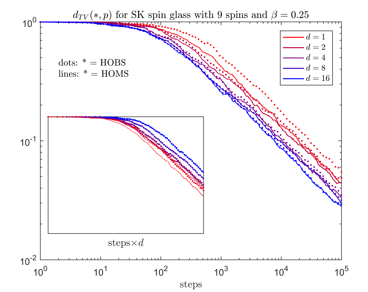
Figure 1: Total variation distance between the HOBS/HOMS with proposal sets $\mathcal{J}$ (elements distributed uniformly without replacement) of varying sizes $d$ and (24) with 9 spins and $\beta=1/4$. Inset: the same data and window, with horizontal axis normalized by $d$.

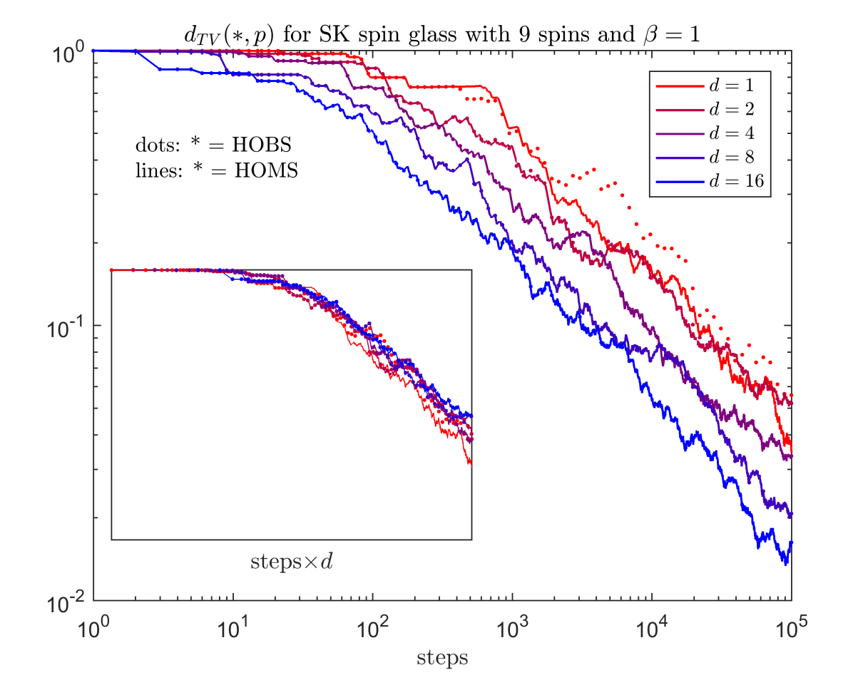
Figure 2: As in Figure 1 with $\beta=1$.

The SK model is well-suited for a straightforward evaluation of higher-order samplers because of its disordered energy landscape. More detailed models or benchmarks seem to require specific assumptions (e.g., the particular form of a spin Hamiltonian for Swendsen-Wang updates) and/or parameters (e.g., additional temperatures for parallel tempering, or of a vorticity matrix for non-reversible Metropolis-Hastings). In keeping with a straightforward evaluation, we do not consider sophisticated or diverse ways to generate elements of proposal sets $\mathcal{J}$. Instead, we simply select elements of $\mathcal{J}$ uniformly at random without replacement. We use the same pseudorandom number generator initial state for all simulations in order to highlight relative behavior. Finally, we choose $\beta$ low enough ($1/4$ and $1$) so that the behavior of a single run is sufficiently representative to make simple qualitative judgments.

The figure insets show that although higher-order samplers indeed converge more quickly, this comes at the cost of more overall evaluations of probability ratios. Parallelism is therefore necessary for higher-order samplers to be a wise algorithmic choice.

We reiterate in closing this section that the HOMS gives results very close to the HOBS, except for small values of $d$ or a more uniform target distribution $p$. Increasing the number of spins in the SK model and/or considering an Edwards-Anderson spin glass also yields qualitatively similar results (not shown here).

2.8 Linear objectives for transition matrices

We can push the preceding ideas further by using an optimization scheme to construct transition matrices with the desired invariant measures and that saturate a suitable objective function.

For example, the linear objective $-1_{\mathcal{J}}^{T}\tau_{(\mathcal{J})}^{(p)}r_{\mathcal{J}}^{T}$ considered immediately after (29) yields an optimal sparse approximation of the “ultimate” transition matrix $1p$. (To the best of our knowledge, this construction has not been considered elsewhere.) However, bringing an optimization scheme to bear narrows the regime of applicability to cases where computing likelihoods is hard enough and sufficient parallel resources are available to justify the added computational costs.

To make this concrete, first define $1_{\mathcal{J}}\in\mathbb{R}^{n}$ by

$$(1_{\mathcal{J}})_{j}:=\begin{cases}1&\text{if }j\in\mathcal{J}\cup\{n\}\\ 0&\text{otherwise},\end{cases}$$

$1_{\mathcal{J}}^{-}:=((1_{\mathcal{J}})_{1},\dots,(1_{\mathcal{J}})_{n-1})^{T}$, $r_{\mathcal{J}}:=r\odot 1_{\mathcal{J}}^{T}$, and $r_{\mathcal{J}}^{-}:=r^{-}\odot(1_{\mathcal{J}}^{-})^{T}$, where $\odot$ is the entrywise or Hadamard product (note that $r_{\mathcal{J}}\in\mathbb{R}^{n}$, while $r_{(\mathcal{J})}\in\mathbb{R}^{|\mathcal{J}|}$ has been defined previously).

Write $\Delta$ for the matrix diagonal map and recall the notation of Lemma 3: since

$$\tau_{(\mathcal{J})}^{(p)}=\begin{pmatrix}I_{n-1}\\ -r_{\mathcal{J}}^{-}\end{pmatrix}\tau\begin{pmatrix}I_{n-1}&-1_{\mathcal{J}}^{-}\end{pmatrix},$$ (25)

we have that $I-\tau_{(\mathcal{J})}^{(p)}\in\langle p\rangle^{+}$ iff

$$0 \leq I_{n-1}-\Delta(1_{\mathcal{J}}^{-})\tau\Delta(1_{\mathcal{J}}^{-})\leq 1;$$ (26a)

$$0 \leq\tau 1_{\mathcal{J}}^{-}\leq 1;$$ (26b)

$$0 \leq r_{\mathcal{J}}^{-}\tau\leq 1;$$ (26c)

$$0 \leq r_{\mathcal{J}}^{-}\tau 1_{\mathcal{J}}^{-}\leq 1.$$ (26d)

The constraints (26b)-(26d) respectively force the first $n-1$ entries of the last column, the first $n-1$ entries of the last row, and the bottom right matrix entry of $\tau_{(\mathcal{J})}^{(p)}$ to be in the unit interval. (26a) forces the relevant entries of the “coefficient matrix” $\tau$ (as an upper left submatrix of $\tau_{(\mathcal{J})}^{(p)}$) to be in the unit interval.

We can conveniently set to zero the irrelevant/unspecified rows and columns of $\tau$ that do not contribute to $\tau_{(\mathcal{J})}^{(p)}$ via the constraints

$$\Delta(1-1_{\mathcal{J}}^{-})\tau=\tau\Delta(1-1_{\mathcal{J}}^{-})=0.$$ (27)

Provided that we impose (27), (26a) can be replaced with

$$0\leq I_{n-1}-\tau\leq 1.$$ (28)

The “diagonal” case corresponding to Lemma 2 shows that (26) and (27) jointly have nontrivial solutions. This suggests that we consider suitable objectives and corresponding linear programs for optimizing the MCMC transition matrix $I-\tau_{(\mathcal{J})}^{(p)}$. We therefore introduce the vectorization map vec that sends a matrix to a vector by stacking matrix columns in order. This map obeys the useful identity $\text{vec}(XYZ^{T})=(Z\otimes X)\text{vec}(Y)$, where $\otimes$ denotes the Kronecker product.

Now a reasonably generic linear objective function is

$$x^{T}\tau_{(\mathcal{J})}^{(p)}y=(y^{T}\otimes x^{T})\text{vec}\left(\tau_{(\mathcal{J})}^{(p)}\right)$$ (29)

for suitable fixed $x$ and $y$. In practice, we consider $x=1_{\mathcal{J}}$ and $y=-r_{\mathcal{J}}^{T}$. This maximizes the Frobenius inner product of $I-\tau_{(\mathcal{J})}^{(p)}$ and $1_{\mathcal{J}}r_{\mathcal{J}}$ because

$$\text{Tr}\left(\left(I-\tau_{(\mathcal{J})}^{(p)}\right)^{T}1_{\mathcal{J}}r_{\mathcal{J}}\right)=r_{\mathcal{J}}1_{\mathcal{J}}-1_{\mathcal{J}}^{T}\tau_{(\mathcal{J})}^{(p)}r_{\mathcal{J}}^{T}.$$

Alternatives like $x=e_{n},y=e_{n}$ (to discourage self-transitions) can lead to convergence that slows catastrophically as $d=|\mathcal{J}|$ increases, because high-probability states are less likely to remain occupied. More surprisingly, the same sort of slowing down happens for $x=e_{n},y=-r_{\mathcal{J}}^{T}$, as well as for variations involving the $n$th component of $y$. We suspect that the cause is the same, albeit mediated indirectly through an objective that “overfits” the proposed transition probabilities to the detriment of remaining in place (or in some cases “underfits” by producing the identity matrix). Overall, it appears nontrivial to select better choices for $x$ and $y$ than our defaults above.

By (25) we get

$$\text{vec}\left(\tau_{(\mathcal{J})}^{(p)}\right)=\left[\begin{pmatrix}I_{n-1}\\ -(1_{\mathcal{J}}^{-})^{T}\end{pmatrix}\otimes\begin{pmatrix}I_{n-1}\\ -r_{\mathcal{J}}^{-}\end{pmatrix}\right]\text{vec}(\tau),$$ (30)

and in turn $(y^{T}\otimes x^{T})\text{vec}\left(\tau_{(\mathcal{J})}^{(p)}\right)$ equals

$$\left[y^{T}\begin{pmatrix}I_{n-1}\\ -(1_{\mathcal{J}}^{-})^{T}\end{pmatrix}\otimes x^{T}\begin{pmatrix}I_{n-1}\\ -r_{\mathcal{J}}^{-}\end{pmatrix}\right]\text{vec}(\tau).$$ (31)

Now the constraints and the objective of the linear program are both explicitly specified in terms of the “coefficient” matrix $\tau$, so in principle we have a working algorithm already. However, it is convenient to respectively rephrase the constraints (26b)-(26d), (27), and (28) into different forms as

$$0\leq\begin{pmatrix}\left(1_{\mathcal{J}}^{-}\right)^{T}\otimes I_{n-1}\\ I_{n-1}\otimes r_{\mathcal{J}}^{-}\\ \left(1_{\mathcal{J}}^{-}\right)^{T}\otimes r_{\mathcal{J}}^{-}\end{pmatrix}\text{vec}(\tau)\leq 1,$$ (32)

$$\begin{pmatrix}I_{n-1}\otimes\Delta(1-1_{\mathcal{J}}^{-})\\ \Delta(1-1_{\mathcal{J}}^{-})\otimes I_{n-1}\end{pmatrix}\text{vec}(\tau)=0,$$ (33)

$$\text{vec}(I_{n-1})-1\leq\text{vec}(\tau)\leq\text{vec}(I_{n-1}).$$ (34)

Therefore, writing

$$U_{(\mathcal{J})}^{(p)}:= \ \begin{pmatrix}I_{2n-1}\\ -I_{2n-1}\end{pmatrix}\begin{pmatrix}\left(1_{\mathcal{J}}^{-}\right)^{T}\otimes I_{n-1}\\ I_{n-1}\otimes r_{\mathcal{J}}^{-}\\ \left(1_{\mathcal{J}}^{-}\right)^{T}\otimes r_{\mathcal{J}}^{-}\end{pmatrix};$$

$$v:= \ \begin{pmatrix}1_{2n-1}\\ 0_{2n-1}\end{pmatrix};$$

$$w_{(\mathcal{J})}^{(p)}:= \ -y^{T}\begin{pmatrix}I_{n-1}\\ -(1_{\mathcal{J}}^{-})^{T}\end{pmatrix}\otimes x^{T}\begin{pmatrix}I_{n-1}\\ -r_{\mathcal{J}}^{-}\end{pmatrix},$$

and

$$U_{(\mathcal{J})}^{(0)}:=\begin{pmatrix}I_{n-1}\otimes\Delta(1-1_{\mathcal{J}}^{-})\\ \Delta(1-1_{\mathcal{J}}^{-})\otimes I_{n-1}\end{pmatrix},$$ (35)

we can at last write the sought-after linear program (noting a minus sign included in $w_{(\mathcal{J})}^{(p)}$) in a form suitable for (e.g.) MATLAB’s linprog solver:

$$\min_{\tau}w_{(\mathcal{J})}^{(p)}\text{vec}(\tau)\quad\text{s.t.}$$

$$U_{(\mathcal{J})}^{(p)}\text{vec}(\tau)\quad\leq \quad v;$$ (36a)

$$U_{(\mathcal{J})}^{(0)}\text{vec}(\tau)\quad= \quad 0;$$ (36b)

$$\text{vec}(\tau)\quad\geq \quad\text{vec}(I_{n-1})-1;$$ (36c)

$$\text{vec}(\tau)\quad\leq \quad\text{vec}(I_{n-1}).$$ (36d)

The preceding discussion therefore culminates in the following

Theorem 2.3

The linear program (36) has a solution in $\langle p\rangle^{+}$. ∎

Example

As in §2.5, consider $p=(1,2,3,4,10)/20$ and $\mathcal{J}=\{1,2,3\}$. Solving the linear program with $x=1_{\mathcal{J}}$ and $y=-r_{\mathcal{J}}^{T}$ produces the following element of $\langle p\rangle^{+}$:

$$\begin{pmatrix}0&0&0&0&1\\ 0&0&0&0&1\\ 0&0&0&0&1\\ 0&0&0&1&0\\ 0.1&0.2&0.3&0&0.4\end{pmatrix}.$$

For comparison, recall that the last row of $\mathcal{M}_{(\mathcal{J})}^{(p)}$ equals $(0.0\bar{6},0.1\bar{3},0.2,0,0.6)$.

The higher-order programming sampler

We call the sampler obtained from (29) and (36) with $x=-1_{\mathcal{J}}$ and $y=r_{\mathcal{J}}^{T}$ the higher-order programming sampler (HOPS). We compare the HOMS and HOPS in Figures 3 and 4 (cf. Figures 1 and 2). The figures show that the HOPS improves upon the HOMS, which in turn improves upon the HOBS.

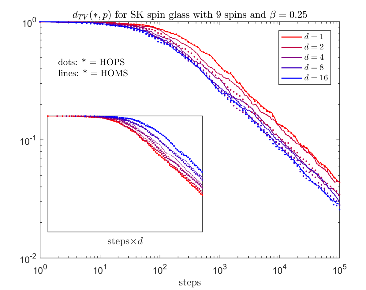
Figure 3: Total variation distance between the HOPS/HOMS with proposal sets $\mathcal{J}$ (elements sampled uniformly without replacement) of varying sizes $d$ and (24) with 9 spins and $\beta=1/4$. Inset: same data and window, with horizontal axis normalized by $d$.

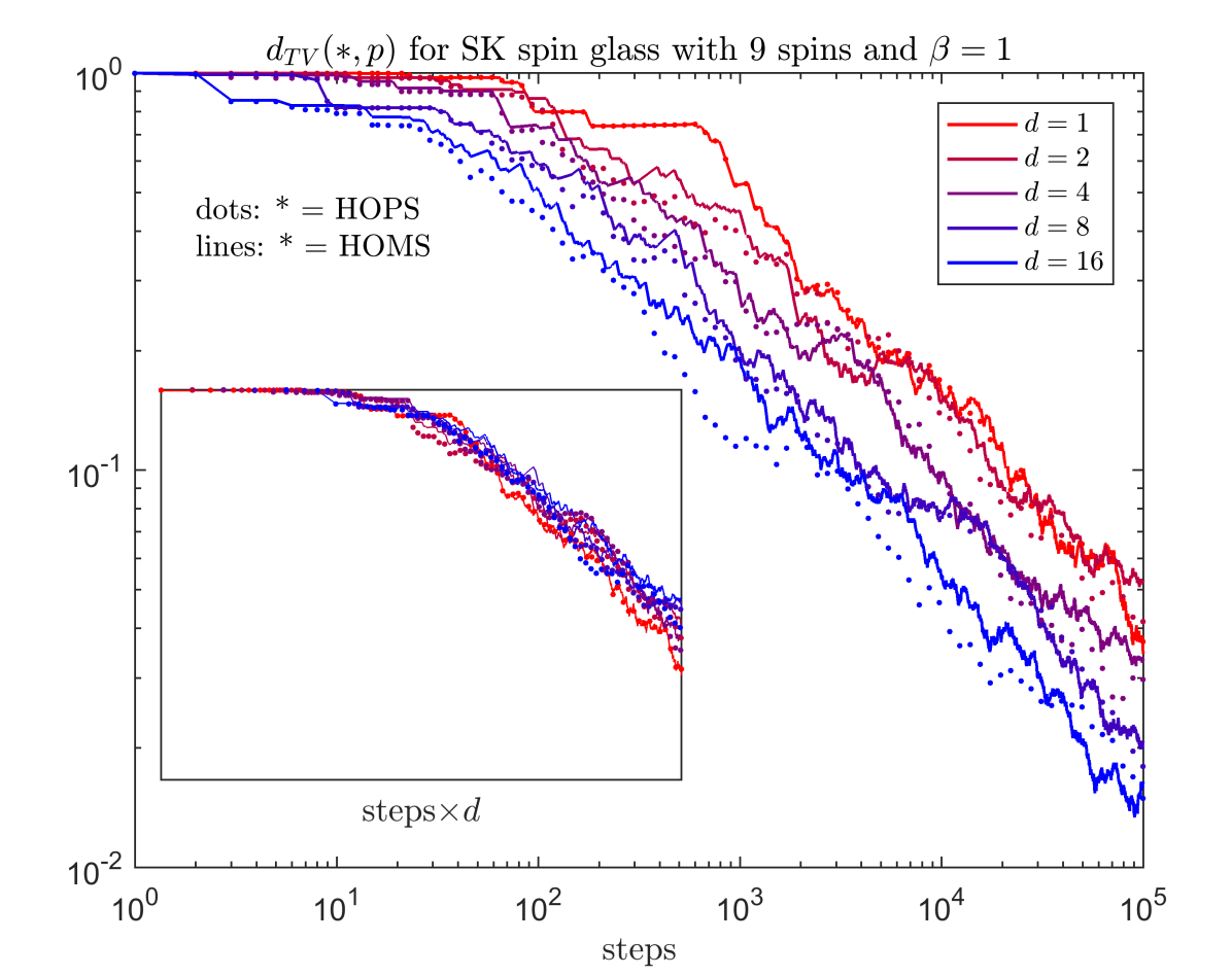
Figure 4: As in Figure 3 with $\beta=1$.

Algorithm 4 HOPS

  Input: Runtime $T$ and oracle for $r$

  Initialize $t=0$ and $X_{0}$

  repeat

     Relabel states so that $X_{t}=n$

     Propose $\mathcal{J}=\{j_{1},\dots,j_{d}\}\subseteq[n-1]$

     Compute $\tau$ solving (36) with $x=1_{\mathcal{J}}$ and $y=-r_{\mathcal{J}}^{T}$

     Set $P=I-\tau_{(\mathcal{J})}^{(p)}$ using (25)

     Accept $X_{t+1}=j_{u}$ with probability $P_{nj_{u}}$

     Undo relabeling; set $t=t+1$

  until $t=T$

  Output: $\{X_{t}\}_{t=0}^{T}\sim p^{\times(T+1)}$ (approximately)

2.9 Remarks on sampling

Besides providing a framework that conceptually unifies various MCMC algorithms, symmetry principles lead to the apparently new HOPS algorithm of §2.8. It is possible that the HOPS itself might be further improved upon by developing an objective function suited for, e.g. convex optimization versus a mere linear program. These ideas might also enhance existing MCMC techniques specifically tailored for parallel computation, as in conrad2018expensive . In particular, the Bayesian approach to inverse problems dashti2016inverse may be fertile ground for applications.

As we have already mentioned, our approach is agnostic with respect to proposals, focusing purely on acceptance mechanisms. However, the proposal mechanism has less impact than the acceptance mechanism in practice, especially for differentiable distributions. In practice, a stateful and/or problem-specific proposal exploiting joint structure is highly desirable and even necessary for any real utility, but we these avenues unexplored for now (one possibility is suggested by particle MTMS algorithms as in martino2014 and exploiting tensor product structure in transition matrices and $\langle p\rangle$). It would be of interest to incorporate some aspect of a proposal mechanism into the objective of (36), but it is not clear how to actually do this. In fact, our numerical example featured a SK spin glass to illustrate our ideas precisely because its highly disordered structure (and discrete state space) are suited for separating concerns about proposal and acceptance mechanisms.

It would certainly be interesting to extend the present considerations to continuous variables. However, this would seem to require a more technical treatment, since infinite-dimensional Lie theory, distributions à la Schwartz, etc. would play a role at least in principle. In a complementary vein, it would be interesting to see if the full construction of delmas2009does could be recovered from symmetry arguments alone.

While the Barker and Metropolis samplers are reversible, it is not clear if the HOPS is, though bierkens2016nonreversible points out ways to transform reversible kernels into irreversible ones and vice versa.

It is possible to produce transition matrices (even in closed form) in which the $n$th row is nonnegative but other rows have negative entries. It is not immediately clear if using such a matrix actually poisons a MCMC algorithm. Though preliminary experiments in this direction were discouraging, we have not found a compelling argument that rules out the use of such matrices.

Finally, it would be of interest to sample from the vertices of the polytope $\langle p\rangle^{+}$. However, (even approximately) uniformly sampling vertices of a polytope is $\mathbf{NP}$-hard (and thus presumably intractable) by Theorem 1 of khachiyan2001transversal : see also khachiyan2008vertices .

3 Statistical physics via symmetry

We have seen in §2 that sampling algorithms can be better understood in principle and also accelerated in practice through elementary considerations of symmetry. In the present section, we show how similarly basic considerations of symmetry can derive the basic structure of statistical physics. While we do not address entropy per se, that ground is well-traveled, with the well-known characterization of Faddeev faddeev1956concept ; baez2011characterization playing an exemplary role.

We focus instead on the role of temperature (and via closure of the Gibbs relation, energy), which classical information-theoretical considerations have not substantially accounted for. In particular, we sketch how an effective temperature can reproduce the physical temperature for conjecturally generic model systems (see also §4), while also enabling applications to data analytics, characterization of time-inhomogeneous Markov processes, nonequilibrium thermodynamics, etc.

The goal of providing a self-consistent description of stationary systems with finitely many states using the language of equilibrium statistical physics in the canonical ensemble naturally flows from the idea expressed in gallavotti2008heat that “there is no conceptual difference between stationary states in equilibrium and out of equilibrium.” While the traditional aim of statistical physics is predicting statistical behavior in terms of measured physical properties, the aim here is to go in the other direction: that is, to determine effective physical properties–in and out of equilibrium–in terms of observable statistical behavior. In other words, the goal is to take one step farther the now-classical maximum entropy point of view in which statistical physics is a framework for reasoning about data.

We realize this goal by demonstrating the existence, uniqueness (up to a choice of scale), and relevance of a physically reasonable and invertible transformation between simple effective statistical and physical descriptions of a system (see figure 5). The effective statistical description is furnished by a probability distribution along with a characteristic timescale. The effective physical description consists of an effective energy function and an effective temperature. The transformation between these descriptions will be derived from the elementary Gibbs relation and basic symmetry considerations along lines first explored in ford2005surfaces ; ford2006descriptive .

The utility and naturalness of the effective physical description that results from performing this transformation on an effective statistical description will depend entirely on the utility and naturalness of the underlying state space and of the characteristic timescale. In the event that the actual state space of a real physical system in thermal equilibrium is finite and an appropriate characteristic timescale can be determined, the corresponding effective physical description will manifestly reproduce the actual physics. Moreover, in near-equilibrium, the effective temperature and energies will remain near the actual values of their equilibrium analogues by a continuity argument. Consequently, the framework discussed here may inform principled characterizations of quasi-equilibria.

However, as the system is driven away from equilibrium, its effective energy levels will shift, while the actual energy levels of a real physical system may be fixed and intrinsic. Nevertheless, such shifts are still of interest for characterizing nonequilibrium situations, even for real physical systems. For example, a system such as a laser undergoing population inversion will exhibit an effective level crossing as the driving parameter varies. In a related vein, a negative absolute temperature braun2013negative ; dunkel2014consistent ; frenkel2015gibbs would correspond in our framework to a negative characteristic timescale, indicating antithermodynamic behavior such as “antimixing” or “antirelaxation.”

Even very limited knowledge about the energy levels and temperature of a system is sufficient to determine the remainder of that information as a trivial exercise in algebra using the Gibbs relation. Nevertheless, the preceding discussion should not distract from the observation that the framework discussed here provides its most substantial advantage in the situation where inverting the Gibbs relation might initially seem like an ill-posed problem. Therefore, the primary goal of the framework discussed below is to give effective physical descriptions of systems that have no a priori physical characterization, while maintaining total consistency with equilibrium statistical physics in situations where an a priori physical characterization is available.

Highlighting this consistency is the example of Anosov systems (see §4), and specifically paradigmatic chaotic model systems such as the cat map and the free particle or ideal gas on a surface of constant negative curvature, where using a careful iterative discretization scheme indicates how the actual energy and temperature may be reproduced by suitable effective analogues, despite the fact that the underlying state spaces are continuous. Thermostatting subsequently indicates how the transformation at the heart of our discussion could be applied in principle to essentially arbitrary physical systems huntsman2010anosov .

While the perspective we shall take below does not confer extensive predictive power in the realm of physics, it does have some (see, e.g. §3.8) and its descriptive and explanatory power nevertheless suggests a wide and significant scope for applications, including to nonequilibrium statistical physics, the renormalization group, information theory, and the characterization of both stochastic processes and experimental data. More provocatively, it can be regarded as illuminating the fundamental meaning of both energy and temperature independently of references to work, force, mass, or the underlying spatial context upon which the latter concepts ultimately depend for their definition.

In this section, we derive the Gibbs relation from symmetry considerations in §3.1 before introducing the coordinate systems that respectively underlie experimental/probabilistic and theoretical/physical descriptions of systems in §3.2. With the stage set, we perform some preliminary algebra in §3.3. After obtaining intermediate results on the scaling behavior of inverse temperature as a function of time in §3.4 and on the geometry of any reasonable transformation between the two descriptions above in §3.5, we complete the derivation of the effective temperature in §3.6. We then outline constraints on the form of a characteristic timescale imposed by considering product systems in §3.7. Finally, we outline a number of examples and applications in §3.8 before remarks in §3.9.

Later, §4 considers the effective temperature for Anosov systems.

At times, we may write $\beta$ to denote the physical or actual inverse temperature as well as an effective analogue. Context should serve to eliminate any ambiguity, especially as we make an effort to separate discussion of these two quantities impinging on equations.

3.1 The Gibbs distribution

The first step in deriving the basic structure of statistical physics from symmetry is to derive the Gibbs relation between state probabilities and energies. We do this for a finite system from the basic postulate that the probability of a state depends only on its energy. This derivation will implicitly motivate the construction of the effective temperature that culminates in §3.6. While unlike more classical derivations ours does not motivate the introduction of entropy, the standard information-theoretic motivation provides a more than adequate remedy, and the Faddeev characterization of entropy is also a symmetry argument faddeev1956concept ; baez2011characterization .

The key observation is that energy is only defined up to an additive constant, i.e., only energy differences are physically meaningful. This and the basic postulate that state probabilities are functions of state energies together imply that

$$\mathbb{P}(E_{k})=\frac{f(E_{k})}{\sum_{j}f(E_{j})}=\frac{f(E_{k}+\varepsilon)}{\sum_{j}f(E_{j}+\varepsilon)}$$ (37)

for some function $f$ and $\varepsilon$ arbitrary. Define

$$g_{E}(\varepsilon):=\frac{\sum_{j}f(E_{j}+\varepsilon)}{\sum_{j}f(E_{j})}$$ (38)

and note that $g_{E}(0)=1$ by definition. It follows that

$$\mathbb{P}(E_{k})=\frac{f(E_{k})}{\sum_{j}f(E_{j}+\varepsilon)}g_{E}(\varepsilon)=\frac{f(E_{k}+\varepsilon)}{\sum_{j}f(E_{j}+\varepsilon)}.$$ (39)

Therefore $g_{E}(\varepsilon)f(E_{k})=f(E_{k}+\varepsilon)$, implying that

$$f(E_{k}+\varepsilon)-f(E_{k})=(g_{E}(\varepsilon)-1)\cdot f(E_{k}).$$ (40)

Since $g_{E}(0)=1$, we obtain $f^{\prime}(E_{k})=g^{\prime}_{E}(0)f(E_{k})$, and in turn

$$f(E_{k})=C\exp(g^{\prime}_{E}(0)E_{k}).$$ (41)

Without loss of generality, we can set $\beta:=-g^{\prime}_{E}(0)$ and $C\equiv 1$, which produces the Gibbs distribution so long as the temperature is defined as $\beta^{-1}$.

We note that the present derivation can be made rigorous (e.g., details involving continuity and the Cauchy functional equation) without substantial difficulty, but also without substantive additional insight. Also, $g_{E}(\varepsilon)=\exp(-\beta\varepsilon)$ so that $g_{E}\equiv g$, as required for the self-consistency of the argument. Although the present derivation is only appropriate for $\beta$ fixed, this just amounts to considering the canonical ensemble in the first place.

Finally, we reiterate that there are just a handful of symmetry and scaling principles collectively underlying the present derivation and that of the effective temperature below. In concert with the standard information-theoretical infrastructure for entropy, these principles provide an exceptionally parsimonious framework for the equilibrium statistical physics of finite systems.

3.2 Statistical and physical system descriptions

Consider now a stationary system with state space $[n]$. For our purposes, a sufficient statistical description of such a system is provided by the $(n+1)$-tuple $(p_{1},\dots,p_{n},t_{\infty})=(p,t_{\infty})$, where $p_{j}:=\mathbb{P}(s(t)=j)$ is the probability for the system to be in state $j\in[n]$, and where $t_{\infty}$ is a suitable characteristic or “effective” timescale. Defining $t_{j}:=t_{\infty}p_{j}$, the $n$-tuple $t:=t_{\infty}p=(t_{1},\dots,t_{n})$ provides an alternative but completely equivalent description of the system, since the probability constraint $\sum_{j}p_{j}=1$ implies that $t_{\infty}=\sum_{j}t_{j}$. We will use both of these descriptions interchangeably below without further comment.

Meanwhile, a sufficient physical description of the system is provided by the $(n+1)$-tuple $H:=(E_{1},\dots,E_{n},\beta^{-1})=(E,\beta^{-1})$, where $E_{j}$ is an effective energy for state $j$, and where $\beta$ is an effective inverse temperature. It will also be convenient to introduce $\gamma:=\beta E$, noting that $\beta H=(\gamma,1)$.

Below, we will construct well-defined and essentially unique physically reasonable and mutually inverse maps (see Figure 5)

$$F_{H}(t)=H,\quad F_{t}(H)=t.$$ (42)

The map $F_{t}$ extends the familiar Gibbs relation (44), and the relationship between $t_{\infty}$ and $\beta$ plays a pivotal role in the construction of both $F_{H}$ and $F_{t}$. In particular, we will determine $\beta$ as a function of $t$ in (66), whereupon the Gibbs relation and equation (43) for the reference energy will complete the detailed specification of $F_{H}$.

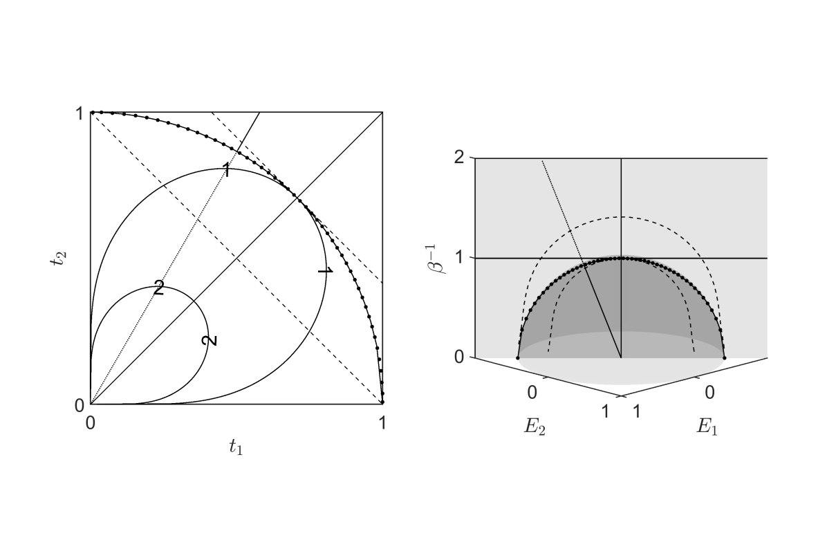
Figure 5: Geometry of the maps (42) for $n=2$ states. Level curves of $\beta^{-1}=1,2$ (solid contours) and of $t_{\infty}=1,\sqrt{2}$ (dashed contours) are shown in both coordinate systems. The actions of the maps are also shown explicitly for circular arcs and rays.

Because adding an arbitrary constant to the effective state energies merely amounts to a shift of a potential with no physical relevance, it is convenient to specify a reference energy, at least temporarily. With the preceding considerations in mind, and without any loss of generality, we impose the constraint

$$\frac{1}{n}\sum_{j}E_{j}=0.$$ (43)

Note that we may later enforce any other convenient reference energy, e.g., $\min_{j}E_{j}\equiv 0$, $n^{-1}\sum_{j}E_{j}=\beta^{-1}$, etc.

3.3 Preliminary algebra

For systems in thermal equilibrium, it is natural to require that $\beta$ is the inverse of the physical temperature, i.e., that the effective and physical temperatures coincide. In this case the fundamental principle of equilibrium statistical physics embodied by the Gibbs relation may be expressed as

$$p_{k}=Z^{-1}e^{-\gamma_{k}}$$ (44)

and regarded as a map $p=F_{p}(H)$. Here as usual $Z:=\sum_{j}e^{-\gamma_{j}}$ is the partition function.

By provisionally ignoring whether or not a generic stationary system is actually in thermal equilibrium, (44) can be viewed as a constraint linking its physical and statistical descriptions. We will justify this interpretation below by using elementary symmetries and scaling relationships to specify (up to an overall constant) the inverse $F_{H}$ of an augmentation $F_{t}$ of the Gibbs map $F_{p}$.

Taking logarithms on both sides of (44) yields

$$-\log Z-\gamma_{k}=\log p_{k}.$$ (45)

Meanwhile, the constraint (43) implies that $n^{-1}\sum_{j}\gamma_{j}=0$. Combining this observation with arithmetic averaging of both sides of (45) leads to the result

$$-\log Z=\frac{1}{n}\sum_{j}\log p_{j}.$$ (46)

Substituting (46) into (45) and solving for $\gamma_{k}$ shows that

$$\gamma_{k}=\frac{1}{n}\sum_{j}\log p_{j}-\log p_{k}.$$ (47)

Since $\beta F_{H}(t)=(\gamma,1)$,

$$\lVert\beta F_{H}(t)\rVert^{2}=\lVert\gamma\rVert^{2}+1,$$ (48)

where $\lVert\cdot\rVert$ denotes the usual Euclidean norm. That is, $\lVert\beta F_{H}(t)\rVert=\sqrt{\lVert\gamma\rVert^{2}+1}$ can be explicitly computed in terms of $\gamma$ (and by (47) also in terms of $p$) alone.

Therefore, in order to determine $\beta$, it remains chiefly to determine $\lVert F_{H}(t)\rVert$, since $\lVert\beta F_{H}(t)\rVert$ is known from (48) and we tautologically have that

$$\beta=\lVert\beta F_{H}(t)\rVert/\lVert F_{H}(t)\rVert.$$ (49)

To determine $\lVert F_{H}(t)\rVert$, we will establish two results on scaling and geometry next.

3.4 A scaling result

Dimensional considerations imply that if $\beta$ is determined by any well-behaved map $F_{H}$, then it must depend on some constant governing parameter $S$ in addition to $t$. That is, $\beta=f(t;S)$. By the Buckingham $\Pi$-theorem buckingham1914physically ; barenblatt2003scaling , $\beta=S^{\xi}t_{\infty}^{\omega}\Psi(p)$ for some $\xi$ and $\omega$, where $\Psi$ is dimensionless.

Consider for the moment a system governed by a Hamiltonian $\mathcal{H}(X,P)$. If $C$ is a constant, the transformation $t\mapsto t^{\prime}:=t/C$ induces the transformation $t_{\infty}\mapsto t^{\prime}_{\infty}:=t_{\infty}/C$ as well as the extended canonical (pure scale) transformation goldstein2001classical

$$X\mapsto X^{\prime}=X,\quad P\mapsto P^{\prime}=CP,\quad\mathcal{H}\mapsto\mathcal{H}^{\prime}=C\mathcal{H}.$$ (50)

Since the transformation (50) can be considered as a change of units, it necessarily leaves the actual (vs. effective) Gibbs factor $e^{-\beta\mathcal{H}}$ invariant. That is, $\beta\mathcal{H}=\beta^{\prime}\mathcal{H}^{\prime}=\beta^{\prime}C\mathcal{H}$. This observation immediately yields that $\beta\mapsto\beta^{\prime}=\beta/C$. Physical consistency therefore demands that

$$F_{H}(t/C)=C\cdot F_{H}(t).$$ (51)

From this, it follows that $\omega=1$, so without loss of generality

$$\beta=S^{-1}t_{\infty}\Psi(p),$$ (52)

where the constant $S$ carries units of action (say, $S=\hbar$).

Additional arguments in support of (51) and (52)

A reader fully convinced by the argument just above can safely skip this section.

Ideal gas systems

Consider a Gedankenexperiment with two systems, comprised respectively of finite ideal gas samples with particle masses $m$ and $m^{\prime}=m/C$, each in identical freefalling containers in contact with isotropic thermal baths, and with the same initial conditions in phase space. Let $P=P^{\prime}$ denote the common rms momentum of particles in both systems: the respective inverse temperatures of the two systems are then in common proportion to $m/P^{2}$ and $m^{\prime}/P^{\prime 2}=(m/C)/P^{2}$.

Insofar as the system microstates are not of interest in equilibrium, the systems may be respectively described by, e.g. the quintuples $(m,v,P,t_{\infty},\beta)$ and $(m^{\prime},v^{\prime},P^{\prime},t_{\infty}^{\prime},\beta^{\prime})=(m/C,Cv,P,t_{\infty}/C,\beta/C)$, where $v^{(\cdot)}$ denotes a rms velocity and here $t_{\infty}^{(\cdot)}$ denotes any characteristic timescale of the same nature in both systems.

Both systems follow the same trajectory through phase space, albeit at rates that differ by constant factors, and we see that $\beta$ scales as $t_{\infty}$ for ideal gases, and hence (by coupling with an ideal gas bath) for general systems also. Therefore, consistency with elementary equilibrium statistical physics requires that $\beta$ also scales as $t_{\infty}$.

The classical KMS condition

Another argument along similar lines to that in §3.4 for the scaling behavior of $\beta$ w/r/t $t_{\infty}$ directly invokes the classical Kubo-Martin-Schwinger (KMS) condition. To begin, we recall the usual (quantum) KMS condition before formally deriving its classical analogue in the limit $\hbar\rightarrow 0$ by way of background.

A quantum Hamiltonian $\mathcal{\hat{H}}$ has thermal density matrix

$$\hat{\rho}:=Z^{-1}e^{-\beta\mathcal{\hat{H}}},$$ (53)

where $Z:=\mbox{Tr}(e^{-\beta\mathcal{\hat{H}}})$, and the time evolution of an observable $\hat{A}$ in the Heisenberg picture is given as usual by $\tau_{t}(\hat{A}):=e^{i\mathcal{\hat{H}}t/\hbar}\hat{A}e^{-i\mathcal{\hat{H}}t/\hbar}$.

The quantum Gibbs rule $\langle\hat{A}\rangle=\mbox{Tr}(\hat{\rho}\hat{A})$, with $\hat{\rho}$ given by (53), is generalized by the KMS condition gallavotti1975classical ; parisi1998statistical

$$\left\langle\tau_{t}(\hat{A})\hat{B}\right\rangle=\left\langle\hat{B}\tau_{t+i\hbar\beta}(\hat{A})\right\rangle.$$ (54)

For convenience, we recall a formal derivation of (54) from the Gibbs rule and the cyclic property of the trace:

$$\left\langle\tau_{t}(\hat{A})\hat{B}\right\rangle = Z^{-1}\mbox{Tr}(e^{-\beta\mathcal{\hat{H}}}e^{i\mathcal{\hat{H}}t/\hbar}\hat{A}e^{-i\mathcal{\hat{H}}t/\hbar}\hat{B})$$

$$= Z^{-1}\mbox{Tr}(\hat{B}e^{i\mathcal{\hat{H}}z/\hbar}\hat{A}e^{-i\mathcal{\hat{H}}t/\hbar})$$

$$= Z^{-1}\mbox{Tr}(\hat{B}e^{i\mathcal{\hat{H}}z/\hbar}\hat{A}e^{-i\mathcal{\hat{H}}z/\hbar}e^{-\beta\mathcal{\hat{H}}})$$

$$= \left\langle\hat{B}\tau_{z}(\hat{A})\right\rangle$$

where here we have written $z:=t+i\hbar\beta$.

Following gallavotti1975classical , we have by (54) the following precursor to the classical KMS condition:

$$\left\langle\frac{[\tau_{t}(\hat{A}),\hat{B}]}{i\hbar}\right\rangle=\left\langle\hat{B}\left(\frac{\tau_{z}(\hat{A})-\tau_{t}(\hat{A})}{i\hbar}\right)\right\rangle.$$ (55)

Recall that as $\hbar\rightarrow 0$, $\tau_{t}(\hat{A})$, $\hat{B}$ and $[\tau_{t}(\hat{A}),\hat{B}]/i\hbar$ respectively correspond to or “undeform” into classical analogues $A$, $B$ and $\{A,B\}$, where $A$ has an implicit time dependence (i.e., $\partial_{t}A=0\not\equiv dA/dt$) and $B$ does not (i.e., $B$ is evaluated at $t=0$).

Now (via an implicit assumption about the analyticity of $\tau_{z}$ which forms the actual substance of the KMS condition) we have that

$$\lim_{\hbar\rightarrow 0}\frac{\tau_{z}(\hat{A})-\tau_{t}(\hat{A})}{i\hbar}=\beta\frac{dA}{dt}=\beta\{A,\mathcal{H}\}$$ (56)

where $\mathcal{H}(X,P)$ is the classical Hamiltonian. Therefore in the limit $\hbar\rightarrow 0$, (55) formally becomes the classical KMS condition (see also parisi1998statistical )

$$\left\langle\{A,B\}\right\rangle=\beta\left\langle B\{A,\mathcal{H}\}\right\rangle.$$ (57)

As in §3.4, here let $t_{\infty}^{(\cdot)}$ denote any characteristic timescale of the system. Dilating the dynamical rate by a constant factor $C$ has the effect that $t_{\infty}\mapsto t^{\prime}_{\infty}=t_{\infty}/C$ and also induces the extended canonical (pure scale) transformation (50). It follows that $\partial_{X}=\partial_{X^{\prime}}$ and $\partial_{P}=C\partial_{P^{\prime}}$, whence $\{A,B\}=C\{A,B\}^{\prime}$ and $\{A,\mathcal{H}\}=C\{A,C^{-1}\mathcal{H}\}^{\prime}=\{A,\mathcal{H}^{\prime}\}^{\prime}$ (here $\{\cdot,\cdot\}^{\prime}$ denotes the Poisson bracket w/r/t $(X^{\prime},P^{\prime})$). Along with (57), this in turn gives that

$$\beta=\frac{\left\langle\{A,B\}\right\rangle}{\left\langle B\{A,\mathcal{H}\}\right\rangle}=\frac{\left\langle C\{A,B\}^{\prime}\right\rangle}{\left\langle B\{A,\mathcal{H}^{\prime}\}^{\prime}\right\rangle}=C\beta^{\prime}.$$ (58)

Therefore $\beta^{\prime}=\beta/C$ and we see once more that $\beta$ scales as any characteristic time $t_{\infty}$. Again, consistency with traditional equilibrium statistical physics dictates that an effective inverse temperature should also scale as $t_{\infty}$.

Thermal time hypothesis

The one-parameter modular group of $\hat{\rho}$ (as defined in (53)) that appears in the Tomita-Takesaki theory of von Neumann algebras bratteli2012operator can be shown to coincide with the time evolution group connes1994neumann : if $s$ is the modular parameter and $t$ is the physical time, then

$$t=\hbar\beta s.$$ (59)

In particular, $s$ does not depend on $\beta$.

The thermal time hypothesis (TTH) articulated by Connes and Rovelli connes1994neumann (see also martinetti2003diamond ; rovelli1993statistical ; tian2005sitter ; rovelli2011thermal ) states that physical time is determined by the modular group, which is in turn determined by the state.

Besides implying Hamiltonian mechanics, the TTH simultaneously inverts and generalizes the KMS condition (see §3.4) and hence also the Gibbs relation (44), with temperature providing the physical link between time evolution and equilibria. But its key implication here is (59), by which $\beta$ scales as any characteristic time $t_{\infty}$; as before consistency demands the same scaling behavior for an effective inverse temperature.

Counterarguments for alternative scaling behavior

Despite the scaling arguments presented above, we might nevertheless feel compelled to consider alternative scaling behavior, with an effective inverse temperature of the form $\|t\|^{\omega}\sqrt{\|\gamma\|^{2}+1}$. However, for $\omega\neq 1$ this quantity does not converge in a natural way for archetypal Anosov systems (see §4), nor by extension does it appear to be relevant to the example of a two-dimensional ideal gas. Furthermore, its physical relevance for a single Glauber-Ising spin (see §3.8) is dubious for $\omega\neq 1$. Such behavior can be viewed as providing additional (albeit more circumstantial) evidence for an effective inverse temperature scaling as $t_{\infty}$, as can the validity of the Ansatz suggested by this scaling behavior for synchronization frequencies of Kuramoto oscillators (see 3.8).

3.5 A geometry result

The transformation $t\mapsto t^{\prime}:=t/C$ leaves $p$ invariant. Meanwhile, $\gamma_{k}$ depends only on $p$, so both $\gamma$ and $\beta H=(\gamma,1)$ are also invariant under this transformation, in accordance with (51). In other words, $p$ is positive homogeneous of degree zero in both $t$ and $H$, i.e., $F_{p}(Ct):=t/t_{\infty}=F_{p}(t)$ and $F_{p}(CH)=F_{p}(H)$.

Recall that Euler’s homogeneous function theorem states that if $f\in C^{1}(\mathbb{R}_{+}^{n})$ is positive homogeneous of degree $a$, then $\langle x,\nabla_{x}f(x)\rangle=a\cdot f(x)$ reiss1997methods . Since each component $p_{k}$ of $p$ is positive homogeneous of degree zero as a function of both $t$ and $H$, it follows that $\langle\nabla_{t}p_{k},t\rangle=0=\langle\nabla_{H}p_{k},H\rangle$. Therefore each of the gradients $\nabla_{t}p_{k}$ and $\nabla_{H}p_{k}$ are tangent to spheres centered at the origin of their respective coordinate systems.

Furthermore, the gradients $\nabla_{t}p_{k}$ and $\nabla_{H}p_{k}$ are nondegenerate: an explicit calculation shows that $\partial p_{k}/\partial E_{j}=\beta p_{k}(-\delta_{jk}+p_{j})\neq 0$, and $\partial p_{k}/\partial(\beta^{-1})=\beta^{2}p_{k}(E_{k}-U)$, where as usual $U:=\sum_{j}p_{j}E_{j}$. Meanwhile, $\partial p_{k}/\partial t_{j}=(\delta_{jk}t_{\infty}-t_{k})/t_{\infty}^{2}\neq 0$. Taking appropriate directional derivatives makes it easy to see that the constraint (43) does not affect the nondegeneracy of these gradients.

Consider now the unique decomposition of a vector differential as $dv=dv^{\parallel}+dv^{\perp}$, where the terms on the right hand side are respectively parallel and perpendicular to $v$. That is, $dv^{\parallel}:=(\langle dv,v\rangle/\langle v,v\rangle)v$, and $dv^{\perp}:=v-dv^{\parallel}$. It is easy to see that $dt^{\perp}=0\iff dp=0\iff dH^{\perp}=0$ from the preceding considerations. Moreover, $\langle\nabla_{t^{\perp}}p_{k},dt^{\perp}\rangle=\langle\nabla_{t}p_{k},dt\rangle=dp_{k}=\langle\nabla_{H}p_{k},dH\rangle=\langle\nabla_{H^{\perp}}p_{k},dH^{\perp}\rangle$. That is, the nondegenerate integral curves of both gradient flows are arcs on spheres centered at the origin. Since a smooth change of coordinates maps integral curves into integral curves choquet1977analysis , it follows that the respective spheres on which these arcs lie must also map to each other under any smooth maps $F_{H}$ and $F_{t}$ satisfying (43) and (44). We therefore have

Lemma 5

A well-behaved map $F_{H}$ that respects (43) and (44) sends rays and sphere orthants centered at the origin to rays and hemispheres centered at the origin, respectively. In particular, a well-behaved map $F_{H}$ that respects (43) and (44) must satisfy

$$\lVert{\bm{s}}\rVert=\lVert t\rVert\Rightarrow\lVert F_{H}({\bm{s}})\rVert=\lVert F_{H}(t)\rVert.$$ (60)

3.6 The effective temperature

Let $u_{j}:=\lVert t\rVert/\sqrt{n}$, so that $\lVert u\rVert\equiv\lVert t\rVert$ and $F_{H}(u)\equiv(0,\dots,0,\beta_{u}^{-1})$. Now $\lVert F_{H}(u)\rVert^{2}=\beta_{u}^{-2}$, and by (60)

$$\lVert F_{H}(t)\rVert^{2}=\lVert F_{H}(u)\rVert^{2}=\beta_{u}^{-2}.$$ (61)

Therefore, by (48) and (49),

$$\beta^{2}=\frac{\lVert\beta F_{H}(t)\rVert^{2}}{\lVert F_{H}(t)\rVert^{2}}=\frac{\lVert\gamma\rVert^{2}+1}{\beta_{u}^{-2}}.$$ (62)

Taking square roots of the far left- and right-hand sides yields

$$\beta=\beta_{u}\sqrt{\lVert\gamma\rVert^{2}+1}.$$ (63)

Meanwhile, (52) implies that

$$\beta_{u}=S^{-1}\lVert u\rVert=S^{-1}\lVert t\rVert=S^{-1}t_{\infty}\lVert p\rVert,$$ (64)

where $S$ is a fixed constant with units of action (say, $S=\hbar=1$). To see the first equality of (64), note that $u_{j}:=\lVert t\rVert/\sqrt{n}$ implies that $\sum_{j}u_{j}=\sqrt{n}\lVert t\rVert=\sqrt{n}\lVert u\rVert\equiv u_{\infty}$. Since $u_{j}/u_{\infty}=n^{-1}$, it follows that $\Psi(u/u_{\infty})=:\psi(n)$ is a function of $n$ alone. Now (52) gives that $\beta_{u}=S^{-1}u_{\infty}\psi(n)=S^{-1}\psi(n)\sqrt{n}\lVert u\rVert$. Without loss of generality, the term $\psi(n)\sqrt{n}$ can be absorbed into the constant $S$.

Combining (63) and (64) with $x=1$ therefore yields

$$\beta=t_{\infty}\lVert p\rVert\cdot\sqrt{\lVert\gamma\rVert^{2}+1},$$ (65)

whereupon (47) leads to explicit expressions for $F_{H}$:

$$\beta^{-1} =\frac{1}{t_{\infty}\lVert p\rVert}\left(\sum_{k=1}^{n}\left[\frac{1}{n}\sum_{j=1}^{n}\log\frac{p_{j}}{p_{k}}\right]^{2}+1\right)^{-1/2};$$ (66)

$$E_{k} =\beta^{-1}\cdot\frac{1}{n}\sum_{j=1}^{n}\log\frac{p_{j}}{p_{k}}.$$ (67)

Similarly, $F_{t}$ is given explicitly (after shifting so that (43) is satisfied) as

$$p_{k} =Z^{-1}e^{-\beta E_{k}};$$ (68)

$$t_{\infty} =\lVert p\rVert^{-1}\cdot\left(\lVert E\rVert^{2}+\beta^{-2}\right)^{-1/2}.$$ (69)

To review, the derivation of the (Gibbs distribution and the) effective temperature rested on two basic symmetry assumptions and two derived symmetries. The basic assumptions are that

• the zero point of energy is physically irrelevant;

• the probability of a state depends only on its energy.

The derived symmetries are that

• changing units of time leaves $\beta\mathcal{H}$ invariant;

• any physically nice bijection $t\leftrightarrow H$ preserves rays and radii.

3.7 Product systems, the ideal gas, and implications for $t_{\infty}$

Perhaps the most fundamental property of the ordinary temperature is intensivity. Imposing a few simple physical requirements such as the intensivity of the effective temperature $\beta^{-1}$ for simple product systems (which is a symmetry requirement in keeping with our overall theme) turns out to place significant physical constraints on the functional form of reasonable candidates for the timescale $t_{\infty}$, as we shall illustrate below. It seems likely that imposing similar requirements for (subsystems of) closed interacting systems such as coupled map lattices chazottes2005dynamics will at least mirror–and probably augment–constraints of the sort discussed here, but analyses of interacting systems will almost surely be much more technically challenging.

Basic results for product systems

Consider $N$ systems sharing a common probability measure $p$ on $[n]=\{1,\dots,n\}$. Writing

$$b:=(\beta/t_{\infty})^{2}\equiv\lVert p\rVert^{2}\cdot(\lVert\gamma\rVert^{2}+1)$$

for convenience and using a superscript $\otimes$ to indicate the product system, it can be shown that

$$b^{\otimes}=Nn^{N-1}\lVert p\rVert^{2(N-1)}\cdot\left(\lVert p\rVert^{2}\left[\lVert\gamma\rVert^{2}+\{Nn^{N-1}\}^{-1}\right]\right).$$ (70)

The somewhat peculiar way of writing the right hand side of (70) is motivated by the fact that in the limit of large $\lVert\gamma\rVert^{2}$, the term in parentheses tends to $b$, in which event

$$b^{\otimes}\approx Nn^{N-1}\lVert p\rVert^{2(N-1)}\cdot b=N\frac{n^{\otimes}\|p^{\otimes}\|^{2}}{n\|p\|^{2}}\cdot b.$$ (71)

Recall that the harmonic mean $\langle f\rangle_{h}$ of a function $f$ on $[N]$ is given by

$$\langle f\rangle_{h}^{-1}:=\langle 1/f\rangle_{a}\equiv N^{-1}\sum_{m}f_{m}^{-1},$$

where $\langle\cdot\rangle_{a}$ indicates the arithmetic mean. If (in the present context of a collection of subsystems with identical measures) we make the physically reasonable stipulation of intensivity for the effective temperature (cf. §3.8), i.e. $\beta^{\otimes}=\langle\beta\rangle_{h}$, then since $\beta=\sqrt{b}t_{\infty}$ we must have that

$$t_{\infty}^{\otimes}=\sqrt{b/b^{\otimes}}\cdot\langle t_{\infty}\rangle_{h}.$$ (72)

If furthermore the number $n$ of states in each component system tends to infinity while $p\equiv p_{(n)}$ remains sufficiently uniform, the intensivity property (72) turns out to take the form

$$t_{\infty}^{\otimes}=N^{-1/2}\langle t_{\infty}\rangle_{h}.$$ (73)

The two-dimensional ideal gas on a compact surface of constant negative curvature

An example of particular interest along the lines above is furnished by the geodesic flow on a compact surface of constant negative curvature (see §4.5). In this context, (73) gives a recipe for applying our framework to the ideal gas (with or without a thermostat).

Besides the apparently well-defined value of $\beta$ for the geodesic flow (i.e., a single particle) on a compact surface of constant negative curvature, the essential observation for establishing the plausible consistency of $\beta^{\otimes}$ with the physical inverse temperature is simply one of scaling behavior. We detail this here.

It was shown in collet1984perturbations that the $L^{2}$ mixing time of the geodesic flow is 1/2 for reasonably well-behaved observables. Taking this (or with trivial modifications, any other constant timescale, e.g. the genus-independent inverse topological entropy [see section §3.7]) as $t_{\infty}$ for a single flow with speed $v=1$, we have that $vt_{\infty}=1/2$ more generally. Now $\langle t_{\infty}\rangle_{h}=\langle t_{\infty}^{-1}\rangle_{a}^{-1}=1/2\langle v\rangle_{a}$. For a two-dimensional ideal gas $\langle v\rangle_{a}=\sqrt{\pi/2\beta m}$, so for $\beta^{\otimes}$ to equal the physical inverse temperature we must have by (73) that

$$t_{\infty}^{\otimes}=\frac{1}{2\langle v\rangle_{a}\sqrt{N}}=\sqrt{\frac{\beta m}{2\pi N}}.$$ (74)

The quadratic dependence on $\beta$ (and on $m$) in the above equation has a simple explanation consistent with $\beta$ scaling as $t_{\infty}$. While the argument that $\beta$ scales as $t_{\infty}$ ceases to apply when we only vary $v$, it does apply when we hold a phase space trajectory fixed, and in this event $\beta$, $m$ and $t_{\infty}$ all scale identically (cf. §3.4). Indeed, in the single-particle case $\beta\equiv 2/mv^{2}$ and $vt_{\infty}=1/2$, so $\beta=8t_{\infty}^{2}/m$.

Consequently $\beta^{\otimes}$ and the physical inverse temperature scale identically: in particular, both are constant in the limit of large $N$, and incorporating an appropriate constant into the definition of $\beta$ yields equality (cf. §3.9).

It is worth noting here that naive discretizations of an ideal gas with obvious configuration space geometry, boundary conditions, ultraviolet cutoffs, etc. do not exhibit reasonable scaling limits, a fact which motivated our analysis of the rather esoteric version and context of the ideal gas considered here.

Products of Markov processes and constraints on $t_{\infty}$

The detailed behavior of the relationship (73) allows us to rule out a number of potential candidates for a broadly applicable $t_{\infty}$.

For instance, recurrence, hitting, covering or similar timescales do not appear to be suitable candidates. Additionally, quantities such as the recurrence rates of a flow saussol2009introduction or a so-called cutoff for a family of product Markov processes barrera2006cut are not appropriate choices in the present context simply because they do not have the necessary parametric dependence.

While the form of (72) and (73) suggest that the choice for $t_{\infty}$ should bear some qualitative similarily to a relaxation time schwarz1968kinetic , we can also rule out a naive identification of $t_{\infty}$ with an inverse spectral gap in the context of Markovian dynamics, as we proceed to sketch.

For $m\in[N]$, let $Q^{(m)}$ be the generator of a (well-behaved) continuous-time Markov process on $[n_{m}]$. The composite Markov generator corresponding to evolving each of the $N$ processes simultaneously turns out to be

$$Q^{\otimes}=\sum_{m}I^{\otimes(m-1)}\otimes Q^{(m)}\otimes I^{\otimes(N-m)}.$$ (75)

It is easily seen that the spectral gap of $Q^{\otimes}$ is just the smallest of the spectral gaps of the $Q^{(m)}$. In particular, if (as we shall assume henceforth)

$$Q^{(m)}=c_{m}Q$$ (76)

for $c_{m}>0$, then the spectral gap of $Q^{\otimes}$ is the product of the gap for $Q$ and $\min_{m}c_{m}$. This precludes a relation of the form (72) or (73) for an inverse spectral gap and suggests that such a quantity is not a generically suitable choice for $t_{\infty}$. That said, a “modified” $L^{2}$ mixing time is related to an inverse spectral gap and does appear to be a viable generic candidate for $t_{\infty}$ (as does the similarly normalized inverse topological entropy: see §3.7), as we shall see below. For a reversible Markov process without product structure, this timescale and the inverse spectral gap coincide, and for the example of a single Glauber-Ising spin both equal $(2a)^{-1}$. The Ansatz $t_{\infty}=(2a)^{-1}$ discussed in §3.8 thus amounts roughly to (quite reasonably) equating the spectral gap of the generator and the dominant energy scale.

While we dwell on the potential for a broadly applicable recipe for appropriately determining $t_{\infty}$, we must also consider the possibility (discussed in §3.9) that no completely universal recipe exists. That is, it may be that appropriate choices for $t_{\infty}$ are necessarily context-dependent, for example in the same way that the Gibbs paradox illustrates that the entropy of a system can depend on the level of specification jaynes1992gibbs . Indeed, detailed consideration of a classical Bose gas (not included here) suggests indicates that distinguishability of particles should inform the effective temperature if $t_{\infty}$ is given by a modified $L^{2}$ mixing time.

In any event, the proper specification of $t_{\infty}$ is clearly a central component of our effective framework for statistical physics, and the degree of universality with which this specification can be accomplished will be directly related to its ultimate physical significance. Nevertheless, as both the analogy with the Gibbs paradox and the characterization of individual systems varying in time or over some parametric ensemble show, even a context-dependent quantity can still have substantial physical relevance.

$L^{2}$ convergence of Markov processes and a modified mixing time

As a preliminary to discussing the modified $L^{2}$ mixing time mentioned above, we first review here the ordinary $L^{2}$ mixing time for Markov processes. Given a (not necessarily reversible but well-behaved) Markov generator $Q$ with invariant distribution $p$, the corresponding Dirichlet form is

$$\mathcal{E}(f):=\frac{1}{2}\sum_{j,k}p_{j}Q_{jk}(f_{j}-f_{k})^{2}.$$ (77)

Write

$$\lambda_{*}:=\inf_{f}2\frac{\mathcal{E}(f)}{\mbox{Var}_{p}(f)},$$ (78)

where the infimum is over $f$ s.t. $\mbox{Var}_{p}(f)\neq 0$. It can be shown that $\lambda_{*}$ determines the $L^{2}$ convergence of the Markov process to stationarity: viz., $\lambda_{*}^{-1}$ is the $L^{2}$ mixing time. Furthermore, if $Q$ is reversible, its eigenvectors form a basis and $\lambda_{*}$ is the spectral gap.

For a product system of the form (75) with $Q^{(m)}=c_{m}Q$, it can be shown that the infimum in (78) is degenerate in the sense that its consideration amounts to ignoring various factors of the product. The nondegenerate minimum is (continuing an obvious notational convention)

$$\lambda^{\otimes}:=N\langle c\rangle_{a}\lambda_{*},$$ (79)

where $\lambda_{*}$ corresponds to $Q$.

Writing $\tau_{\infty}^{\otimes}:=(\lambda^{\otimes})^{-1}$ and $\tau_{\infty}^{(m)}:=(c_{m}\lambda_{*})^{-1}$, (79) becomes

$$\tau_{\infty}^{\otimes}=\langle\tau_{\infty}\rangle_{h}/N$$ (80)

which differs from (73) only by a factor of $N^{-1/2}$ (though the context here is more general, as $p$ need not be close to uniform).

A corresponding normalization of $\tau^{\otimes}_{\infty}$ that takes any product structure into account therefore appears to be a plausible general-purpose candidate for $t^{\otimes}_{\infty}$ satisfying (72) in physically relevant cases. This modified $L^{2}$ mixing time is more physically natural than the usual $L^{2}$ mixing time because it measures the convergence of all the component processes, not just a single distinguished component process. It is properly normalized and avoids any degeneracies introduced by the tensor product structure.

A similar result applies for the inverse topological entropy of a product system. Recall that the topological entropy of a system describes the rate at which the number of periodic orbits grows as a function of the orbital period. For this reason its inverse is a natural characteristic timescale, and it turns out that a straightforward normalization obeys (73).

Indeed, the topological entropy of a product flow of the form $\phi^{\otimes}_{t}:=\prod_{m}\phi^{(m)}_{t}$ with $\phi^{(m)}_{t}:=\phi_{c_{m}t}$ satisfies $h(\phi^{\otimes})=\sum_{m}c_{m}\cdot h(\phi)$ katok1997introduction . So if we set $\tau^{(\cdot)}_{\infty}:=1/h(\phi^{(\cdot)})$, then we obtain a relation of precisely the form (80). That is, the inverse topological entropy of a flow satisfies the same sort of product relationship as the modified $L^{2}$ mixing time. However, we focus on the mixing time as it may be more broadly applicable.

3.8 Elementary examples and applications

We sketch some elementary examples and applications here. The application to Anosov systems and the chaotic hypothesis in §4 is sufficiently involved and significant to demand special treatment, though it also informs an application to a two-dimensional ideal gas (see section §3.7). Likewise, a thermodynamical analysis of the degradation of discrete memoryless channels is currently underway but not sketched here.

The framework presented here has been utilized for the characterization of computer network traffic huntsman2009effective (another effort in a similar spirit is burgess2000thermal ). Although the potential scope of this framework appears to be quite broad, the key practical difficulties in applications are the identification of an appropriate state space (or discretization scheme) and characteristic timescale. The examples that we have thus far been able to identify all have complicating features in at least one of these regards. Nontrivial spin models, which might appear at first to give an ideal setting for exploring the effective temperature in detail, are deceptively difficult to deal with in this framework because of the subtle nature of timescales in glassy systems. That said, a single Glauber-Ising spin will serve as an illustrative example in section §3.8.

For characterization of generic data sets (e.g., computer network traffic) the state space selection issues are similar to those confronted in the application of entropy methods, and the characteristic timescale may be dictated either by the data itself or by the collection interval. In many ways this “descriptive thermodynamics” is the simplest sort of application ford2006descriptive , and in fact it motivated the present framework.

Two-state systems; a single Glauber-Ising spin

Consider the simplest case of a two-state system as illustrated in Figure 5. In this case we have that $\gamma_{1}=\frac{1}{2}\log\frac{p_{2}}{p_{1}}$ and $\gamma_{2}=\frac{1}{2}\log\frac{p_{1}}{p_{2}}=-\gamma_{1}$. Therefore trivial substitutions yield

$$\beta=t_{\infty}\left[(p_{1}^{2}+p_{2}^{2})\left(\frac{1}{2}\log^{2}\frac{p_{1}}{p_{2}}+1\right)\right]^{1/2};$$ (81)

$$E_{1}=-\frac{1}{2\beta}\log\frac{p_{1}}{p_{2}};\quad E_{2}=-E_{1}.$$ (82)

Going in the other direction, we first take $E_{j}\mapsto E_{j}-(E_{1}+E_{2})/2$ in accordance with (43), so that again $E_{2}=-E_{1}$ and $\gamma_{2}=-\gamma_{1}$. Therefore

$$p_{1}=\frac{e^{-\gamma_{1}}}{e^{-\gamma_{1}}+e^{\gamma_{1}}};\quad p_{2}=\frac{e^{\gamma_{1}}}{e^{-\gamma_{1}}+e^{\gamma_{1}}}.$$ (83)

Moreover, $Z=2\cosh\gamma_{1}$, $\lVert p\rVert^{2}=(1+\tanh^{2}\gamma_{1})/2$, and $\lVert\gamma\rVert^{2}=2\gamma_{1}^{2}$, from which it follows that

$$t_{\infty}=\beta\left[\frac{1+\tanh^{2}\gamma_{1}}{2}\left(2\gamma_{1}^{2}+1\right)\right]^{-1/2}.$$ (84)

As a physical incarnation of this example, consider the requirement that $\beta$ equal the actual physical inverse temperature for a single Glauber-Ising spin $\sigma$ in a magnetic field. The spin dynamics are determined by an overall (spin flip) rate $a$ and $b:=\tanh(\beta\mu h)$, where $\mu$ is the magnetic moment and $h$ is the field strength gentile1998large . Specifically, the stationary distribution corresponding to $\sigma=(-1,1)^{*}$ is $p=\frac{1}{2}(1-b,1+b)$. Meanwhile $\lVert p\rVert^{2}=(1+b^{2})/2$ and $\gamma_{1}=\beta\mu h$, so $\lVert{\bm{\gamma}}\|^{2}=2(\beta\mu h)^{2}$. By (84),

$$t_{\infty}=\beta\left[\frac{1+b^{2}}{2}\left(2[\beta\mu h]^{2}+1\right)\right]^{-1/2}.$$ (85)

This turns out to be a physically reasonable characteristic timescale, as we sketch here. For $\beta<<1$, $t_{\infty}\approx\sqrt{2}\beta$; for $\beta>>1$, $t_{\infty}\approx 1/\sqrt{2}\mu h=\sqrt{2}/\Delta E$, where $\Delta E$ is the energy gap between the spin states. In both regimes $t_{\infty}$ is asymptotically proportional to the inverse of the natural energy scale, and in fact the constants of proportionality are the same in both regimes.

Because mixing times are typically of the same order as inverse energy gaps, such a choice for $t_{\infty}$ is consistent with our overall arguments and physically justified.

A routine calculation shows that the $L^{2}$ mixing time of the spin is $(2a)^{-1}$. With this in mind, an Ansatz such as $t_{\infty}=(2a)^{-1}$ removes any remaining freedom in the $H$-picture and provides a plausible basis for recapturing (most of) the physical context of the spin from its statistical behavior. In particular, it requires a specific relationship between the spin flip rate $a$ (the physical import of which has usually been ignored) and the physical parameters $\beta$ and $\Delta E$. While we are unaware of any results that might inform the validity of this specific relationship–equivalently, the just-mentioned Ansatz–in a single-spin system, considerations along present lines suggest an experimental framework for evaluating it.

It would be of interest to determine to what extent timescales obtained along the lines of the present section might yield similar results for more general systems. However beyond this simple example such a task becomes difficult: even in the equilibrium case the analysis of timescales is nontrivial.

Markov processes

An obvious application is to well-behaved but not necessarily reversible Markov processes specified by a transition (discrete time) or generator (continuous time) matrix on a finite state space. The invariant distribution $p$ is given as a left eigenvector of the relevant matrix. In the present context and perhaps more generally, a plausible candidate for $t_{\infty}$ is furnished by a modified $L^{2}$ mixing time: see §3.7.

For example, examination of Anosov systems, a single Glauber-Ising spin, and product systems (see sections §4, §3.8, and §3.7, respectively) all suggest a choice for $t_{\infty}$ along the lines of a mixing or similar timescale on physical grounds. We note that the first two of these examples have an essentially Markovian character, and the third is examined in the same spirit.

Synchronization

It is well known that many collections of mutually coupled subsystems synchronize in various senses for sufficiently large coupling. For a review of the most interesting case of chaotic systems, see boccaletti2002synchronization .

An interesting application of the intensivity of the effective temperature in this regard where the subsystems are taken to be identical except for their natural frequencies but also mutually interacting is a thermodynamically motivated Ansatz for synchronization frequencies. Essentially, it is natural to view the specific process of chaotic synchronization as a particular case of the more general implied process of effective thermal equilibration.

Without loss of generality, let the natural frequencies of subsystems be given by $\omega_{m}:=c_{m}\omega_{0}$. Suppose furthermore that the $m$th subsystem has an effective temperature of $\beta_{m}^{-1}$ when uncoupled (note that although we have not identified a probability measure on the subsystem’s phase space, our present considerations do not really depend on this). A trivial intensivity argument (cf. §3.7) suggests that the synchronized/equilibrated system should then have the effective temperature $\beta_{*}^{-1}=\langle\beta\rangle_{h}^{-1}$, where $\langle\cdot\rangle_{h}$ denotes a harmonic mean. From the general scaling of $\beta$ with $t_{\infty}$, we get that $\beta_{m}$ scales as $c_{m}^{-1}$, and in turn that $\beta_{*}$ varies as $\langle c\rangle_{a}$, where $\langle\cdot\rangle_{a}$ denotes an arithmetic mean. This leads finally to the Ansatz that the synchronization frequency should also vary as $\langle c\rangle_{a}$.

As a nontrivial example where this Ansatz is validated, consider a system of Kuramoto oscillators acebron2005kuramoto determined by the dynamical equations

$$\dot{\theta}_{m}=c_{m}\omega_{0}+\sum_{m^{\prime}}K_{mm^{\prime}}\sin(\theta_{m^{\prime}}-\theta_{m})$$ (86)

where $K$ is symmetric. This is a special case of the model considered in Theorem V.1 of dorfler2012synchronization , which gives that (under some restrictions) the individual instantaneous oscillator frequencies synchronize to

$$\dot{\theta}_{*}=\omega_{0}\langle c\rangle_{a}.$$ (87)

That is, the scaling behavior of $\beta$ yields an Ansatz that anticipates the synchronization result (87).

We note finally that Theorem V.1 of dorfler2012synchronization may suggest how to assign weights to inhomogeneous systems in a way appropriate to the overall framework of the present discussion.

3.9 Remarks

As we have seen, the form of equations (66)-(69) are dictated by very general physical considerations. No appeals to (e.g.) detailed balance or maximum entropy are necessary, and most of the derivation is essentially mathematical.

In the setting of Anosov systems (see §4) the effective temperature has a purely dynamical basis rooted in the SRB measure. This dynamical grounding of the effective temperature is an important indication of its physical relevance cohen2002statistics ; cohen2008entropy . However, it can be still applied without reference to dynamics. For example, if the system under consideration is not stationary but $p$ and $t_{\infty}$ vary with time sufficiently slowly as to remain well-defined, then so will $\beta$ and $E$, and the language of equilibrium statistical physics will still be adequate. That is, there is no need for (e.g.) detailed balance or a maximum-entropy variational principle to be satisfied in order for $\beta$ to be well-defined: equation (65) can be taken as an extension of the language of equilibrium statistical physics. Though the details of how $p$ and $t_{\infty}$ should be calculated or estimated are important and nontrivial, such questions of data analysis are properly distinct from our present considerations.

While the continuity of $\beta$ w/r/t $t$ suffices to indicate the relevance of the present construction for quasi- and near-equilibrium systems, its scope is considerably more general. That said, the application of (66)-(69) to most physically interesting systems is highly nontrivial. For example, the nonstationarity of nonequilibrium spin systems introduces significant difficulties, while the equilibrium case is of limited interest beyond illustrative purposes.

In practice, obtaining the appropriate $t_{\infty}$ presents a challenge (with a concomitant reward) that is not generally encountered in other approaches for the statistical characterization of physical and/or complex systems. In the equilibrium setting, this timescale dependence may be inverted to enforce consistency with traditional statistical physics while preserving a universal choice of scale for $\beta$.

That said, we may presently entertain the attractive possibility that a universal recipe for $t_{\infty}$ may exist, in terms of (e.g.) an ideal gas coupling and/or a modified $L^{2}$ mixing time.

Apart from the distinguishing features introduced by involving the timescale $t_{\infty}$, at this point it should be clear that the effective temperature bears loose analogies to Shannon entropy both in its functional dependence and its physical content. Though an information-theoretic interpretation of the effective temperature is not obvious, its relevance to data analysis has been demonstrated elsewhere in the context of computer network traffic analysis; meanwhile, an examination of thermodynamical analogies in the information theory of discrete memoryless channels is also presently being undertaken and holds promise for illuminating the nature and role of $t_{\infty}$.

Obstruction to analogues for (e.g.) Bose-Einstein or nonextensive statistics

Consider a notional alternative to the Gibbs distribution of the form

$$p_{k}\equiv f(-\gamma_{k})/\zeta.$$ (88)

Now $-\gamma_{k}=f^{-1}(\zeta p_{k})$ and if $\sum_{j}f^{-1}(\zeta p_{j})=0$, then

$$\gamma_{k}=\frac{1}{n}\sum_{j}\left[f^{-1}(\zeta p_{j})-f^{-1}(\zeta p_{k})\right].$$ (89)

The derivation of the formula for $\beta$ depends in an essential way on the existence of a relation of the form $f^{-1}(\zeta p_{j})-f^{-1}(\zeta p_{k})\equiv g(p_{j},p_{k})$. If such a relation holds, differentiating both sides w/r/t $\zeta$ gives that $y\cdot D_{y}(f^{-1}(y))$ is constant. It follows that $f(x)=\exp(cx+c^{\prime})$ for some $c,c^{\prime}$: this amounts to reproducing the Gibbs distribution. In other words, generalizations of the effective temperature building on e.g. Bose-Einstein or nonextensive statistics cannot be constructed along obvious lines.

Naive requirements for continuous distributions

Dealing with a more general reference probability measure $\nu$ than a normalized counting measure is straightforward provided that the physical measure $\mu$ is absolutely continuous w/r/t $\nu$ and that both $p\equiv d\mu/d\nu$ and $\log p$ are in $L^{1}(\nu)\cap L^{2}(\nu)$.

To see this, recall that $f\in L^{q}(\nu)$ iff $\lVert f\rVert_{q}:=(\int|f|^{q}\ d\nu)^{1/q}<\infty$. Using the additional shorthand $\ell:=\log p$, we have that the analogue to (43) is $\int E\ d\nu=0$, from which it follows that $-\int\ell\ d\nu=\log Z$. Further brief manipulations yield the generalization of (47), namely $\gamma(x)=\int\ell\ d\nu-\ell(x)$, and we also have that $\lVert\gamma\rVert^{2}_{2}=\lVert\ell\rVert^{2}_{2}-(\int\ell\ d\nu)^{2}$. This is well-defined if $\ell\in L^{1}(\nu)\cap L^{2}(\nu)$. If moreover we have that $p\in L^{2}(\nu)$ then the natural analogue of (66) is well-defined. Note that $p\in L^{1}(\nu)$ since $\int p\ d\nu=\int d\mu\equiv 1$.

However, these integrability conditions are rarely met in situations of interest. Even more fundamentally, SRB measures are typically not absolutely continuous w/r/t underlying Riemannian measures. For this reason the application to Anosov-like systems in §4 is necessarily more involved.

The choice of overall scale and the zeroth law

The requirement that $\beta$ equal the actual physical inverse temperature for equilibrium systems strongly constrains $t_{\infty}$, and (modulo issues of state space discretization) completely specifies the product $S^{-1}t_{\infty}$ appearing in, e.g., (52). That is, mandating equivalence of the effective and actual temperature wherever possible links $S$ and $t_{\infty}$. It is clear that we may choose either $S$ or $t_{\infty}$ to be system-independent at the cost of admitting at least the possibility for system-dependence on the other. However, we have (without loss of generality) enforced the overall choice of scale $S\equiv 1$.

Subject to this choice of overall scale, the ultimate physical significance of $\beta$ will necessarily depend on the (as yet unknown) degree to which we can have $\beta$ equal the actual physical inverse temperature in different equilibrium systems without requiring $t_{\infty}$ to have some system-dependent definition (or to absorb some system-dependent constant) to compensate.

Nevertheless, even in the most pessimistic case of a completely system-dependent overall scale, the effective temperature (or a ratio of effective temperatures with the same choice of overall scale) could still be fruitfully used to “internally” characterize individual systems that vary in time sufficiently slowly for $p$ and $t_{\infty}$ to remain well-defined, or to compare multiple systems that are identical save for some parametric dependence over a statistical ensemble (and perhaps especially an ensemble which permits perturbations from equilibrium). In fact, the former situation obtains in the analysis of, e.g., experimental data with long-timescale variability.

Therefore, a system-independent choice of scale is not necessary to establish that there is some physical relevance for $\beta$, but only the scope of that relevance. However, we point out that at least a weak degree of system-independence is exhibited for the examples in the preceding paragraph as well as the ideal gas on a surface of constant negative curvature, as the genus does not appear to affect either $t_{\infty}$ or the value of $\beta$ (see Figures 6 and 7).

In general, there appear to be two basic avenues to addressing concerns of system-dependence of scale (say, as manifested in $t_{\infty}$ with $S\equiv 1$), which even from a pessimistic point of view would turn out to be at least approximately equivalent in some circumstances for the reasons cited just above.

The first avenue is, in the absence of any other generically useful and identifiable recipe for computing $t_{\infty}$ a priori, to take the requirement that $\beta$ equal the actual physical inverse temperature in equilibrium to operationally define $t_{\infty}$. The example of a single Glauber-Ising spin in §3.8 indicates how a $t_{\infty}$ obtained in this way can be physically meaningful. Taking this avenue might help to place physical constraints on and even select a preferred system-independent characterization of $t_{\infty}$ (e.g., as a modified $L^{2}$ mixing time) valid both in and beyond equilibrium.

The second avenue is more difficult and ambitious, but likely also more sound. It involves coupling systems to an ideal gas and enforcing the constraint $\beta^{(\text{sys})}=\beta^{(\text{sys}+\text{gas})}=\beta^{(\text{gas})}\equiv\beta$ in a suitable coupling and/or large $N$ limit for the gas. That is, this approach takes the zeroth law as an Ansatz. It can be hoped that it might be possible in principle to infer a well-defined $t_{\infty}^{(\text{sys})}$ from an implied timescale $t_{\infty}^{(\text{sys}+\text{gas})}$, subject to the temperature constraint above. Better still would be a comparatively simple recipe for determining this $t_{\infty}^{(\text{sys})}$ such as those proposed in §3.7.

Coda

Though the typical state of affairs is for the ordinary temperature to be regarded as an environmental parameter in calculations, the logic may be largely turned on its head: in many cases we can directly obtain an effective temperature and (re)construct an effective Hamiltonian from the behavior of a system. In this way the idiom of equilibrium statistical physics may be extended for many applications in nonequilibrium steady states and problems in data analysis. Finally, while a philosophical study of thermometry notes that “there are complicated philosophical disputes about just what kind of quantity temperature is” chang2004inventing , we hope to catalyze investigations in this direction.

4 Application to Anosov systems

The examples and applications in §3.8 of the framework of §3 are only a partial list. More substantive efforts have been or are focused on, e.g. characterization of computer network traffic huntsman2009effective , physical correspondences in the information theory of discrete memoryless channels, and data science. Here, however, we will discuss an application to mixing Anosov systems in some detail, as this realistic physical context underlines the equivalence of statistical ($t$) and physical ($H$) descriptions.

A more comprehensive treatment of the material in this section is in huntsman2010anosov .

4.1 Overview

Essentially, a mixing Anosov system is a well-behaved uniformly hyperbolic dynamical system (see Figure 8 for a schematic and bowen1975equilibrium ; katok1997introduction ; chernov2002invariant ; jiang2004mathematical for background elaborating on §4.2). Such systems are particularly relevant to statistical physics: indeed, the so-called chaotic hypothesis is that many-particle systems are essentially mixing and Anosov insofar as their macroscopic properties are concerned gallavotti1995stationary ; gallavotti1999statistical . Underpinning this conjecture is the existence (for a compact phase space, which we assume for convenience) of the SRB measure $\mu_{SRB}$, an invariant physical probability measure generalizing the microcanonical ensemble young2002srb .

The two quintessential examples of Anosov systems (both mixing) are the discrete-time Arnol’d-Avez cat map (more generally, a hyperbolic toral automorphism) and the geodesic flow describing a free particle on a compact surface of constant negative curvature.

We first outline how to deal with the continuous phase space of a mixing Anosov system in a natural way. One of two key observations in this regard is that the hyperbolic dynamics furnish a physically natural family of phase space discretizations, called Markov partitions. We recall that a Markov partition $\mathcal{R}$ for an Anosov diffeomorphism $T$ is a decomposition of phase space into so-called rectangles $R_{j}$ with local product structure compatible with the hyperbolic structure of $T$ and such that the images of rectangles under $T$ stretch completely across the original rectangles in the unstable direction and vice versa for $T^{-1}$ (see Figure 9). Here the probability distribution corresponding to a Markov partition $\mathcal{R}$ is simply given by $p_{j}:=\mu_{SRB}(R_{j})$ for each $R_{j}\in\mathcal{R}$, and the $L^{2}$ mixing time of the system is taken as (a placeholder/approximation for) $t_{\infty}$. Ergodicity ensures that this is equivalent to considering the time series of indices of rectangles that contain a test particle.

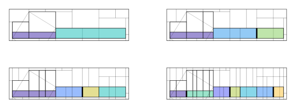
Figure 13: Successive greedy refinements for $\mathcal{R}_{A}^{\prime\prime}$.

The second key observation for dealing with the continuous phase space is that its geometrical measure (i.e., the Riemannian and not the SRB measure) determines a procedure for obtaining greedy refinements of any initial Markov partition (see Figures 9 and 11-13).

These greedy refinements are Markov by construction, and a subsequence of them is maximally uniform w/r/t the geometrical measure. Therefore, from the physical point of view, intermittent greedy refinements of an initial Markov partition are particularly natural. Indeed, their uniformity enables the proof of a finite value for $\lim\inf\beta$ for the cat map, where the limit inferior is taken over successive greedy refinements. Furthermore, considering greedy refinements for the geodesic flow also gives compelling numerical evidence that $\lim\inf\beta$ is not only finite but independent of global structure (see Figures 6 and 7).

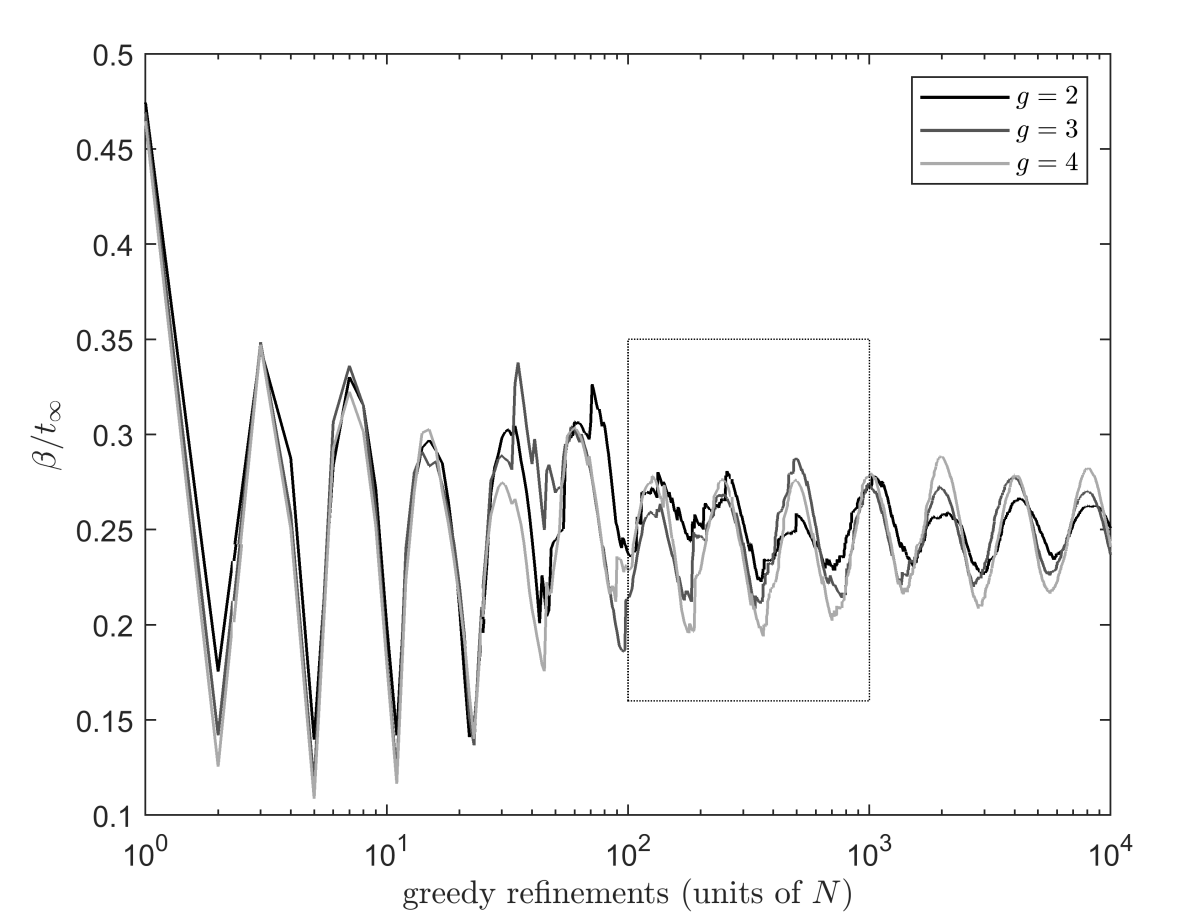
Figure 6: $\beta/t_{\infty}$ under successive greedy refinements of an initial Markov partition for a map isometrically topologically conjugate to a timing or Poincaré map of the geodesic flow on a compact surface of constant negative curvature with genus $g=2,3,4$. Note the logarithmic horizontal scale: here $N=8g-4$ is related to the number of rectangles in the initial partition. The inset box indicates axis limits for Figure 7.

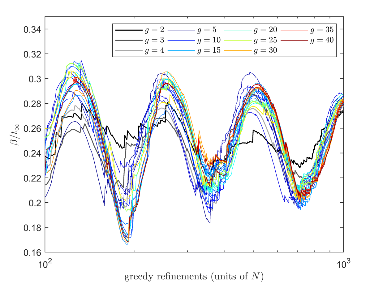
Figure 7: As in Figure 6 for $g=2,\dots,40$. Axis limits correspond to the inset box in Figure 6. The existence of a nontrivial limit inferior independent of $g$ is strongly suggested by such numerical results. Meanwhile, both the $L^{2}$ mixing time for sufficiently well-behaved observables and the inverse topological entropy turn out to be plausible genus-independent approximations for $t_{\infty}$.

We now turn to briefly describing how the preceding results bear on generic systems of interest in statistical physics. A product system formed from copies of the geodesic flow with canonically distributed initial conditions is just an ideal gas. By considering this gas as an environment and weakly coupling a subsystem to it, our focus shifts from a generalized microcanonical ensemble to the canonical ensemble, and a definition of a generic subsystem’s effective temperature in terms of that of its environment.

Such a procedure should often if not always give physically reasonable and self-consistent results, as we proceed to sketch. The results of amaricci2007analyticity and the general phenomenon of structural stability of Markov partitions for Anosov systems show that the effect on $\beta/t_{\infty}$ of coupling a Gaussian thermostat to the geodesic flow is analytic in the strength of the coupling. It is also reasonable to expect that $t_{\infty}$ will exhibit a similar regularity as a function of the coupling based on (e.g.) the stability of rapid mixing field2007stability . Many other examples are known in which well-behaved Anosov systems exhibit considerable stability of SRB measures and mixing times w/r/t perturbations, and it is reasonable to expect such behavior in general for physically relevant cases.

Taken together, these observations strongly suggest the existence and essential uniqueness of a physically preferred effective temperature and concomitant energy function intrinsic to generic mixing Anosov systems. Moreover, they suggest an avenue for extending Ruelle’s thermodynamical formalism Ruelle1 into a more comprehensive theory of statistical physics for nonequilibrium steady states obeying the chaotic hypothesis.

4.2 Background on Anosov systems

A smooth endomorphism $T$ of a Riemannian manifold (“phase space”) is an Anosov map if it is both

• uniformly hyperbolic, i.e. at every point $x$ there are transverse local stable and unstable surfaces on which points respectively converge and diverge exponentially at a rate independent of $x$; and

• invariant, i.e. the tangent spaces to these surfaces are mapped by the derivative of $T$ into the tangent spaces to the corresponding surfaces at $Tx\equiv T(x)$.

If the global stable and unstable surfaces of $T$ are dense, then $T$ is also said to be mixing. An Anosov flow is a continuous-time analogue of an Anosov map with a neutral surface transverse to the time evolution as schematically indicated in Figure 8. We refer to both Anosov maps and flows as Anosov systems.

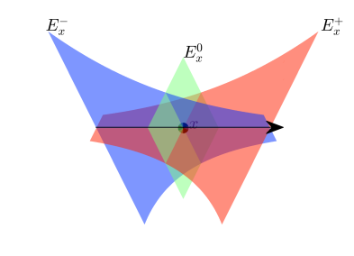
Figure 8: Schematic of an Anosov flow, with respective local stable, unstable, and neutral surfaces $E_{x}^{-}$, $E_{x}^{+}$, and $E_{x}^{0}$.

Anosov systems enjoy natural discretizations of their phase spaces. These discretizations, called Markov partitions, are particular configurations of rectangles. A rectangle $R$ is a subset of phase space such that the intersection of a local stable surface and a local unstable surface consists of a single point also in $R$: i.e., there is a local product structure compatible with $T$. A partition $\mathcal{R}=\{R_{j}\}_{j=1}^{n}$ of phase space into rectangles is Markov if (whenever these sets intersect) the images $TR_{j}$ stretch completely across $R_{k}$ in the unstable direction and $R_{k}$ stretches completely across $TR_{j}$ in the stable direction, as schematically indicated in Figure 9. The utility of the coarse-graining of phase space that Markov partitions provide is largely attributable to the fact that (via the theory of symbolic dynamics) they allow Anosov systems to be treated in much the same way as a spin system beck1995thermodynamics ; gallavotti1999statistical . This also highlights the relevance of both Anosov and spin systems as extremely generic (or as the chaotic hypothesis argues, completely generic) models for statistical physics.

Figure 9: Schematic of the action of an Anosov map on a rectangle that is part of a Markov partition. The image of the rectangle stretches precisely across other rectangles in the partition. If we suppose that the phase space measure corresponds to the Lebesgue measure of the rectangles, then a greedy refinement of the gray rectangle can be obtained by drawing a line at the inverse image of the intersection of the gray, red, and green rectangles. That is, a greedy refinement of a Markov partition $\mathcal{R}$ for an Anosov map $T$ starts by considering the forward image under $T$ of a rectangle $R_{j}\in\mathcal{R}$ with maximal geometrical/phase space (vs. physical/SRB) measure. The intersection of the boundary of $\mathcal{R}$ and $TR_{j}$ determines subrectangles of $T\mathcal{R}$ that in turn determine various refinements of $\mathcal{R}$ under $T^{-1}$. A greedy refinement has maximal entropy w/r/t the geometrical measure.

4.3 The cat map

The simplest example of an Anosov map is the Arnol’d-Avez cat map defined on the unit torus via $T_{A}x:=Ax\mod 1$, where $A=\left(\begin{smallmatrix}2&1\\ 1&1\end{smallmatrix}\right)$. The eigendecompositon of $A$ determines the stable and unstable directions. The eigenvalues are $\lambda_{\pm}=\phi^{\pm 2}$, where $\phi=\frac{1+\sqrt{5}}{2}$ is the golden ratio. The corresponding eigenvectors are $e_{-}=(s,-c)^{*}$ and $e_{+}=(c,s)^{*}$, where $c=1/\sqrt{3-\phi}$ and $s=\sqrt{1-c^{2}}$. Because these eigenvectors have irrational slopes, the stable and unstable surfaces are dense on the torus, so the cat map is mixing.

More generally, matrices in $GL(n,\mathbb{Z})$ with no eigenvalues in $S^{1}$ correspond to hyperbolic toral automorphisms which are also Anosov maps. In dimension $n=2$, rectangles for these maps are geometrically unions of parallelograms.

4.4 Markov partitions and greedy refinements

There are many Markov partitions for the cat map: Figure 10 shows three, respectively denoted $\mathcal{R}_{A}$, $\mathcal{R}^{\prime}_{A}$, and $\mathcal{R}^{\prime\prime}_{A}$.

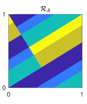
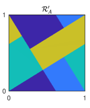
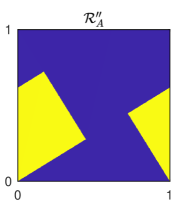
Figure 10: Three Markov partitions for the cat map.

A Markov partition $\mathcal{R}=\{R_{j}\}_{j=1}^{n}$ induces a probability distribution $p_{j}:=\mu(R_{j})$ inherited from the physical/SRB measure $\mu\equiv\mu_{SRB}$. For the cat map (or any other hyperbolic toral automorphism), this measure is just the Lebesgue measure.

For any two-dimensional hyperbolic toral automorphism $T$ (including the cat map), there is a remarkable fact (for details, see huntsman2010anosov ). Let $\mathcal{R}$ be a Markov partition and let $\mathcal{R}^{\vee}_{m}$ be a refinement of $\mathcal{R}$ obtained by taking connected components of intersections of rectangles in $T^{j}\mathcal{R}$ for $0\leq j\leq m$. Now as $m\rightarrow\infty$, $\beta/t_{\infty}=\lVert p\rVert\cdot\sqrt{\lVert\gamma\rVert^{2}+1}$ (which does not depend on $t_{\infty}$) converges to a finite nonzero value.

To see why any finite nonzero limit for $\beta/t_{\infty}$ is nontrivial, consider the following toy example. Define $\mathcal{Y}^{(0)}=[0,1]$ and form $\mathcal{Y}^{(m+1)}$ by subdividing each interval in $\mathcal{Y}^{(m)}$ into two subintervals of relative length $q$ and $1-q$. The corresponding partitions yield $\lim\beta/t_{\infty}=\infty$ unless $q=1/2$, in which case the limit is zero. Meanwhile, as we have mentioned, a naive discretization of the free particle/ideal gas has no obvious reasonable scaling limit.

The preceding results involving two-dimensional hyperbolic toral automorphisms indicate that while it might seem useful to consider $\beta=S_{n}\cdot t_{\infty}\lVert p\rVert\sqrt{\lVert\gamma\rVert^{2}+1}$ with $S_{n}=\sqrt{n}$ so that $\beta$ is independent of $n$, this is a mirage: we should actually require $S_{n}$ to be constant in $n$.

Now while detailed calculations establish that $\lim\beta/t_{\infty}$ depends on $\mathcal{R}$, and phase space (to say nothing of physical) measures of rectangles in $\mathcal{R}^{\vee}_{m}$ vary increasingly more as $m$ increases, there is a straightforward solution. We can construct greedy refinements of $\mathcal{R}$ that are more physically natural by maximizing the uniformity of phase space measures at each step of the refinement process. Even when the physical measure $\mu$ and phase space measure $\nu$ disagree, considering greedy refinements will tend to minimize $\beta$ and maximize entropy/minimize effective free energy. This is an indication of a generalized variational principle (in the sense of ergodic theory) that can yield a finite limit for $\beta$ even as the entropy of partitions diverges.

The construction of greedy refinements goes as follows. For a rectangle $R_{j}\in\mathcal{R}$ with maximal phase space measure $\nu(R_{j})$, the intersection of $TR_{j}$ with rectangles in $\mathcal{R}$ determines subrectangles of $T\mathcal{R}$ that in turn determine various refinements of $\mathcal{R}$ under $T^{-1}$. We call such a refinement of maximal entropy (with respect to $\nu$) greedy. In general, greedy refinements are not unique, though subsequences of them (corresponding to the result of greedily refining all of the rectangles of maximal $\nu$-measure at a time) will be. Figures 11-12 illustrate greedy refinements for the Markov partitions in Figure 10.

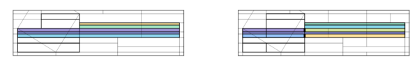
Figure 11: (L) In black, we show the Markov partition $\mathcal{R}_{A}$ from Figure 10 in eigencoordinates, with both the unit square and translates in gray. The forward image $T\mathcal{R}_{A}$ is shown in color. There are two rectangles of maximal $\nu$-measure: the third and fifth from the top. (R) Greedily refining each of the two rectangles of maximal $\nu$-measure by taking intersections as demarcated by bold black lines.

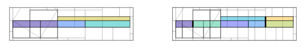
Figure 12: (L) As in Figure 11, but for $\mathcal{R}_{A}^{\prime}$. (R) The result of two greedy refinements. Note that the result of a round of greedy refinements is not unique, though the value of the resulting $\nu$-entropy is.

These greedy refinements stabilize the measures of rectangles. Detailed calculations show that certain greedy refinements of both $\mathcal{R}_{A}$ and $\mathcal{R}_{A}^{\prime}$ contain $L_{m+1}$ and $L_{m+2}$ rectangles of relative measure $1$ and $\phi$, respectively. Here the Lucas numbers are defined via $L_{m+2}=L_{m+1}+L_{m}$ with $L_{1}=1$, $L_{2}=3$. However, $\mathcal{R}_{A}^{\prime}$ behaves differently, with maximally uniform greedy refinements containing $L_{m-1}$ and $L_{m}$ rectangles of relative measure $1$ and $\phi$, respectively. Nevertheless, in each of these three cases there is a common limit $\lim\beta/t_{\infty}\approx 0.2393$, which is probably minimal/universal for the cat map. In any event, while the detailed measures of greedy refinements depend on an initial Markov partition, we can always consider an extremum over Markov partitions with decreasing size to obtain (by construction) a unique physically natural result.

4.5 The geodesic flow on a surface of constant negative curvature

The geodesic flow on a surface of constant negative curvature is the archetypal Anosov flow anosov1969geodesic ; klingenberg1974riemannian . It corresponds to the free particle Hamiltonian collet1984perturbations $\mathcal{H}=\frac{1}{2m}\sum_{jk}g^{jk}P_{j}P_{k}$, where we use typical notation for the inverse of the metric tensor and for momenta on the cotangent bundle. For a surface of constant negative curvature, the geodesic flow is mixing, and as we shall see the effective temperature is apparently insensitive to the surface genus.

We briefly recall the details of the geodesic flow in the Poincaré disk model following adler1991geodesic (see also bowen1979markov ; gutzwiller1990chaos ). The differential arclength is $ds=dr/(1-r^{2})$, and geodesics correspond to circular arcs intersecting $S^{1}$ at right angles (see Figure 14). A surface of constant negative curvature can be obtained by identifying pairs of edges $s_{j}$ of a hyperbolic polygon via maps $T_{j}(s_{j})=s_{\sigma(j)}^{-1}$. Here $s_{j}^{-1}$ denotes the orientation reversal of $s_{j}$, and the pairing $\sigma$ is defined along the lines shown for the genus 2 case of Figure 14. If there are $8g-4$ edges, this procedure yields a surface of genus $g$. Finally, the Hamiltonian is $\mathcal{H}=(1-r^{2})^{2}\cdot P^{2}/2m$.

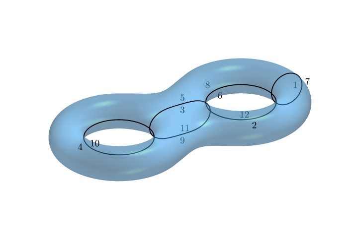
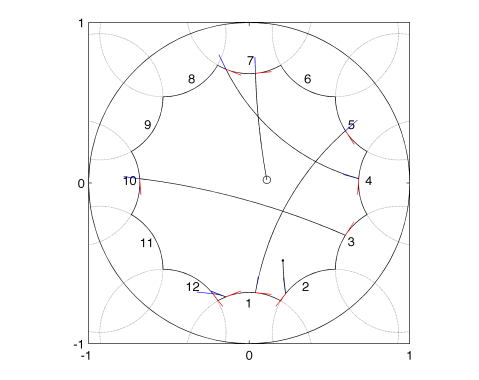
Figure 14: (L) A surface with genus $g=2$. For $g\geq 2$ there are surfaces of constant (or more generally global) negative curvature and whose geodesic flows are mixing (hence also ergodic). The construction of Adler and Flatto provides examples. For $g=2$, the corresponding 12-gon can be recovered by cutting along the indicated paths. Incrementing $g$ by adding a handle also requires adding two more geodesic loops; one of the new loops and one of the old loops are separated into two arcs by their intersections with neighboring loops, and cutting along these arcs yields eight new edges. This construction underlies the pairing of edges of $F$, which is indicated explicitly here for $g=2$. (R) Model of the geodesic flow for genus $g=2$ with 12-gon labels as indicated in the left panel. A sample trajectory is also indicated, with initial condition given by the open marker close to the center of the figure. Blue and red segments respectively indicate tangent directions to the flow and 12-gon at the latter’s boundary.

We can construct a Poincaré or timing map and associated Markov partition for the geodesic flow. The first step is to instantiate edge pairing maps $T_{j}$ en route to a map $T_{R}$ which will be the composition of the Poincaré map and an isometry. Then, we perform numerical calculations using the map $T_{R}$ and a Markov partition $\mathcal{R}$ for it. The advantage of this construction is that “rectangles are rectangles,” even though $T_{R}$ is nonlinear. For example, Figure 15 shows $\mathcal{R}$, $T_{R}\mathcal{R}$, and $T_{R}^{2}\mathcal{R}$ for the genus $g=2$ case. From these Markov partitions, we obtain refinements $\mathcal{R}_{m}^{\lor}$ by intersecting rectangles in $T^{0}_{R}\mathcal{R},\dots,T^{m}_{R}\mathcal{R}$.

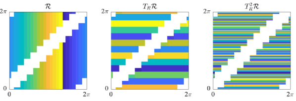
Figure 15: The Markov partitions $\mathcal{R}$, $T_{R}\mathcal{R}$, and $T_{R}^{2}\mathcal{R}$ for the $g=2$ case. Note that rectangles become disconnected for $T_{R}^{2}\mathcal{R}$.

Although as with hyperbolic toral automorphisms we have $\mu=\nu$ in this situation, this common measure is substantially more complicated than Lebesgue measure, viz.

$$\mu([x_{1},x_{2}]\times[y_{1},y_{2}])=\int_{y_{1}}^{y_{2}}\int_{x_{1}}^{x_{2}}\frac{\lvert dx\ dy\rvert}{\lvert e^{ix}-e^{iy}\rvert^{2}}.$$

Consequently, the numerical computation of measures of rectangles in refinements of $\mathcal{R}$ is nontrivial. It turns out that $\beta/t_{\infty}$ diverges nearly exponentially for $\mathcal{R}_{m}^{\lor}$, whereas for the cat map $\beta/t_{\infty}$ provably converges due to linearity.

However, for greedy refinements there is strong numerical evidence that $\lim\inf\beta$ is well-defined, nonzero, finite, and independent of genus $g$ (see Figures 6 and 7). This is due not only to the convergence of $\beta/t_{\infty}$, but also to the fact that the $L^{2}$ mixing time of the geodesic flow is $1/2$ for $g$ arbitrary.

4.6 Conclusion

As archetypal Anosov systems, the cat map and the geodesic flow on a surface of constant negative curvature are deeply relevant to statistical physics. These and other Anosov systems exhibit Markovian symbolic dynamics that highlights both chaotic properties and correspondences with spin systems. The chaotic hypothesis seizes on these features to argue that Anosov systems are themselves archetypal model statistical-physical systems. For example, taking copies of the geodesic flow of §4.5 with different initial conditions yields an ideal gas, and weakly coupling to this yields a thermometer.

As foreshadowed in §4.1, the results of amaricci2007analyticity and structural stability of Markov partitions for Anosov systems indicate that such a coupling leads to effects that vary analytically with the coupling strength. Moreover, the stability of rapid mixing field2007stability gives at least one reason to expect that $t_{\infty}$ will also behave nicely as a function of coupling strength. SRB measures and mixing times for Anosov systems are well-behaved in many examples, and it is reasonable to expect this for physically relevant examples.

While of course Markov structures (i.e., partitions or sections) are not unique, it is nevertheless evident that phenomena which hold for any Markov structure on an Anosov system are likely to be of relevance to statistical physics. In this vein, the observed limiting behavior of $\beta/t_{\infty}$ as calculated on greedy partitions for both two-dimensional hyperbolic toral automorphisms and the geodesic flow is remarkable. While rigorously elaborating on this behavior would seem to require the development of new and nontrivial mathematics, it nevertheless appears to be generic.

Of particular importance are the implications that the evidence of this limiting behavior has for a proposed general theory of nonequilibrium steady states.

We have argued here for a comprehensive framework for nonequilibrium statistical physics that simultaneously incorporates and extends the formalism originally introduced by Ruelle and subsequently refined by Gallavotti, Cohen and others. The framework has as its goal a broad theory of nonequilibrium statistical physics that is truly intrinsic: i.e., that provides information about physical observables simply in terms of raw temporal information about the dynamics.

One reason to consider a proposal of the sort described here, in which the concept of (effective) temperature plays the central role, is because there is no generally accepted physical definition of entropy for non-equilibrium steady states. We hope that the ideas discussed here will serve to elicit fruitful investigations into the fundamental nature of stationary physical systems far from equilibrium.

- (1) C. Amey, J. Machta, Physical Review E 97(3), 033301 (2018)
- (2) K. Binder, D.W. Heermann, Monte Carlo Simulation in Statistical Physics: An Introduction (Springer, 2019)
- (3) G. Gallavotti, E.G.D. Cohen, Journal of Statistical Physics 80(5-6), 931 (1995)
- (4) G. Gallavotti, Statistical Mechanics: A Short Treatise (Springer, 1999)
- (5) B. Durhuus, J. Fröhlich, Communications in Mathematical Physics 75(2), 103 (1980)
- (6) M. Richey, The American Mathematical Monthly 117(5), 383 (2010)
- (7) S. Brooks, A. Gelman, G. Jones, X.L. Meng, Handbook of Markov Chain Monte Carlo (CRC, 2011)
- (8) R.M. Neal, arXiv preprint arXiv:1101.0387 (2011)
- (9) J.F. Delmas, B. Jourdain, Journal of Applied Probability 46(4), 938 (2009)
- (10) S. Huntsman, in International Conference on Artificial Intelligence and Statistics (2020), pp. 2841–2851
- (11) P. Brémaud, Markov Chains: Gibbs Fields, Monte Carlo Simulation, and Queues (Springer, 1999)
- (12) P.H. Peskun, Biometrika 60(3), 607 (1973)
- (13) A.L. Onishchik, E.B. Vinberg, Lie Groups and Algebraic Groups (Springer, 1990)
- (14) A. Kirillov, An Introduction to Lie Groups and Lie Algebras (Cambridge, 2008)
- (15) C.P. Robert, V. Elvira, N. Tawn, C. Wu, Wiley Interdisciplinary Reviews: Computational Statistics 10(5), e1435 (2018)
- (16) J.S. Liu, F. Liang, W.H. Wong, Journal of the American Statistical Association 95(449), 121 (2000)
- (17) L. Martino, Digital Signal Processing 75, 134 (2018)
- (18) L. Martino, D. Luengo, J. Míguez, Independent Random Sampling Methods (Springer, 2018)
- (19) B. Calderhead, Proceedings of the National Academy of Sciences 111(49), 17408 (2014)
- (20) M. Niepert, in Proceedings of the Twenty-Eighth Conference on Uncertainty in Artificial Intelligence (2012), pp. 624–633
- (21) M. Niepert, in Proceedings of the Second Statistical Relational AI Workshop (2012)
- (22) H.H. Bui, T.N. Huynh, S. Riedel, in Proceedings of the Twenty-Ninth Conference on Uncertainty in Artificial Intelligence (2013), pp. 132–141
- (23) R. Shariff, A. György, C. Szepesvári, in Artificial Intelligence and Statistics (2015), pp. 866–874
- (24) G.V.d. Broeck, M. Niepert, in Proceedings of the Twenty-Ninth AAAI Conference on Artificial Intelligence (2015), pp. 3599–3605
- (25) A. Anand, A. Grover, M. Mausam, P. Singla, in Proceedings of the Twenty-Fifth International Joint Conference on Artificial Intelligence (2016), pp. 3560–3568
- (26) J.S. Liu, Y.N. Wu, Journal of the American Statistical Association 94(448), 1264 (1999)
- (27) J.S. Liu, C. Sabatti, Biometrika 87(2), 353 (2000)
- (28) L. Saloff-Coste, Notices of the AMS 48(9), 968 (2001)
- (29) T. Ceccherini-Silberstein, F. Scarabotti, F. Tolli, Harmonic Analysis on Finite Groups (Cambridge, 2008)
- (30) J.G. Sumner, J. Fernández-Sánchez, P.D. Jarvis, Journal of Theoretical Biology 298, 16 (2012)
- (31) H. Suwa, S. Todo, Physical Review Letters 105(12), 120603 (2010)
- (32) T.L. Chen, C.R. Hwang, Statistics & Probability Letters 83(9), 1956 (2013)
- (33) J. Bierkens, Statistics and Computing 26(6), 1213 (2016)
- (34) K. Takahashi, M. Ohzeki, Physical Review E 93(1), 012129 (2016)
- (35) A. Frigessi, C.R. Hwang, L. Younes, et al., The Annals of Applied Probability 2(3), 610 (1992)
- (36) L. Pollet, S.M. Rombouts, K. Van Houcke, K. Heyde, Physical Review E 70(5), 056705 (2004)
- (37) T.L. Chen, W.K. Chen, C.R. Hwang, H.M. Pai, SIAM Journal on Control and Optimization 50(5), 2743 (2012)
- (38) S.J. Wu, M.T. Chu, Linear Algebra and its Applications 487, 184 (2015)
- (39) L.J. Huang, Y.T. Liao, T.L. Chen, C.R. Hwang, SIAM Journal on Control and Optimization 56(4), 2977 (2018)
- (40) J.E. Johnson, Journal of Mathematical Physics 26(2), 252 (1985)
- (41) D.G. Poole, The American Mathematical Monthly 102(9), 798 (1995)
- (42) A. Boukas, P. Feinsilver, A. Fellouris, Random Operators and Stochastic Equations 23(4), 209 (2015)
- (43) M. Guerra, A. Sarychev, arXiv preprint arXiv:1805.07299 (2018)
- (44) J. Hilgert, K.H. Neeb, Lie Semigroups and their Applications (Springer, 1993)
- (45) C. Dawson, M. Nielsen, Quantum Information and Computation 6(1), 81 (2006)
- (46) F. Casas, A. Murua, M. Nadinic, Computer Physics Communications 183(11), 2386 (2012)
- (47) R.A. Horn, C.R. Johnson, Matrix Analysis, 2nd edn. (Cambridge, 2012)
- (48) D.J. Earl, M.W. Deem, Physical Chemistry Chemical Physics 7(23), 3910 (2005)
- (49) E. Bolthausen, A. Bovier, Spin Glasses (Springer, 2007)
- (50) D. Panchenko, Journal of Statistical Physics 149(2), 362 (2012)
- (51) P.R. Conrad, A.D. Davis, Y.M. Marzouk, N.S. Pillai, A. Smith, SIAM/ASA Journal on Uncertainty Quantification 6(1), 339 (2018)
- (52) M. Dashti, A.M. Stuart, in Handbook of Uncertainty Quantification, ed. by R. Ghanem, D. Higdon, H. Owhadi (Springer, 2017)
- (53) L. Martino, F. Leisen, J. Corander, arXiv preprint arXiv:1409.0051 (2014)
- (54) L. Khachiyan, in Advances in Convex Analysis and Global Optimization (Springer, 2001), pp. 105–118
- (55) L. Khachiyan, E. Boros, K. Borys, K. Elbassioni, V. Gurvich, Discrete & Computational Geometry 39(1), 174 (2008)
- (56) D.K. Faddeev, Uspekhi Matematicheskikh Nauk 11(1), 227 (1956)
- (57) J.C. Baez, T. Fritz, T. Leinster, Entropy 13(11), 1945 (2011)
- (58) G. Gallavotti, The European Physical Journal B 61(1), 1 (2008)
- (59) A.Q. Tool, Journal of the American Ceramic Society 29(9), 240 (1946)
- (60) T.M. Nieuwenhuizen, Physical Review Letters 80(25), 5580 (1998)
- (61) L. Leuzzi, T.M. Nieuwenhuizen, Thermodynamics of the Glassy State (Taylor & Francis, 2007)
- (62) L.F. Cugliandolo, Journal of Physics A: Mathematical and Theoretical 44(48), 483001 (2011)
- (63) A. Puglisi, A. Sarracino, A. Vulpiani, Physics Reports 709, 1 (2017)
- (64) H.H. Rugh, Physical Review Letters 78(5), 772 (1997)
- (65) H.H. Rugh, Journal of Physics A: Mathematical and General 31(38), 7761 (1998)
- (66) S. Huntsman, arXiv preprint arXiv:1009.2127 (2010)
- (67) D. Ford, arXiv preprint cond-mat/0510291 (2005)
- (68) D. Ford, S. Huntsman, Physica A: Statistical Mechanics and its Applications 365(1), 34 (2006)
- (69) S. Braun, J.P. Ronzheimer, M. Schreiber, S.S. Hodgman, T. Rom, I. Bloch, U. Schneider, Science 339(6115), 52 (2013)
- (70) J. Dunkel, S. Hilbert, Nature Physics 10(1), 67 (2014)
- (71) D. Frenkel, P.B. Warren, American Journal of Physics 83(2), 163 (2015)
- (72) E.T. Jaynes, Physical Review 106(4), 620 (1957)
- (73) E. Buckingham, Physical Review 4(4), 345 (1914)
- (74) G. Barenblatt, Scaling (Cambridge, 2003)
- (75) H. Goldstein, C. Poole, J. Safko, Classical Mechanics, 3rd edn. (Addison-Wesley, 2001)
- (76) G. Gallavotti, E. Verboven, Il Nuovo Cimento B (1971-1996) 28(1), 274 (1975)
- (77) G. Parisi, Statistical Field Theory (Perseus, 1998)
- (78) O. Bratteli, D.W. Robinson, Operator Algebras and Quantum Statistical Mechanics: Volume 1: C*-and W*-Algebras. Symmetry Groups. Decomposition of States (Springer, 2012)
- (79) A. Connes, C. Rovelli, Classical and Quantum Gravity 11(12), 2899 (1994)
- (80) P. Martinetti, C. Rovelli, Classical and Quantum Gravity 20(22), 4919 (2003)
- (81) C. Rovelli, Classical and Quantum Gravity 10(8), 1567 (1993)
- (82) Y. Tian, Journal of High Energy Physics 2005(06), 045 (2005)
- (83) C. Rovelli, M. Smerlak, Classical and Quantum Gravity 28(7), 075007 (2011)
- (84) H. Reiss, Methods of Thermodynamics (Dover, 1997)
- (85) Y. Choquet-Bruhat, C. DeWitt-Morette, M. Dillard-Bleick, Analysis, Manifolds, and Physics (North-Holland, 1977)
- (86) J.R. Chazottes, B. Fernandez, Dynamics of Coupled Map Lattices and of Related Spatially Extended Systems (Springer, 2005)
- (87) P. Collet, H. Epstein, G. Gallavotti, Communications in Mathematical Physics 95(1), 61 (1984)
- (88) B. Saussol, Reviews in Mathematical Physics 21(08), 949 (2009)
- (89) J. Barrera, B. Lachaud, B. Ycart, Stochastic Processes and their Applications 116(10), 1433 (2006)
- (90) G. Schwarz, Reviews of Modern Physics 40(1), 206 (1968)
- (91) E.T. Jaynes, in Maximum-Entropy and Bayesian Methods, ed. by G. Erickson, P. Neudorfer, C. Smith (Springer, 1992)
- (92) A. Katok, B. Hasselblatt, Introduction to the Modern Theory of Dynamical Systems, vol. 54 (Cambridge, 1997)
- (93) D. Richeson, J. Wiseman, Topology and its Applications 156(2), 251 (2008)
- (94) S. Huntsman, arXiv preprint arXiv:0904.3881 (2009)
- (95) M. Burgess, Physical Review E 62(2), 1738 (2000)
- (96) G. Gentile, Forum Mathematicum 10(1), 89 (1998)
- (97) D. Ford, arXiv preprint cond-mat/0601387 (2006)
- (98) S. Boccaletti, J. Kurths, G. Osipov, D. Valladares, C. Zhou, Physics Reports 366(1-2), 1 (2002)
- (99) J.A. Acebrón, L.L. Bonilla, C.J.P. Vicente, F. Ritort, R. Spigler, Reviews of Modern Physics 77(1), 137 (2005)
- (100) F. Dorfler, F. Bullo, SIAM Journal on Control and Optimization 50(3), 1616 (2012)
- (101) E. Cohen, Physica A: Statistical Mechanics and its Applications 305(1-2), 19 (2002)
- (102) E. Cohen, in Boltzmann’s Legacy, ed. by G. Gallavotti, W. Reiter, J. Yngvason (EMS, 2008)
- (103) H. Chang, Inventing Temperature (Oxford, 2004)
- (104) R. Bowen, Springer Lecture Notes in Math 470, 78 (1975)
- (105) N. Chernov, in Handbook of Dynamical Systems, vol. 1A, ed. by A. Katok, B. Hasselblatt (North-Holland, 2002), pp. 321–407
- (106) D.Q. Jiang, D. Jiang, M. Qian, Mathematical Theory of Nonequilibrium Steady States (Springer, 2004)
- (107) L.S. Young, Journal of Statistical Physics 108(5-6), 733 (2002)
- (108) D. Dolgopyat, Annals of Mathematics 147(2), 357 (1998)
- (109) C. Liverani, Annals of Mathematics pp. 1275–1312 (2004)
- (110) O. Butterley, K. War, Journal of the European Mathematical Society 22(7), 2253 (2020)
- (111) M. Tsujii, Z. Zhang, arXiv preprint arXiv:2006.04293 (2020)
- (112) A. Wilkinson, in Encyclopedia of Complexity and Systems Science, ed. by R.A. Meyers, B. Kra (Springer, 2009)
- (113) A. Amaricci, F. Bonetto, P. Falco, Journal of Mathematical Physics 48(7), 072701 (2007)
- (114) D.J. Evans, S. Sarman, Physical Review E 48(1), 65 (1993)
- (115) F. Bonetto, G. Gallavotti, A. Giuliani, F. Zamponi, Journal of Statistical Physics 123(1), 39 (2006)
- (116) G. Gallavotti, Chaos: An Interdisciplinary Journal of Nonlinear Science 19(1), 013101 (2009)
- (117) G. Gallavotti, E. Presutti, Journal of Mathematical Physics 51(1), 015202 (2010)
- (118) G. Gallavotti, E. Presutti, Journal of Mathematical Physics 51(5), 053303 (2010)
- (119) M. Field, I. Melbourne, A. Török, Annals of Mathematics pp. 269–291 (2007)
- (120) D. Ruelle, Thermodynamic Formalism (Addison-Wesley, 1978)
- (121) C. Beck, F. Schögl, Thermodynamics of Chaotic Systems: An Introduction (Cambridge, 1995)
- (122) D.V. Anosov, Geodesic Flows on Closed Riemann Manifolds with Negative Curvature (American Mathematical Society, 1969)
- (123) W. Klingenberg, Annals of Mathematics pp. 1–13 (1974)
- (124) R. Adler, L. Flatto, Bulletin (New Series) of the American Mathematical Society 25(2), 229 (1991)
- (125) R. Bowen, C. Series, Publications Mathématiques de l’Institut des Hautes Études Scientifiques 50(1), 153 (1979)
- (126) M. Gutzwiller, Chaos in Classical and Quantum Mechanics (Springer, 1990)