Invited: Drug Discovery Approaches using
Quantum Machine Learning

Abstract

Traditional drug discovery pipeline takes several years and cost billions of dollars. Deep generative and discriminative models are widely adopted to assist in drug development. Classical machines cannot efficiently produce atypical patterns of quantum computers which might improve the training quality of learning tasks. We propose a suite of quantum machine learning techniques e.g., generative adversarial network (GAN), convolutional neural network (CNN) and variational auto-encoder (VAE) to generate small drug molecules, classify binding pockets in proteins, and generate large drug molecules, respectively.

I Introduction

Modern pharmaceutical research uses automated high-throughput screening technologies to discover new biologically target-binding compounds, but the development of a new drug is still a long and expensive process. Computational molecular docking offers an efficient and inexpensive way to identify target-binding compounds and to estimate the binding affinity between compounds and targets. The success rate of virtual drug screening is dictated mainly by 1) the docking accuracy and 2) the comprehensiveness of the compound library used for screening. The docking accuracy of a docking software is decided by its ability to sample compound and target conformations [1], as well as the accuracy of its scoring method [2]. Significant strides have been made to enhance the sampling and scoring procedures [3] and utilizing massive protein–ligand complex structures to train the scoring function. Numerous docking methods (see Fig. 1(a) for docking engine mechanism) have been proposed and evaluated, such as Glide [4], MedusaDock [5, 6], AutoDock Vina [7].

Quantum computing can offer unique advantages over classical computing in many fields, such as chemistry simulation, machine learning, and optimization. Quantum GAN is one of the main applications of near-term quantum computers due to its strong expressive power in learning data distributions even with much less parameters compared to classical GANs. However, quantum neural network is still at its nascent stage due to qubit constraints on noisy quantum computers. Considering the specific task of drug discovery, we explore potential quantum advantages for both generative and predictive models due to the following reasons: 1) Gate parameter exploration in Hilbert space is different from neural network parameter exploration. Exponentially growing Hilbert space offers chance to explore certain chemical regions that are not accessible to classical GANs. 2) Given a chemical region abundant of molecules, the inherent probabilistic nature of quantum systems helps generate more diverse and novel (though also less valid) molecules surrounding that region.

This paper presents three new Quantum Machine Learning (QML) techniques for drug discovery namely, a hybrid (i) quantum GAN to learn the patterns in molecular dataset and generate small drug-like molecules, (ii) quantum classifier for protein pocket classification, (iii) quantum VAE to generate a probabilistic cloud of molecules to screen a molecular dataset. In the remaining paper, we cover the background on drug discovery, quantum computing, and QML in Section II, discuss three QML applications in drug discovery and development in Section III, and draw conclusion in Section IV.

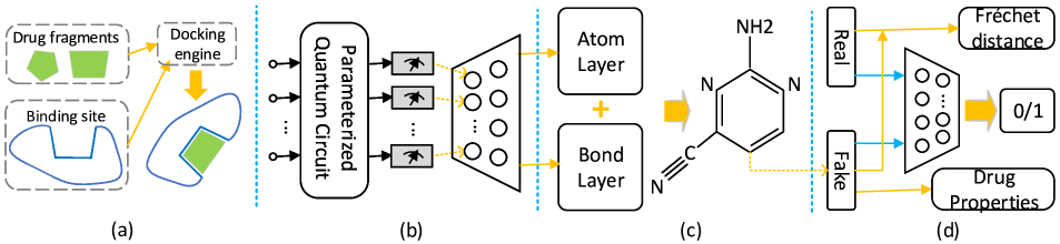
Figure 1: (a) Only generated molecules that have high affinity towards the receptor binding sites are considered as valid; (b) quantum stage and classical stage separated by blue dotted line; (c) application of atom layer and bond layer for generating synthetic molecular graphs; (d) a batch of real molecules from training dataset (QM9 in this case) and a batch of synthetic molecules generated from (c) are fed into classical discriminator for real/synthetic prediction and FD score calculation, and drug properties for synthetic molecules are evaluated using RDKit [8, 9].

II Background

Drug discovery problem: Historically, drugs have been discovered incidentally, such as penicillin. Nowadays, chemical compounds are selected from databases for extensive preclinical studies based on druglikeness and synthesizability as measured by heuristics. These compounds are screened for biological activity with a variety of protein assays. Naturally occurring bioactive compounds may be identified from plant and animal samples from diverse ecosystems. Medicinal chemists may further optimize selected compounds to maximize binding affinities and synthesizability. Compounds which show promise in the preclinical setting are then screened in cell lines and animals before making it to human trials.

Classical approaches to drug discovery: Compounds are typically experimentally screened for activity against potential receptors in vitro by quantitatively measuring the binding of the compound to the receptor. Computational approaches determine characteristics of receptors and compounds which facilitate binding. The most accurate predictions obtainable come from density functional theory, however these calculations are limited to small molecules and receptor fragments.

As an approximation to the quantum mechanical properties of compounds and receptors, a variety of chemical fingerprint algorithms have been developed. Given a molecule and the receptor it binds, fingerprint similarity can be used to screen a library of molecules of other compounds which may be active against the receptor. Recently, machine learning has become a promising candidate for virtual high-throughput screening pipelines. The MolGAN model uses a generative adversarial network (GAN) to learn and generate drug-like molecules based on the QM9 dataset [10, 11]. To improve the quality of generated compounds and stabilize the GAN training, a reward network based on chemical validity (RDKit[8]) is used.

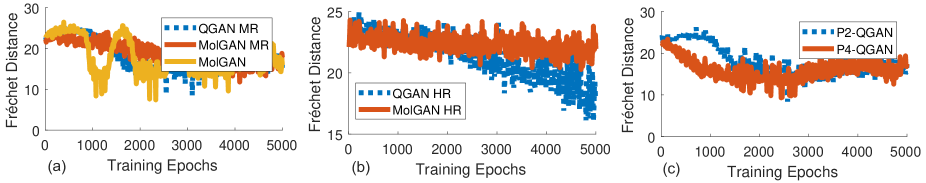
Figure 2: Training comparison among GAN flavors: (a) Fréchet distances for MolGAN, moderately reduced (14.93%) MolGAN and QGAN-HG; (b) Fréchet distances for highly reduced (1.97%) MolGAN and QGAN-HG; (c) learning curves for patched QGAN-HG with two sub-circuits and four sub-circuits [9].

Quantum computing and QML: Quantum computing uses quantum phenomena such as, superposition and entanglement to perform computation. Qubits are the building blocks of quantum computers which is analogous to classical bits however, a qubit can be in a superposition state i.e., a combination of 0 and 1 at the same time. Quantum gates (e.g., 1-qubit Pauli-X ($\sigma_{x}$) gate, 2-qubit CNOT gate, etc.) modulate the state of qubits and thus, perform computation. QML involves parameter optimization of parameterized quantum circuits to obtain a desired input-output relationship. Although none of the existing QML models have a provable performance guarantee over the classical models, several works claim that QML models have high expressibility [12].

III QML for drug discovery

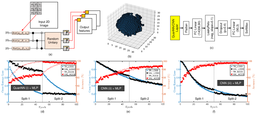
Figure 3: (a) A toy Quanvolution operation on a 2D image segment to generate output feature maps using random quantum circuit, (b) a single channel of a sample protein pocket in the TOUGH-C1 dataset, (c) deep learning pipeline used in the case-study, (d) performance of QuanvNN (no trainable parameters) + MLP, (e) CNN (no trainable parameters) + MLP, and (f) CNN (with trainable parameters) + MLP.

III-A Approach-1: QGAN-HG

Generative learning with graph-structured molecules is invariant to the orderings of atoms [10] and automates the navigation to a chemical region abundant in desired molecules. The proposed qubit-efficient quantum GAN with hybrid generator and classical discriminator (QGAN-HG) [9] efficiently learns molecule distributions based on classical MolGAN (Fig. 1). We also examine the patched circuit idea [13] by comparing to the original single large generator circuit implementation using metric of Fréchet distance and drug property scores. Quantum GAN with hybrid generator (QGAN-HG) is composed of a parameterized circuit to get a feature vector of qubit size dimension, and a classical deep neural network to output an atom vector and a bond matrix for the graph representation of drug molecules. Another patched quantum GAN with hybrid generator (P-QGAN-HG) is considered as the variation of QGAN-HG where the quantum circuit is formed by concatenating few quantum sub-circuits. The variational quantum circuit consists of 3 stages, namely initialization, entanglement and measurement stages. Classical stage of hybrid generator is a standard neural network with input layer receiving the feature vector of expectation values. Note that, 85.07% and 98.03% of generator parameters are respectively cropped from classical GAN [10] to demonstrate the strong expressive power of quantum circuits. We also implement two enhanced QGAN-HG variants with $L=2$ and $N=10$.

We conduct the experiments with QM9 [11] dataset. Generated molecule distribution is approximately created by generating a batch of molecules, and real one is approximately formed by randomly sampling the same number of molecules from QM9. Generated drug quality is evaluated using metrics such as druglikeness, solubility and synthesizability using RDKit [8]. The learning rate is set to 0.0001 and starts decaying uniformly at a factor of $1/2000$ after 3000 epochs. Total training epoch is set with 5000, and early stopping based on Fréchet distance is applied under model collapse.

Fig. 2(a-b) compares the performance between MolGAN and QGAN-HG for moderately and highly reduced architectures. All mechanisms can reach a reasonably good training point within 5000 epochs, however, moderately reduced MolGAN takes around 4000 iterations while original MolGAN and QGAN-HG take $\approx$2500. MolGAN with highly reduced architecture can hardly be learned though a slight downward trend is observed. Quantum circuit involves only 15 gate parameters illustrating the strong expressive power of variational quantum circuits. We examine two patched QGAN-HG variations, i.e., P2-QGAN with two sub-circuits (each has 4 qubits and 7 gate parameters) and P4-QGAN with four sub-circuits (each has 2 qubits and 3 parameters). Surprisingly, the learning quality of the patched QGANs (with even less gate parameters) are comparable to QGAN with an integral circuit (Fig. 2(a, c)).

III-B Approach-2: Image based search

Most of the deep learning solutions for drug discovery use 3D grid representation of the molecular structures. Each grid-point is commonly referred to as voxels. For example, voxel representation of ligand-binding protein pockets are used as inputs to a convolutional deep neural network (CNN) in [14] to classify the pockets in one of 3 groups: nucleotide-binding or heme-binding or others. In this section, we pick the pocket classification problem in [14] as our test-case and the quanvolutional neural networks presented in [15] to gauge the efficacy of QML models in drug development pipelines.

Quanvolutional Neural Networks: A quantum analogous of the conventional CNN for image recognition tasks has been proposed [15] (referred as Quanvolutional Neural Networks (QuanNN)) where filters are replaced by quantum circuits. Each filter takes a segment of the input image and encode the data as a quantum state with suitable encoding scheme (e.g., angle or amplitude encoding). Later, a random (/structured) quantum circuit transforms the state and the output is measured repeatedly to generate a feature map. Similar to CNN, the filter moves across the entire image in finite steps to generate new feature maps for the entire image (Fig. 3(a)).

Dataset: The TOUGH-C1 dataset [14] used for this work contains 4095 samples. Each sample is represented by a 14x32x32x32 tensor (14 channels). The dataset contains 1553 nucleotide-binding, 596 heme-binding, and 1946 other type of protein pockets. A single channel of a protein pocket in the dataset is shown in Fig. 3(b).

Deep Learning Pipeline: We have used 3 deep learning pipelines with QuanNN, CNN, and multi-layer perceptrons (MLP): (i) single-layer QuanNN (no trainable parameters) + MLP, (ii) single-layer CNN (no trainable parameters) + MLP, and (iii) single-layer CNN + MLP (Fig. 3(c)). Cross entropy is used as the loss function for all these networks. The QuanNN and CNN layers both produce 14336 dimensional representation of the input 3D pocket grids. For the CNN, we use 28 output channels with kernel-size = 4 and, and stride = 4 which produces 8x8x8x28 (14336) dimensional output features. For the QuanNN, we use a 4-qubit quantum circuit as the filter and take the Pauli-Z expectation values of the qubits (4) as output features. The quantum circuit consists of ’StronglyEntanglingLayers’ from Pennylane [16] that encodes the input classical data as rotation angles at different qubits followed by all-qubit entanglement with CNOT operations. A random 4-qubit quantum circuit is placed in front of the encoding block for random transformation of the quantum state using ’RandomLayers’ class in the Pennylane framework. The quantum circuit takes a 4x4x4 dimensional tensor block from 2 channels at a time (2x4x4x4 dimensional input). For 14x32x32x32 dimensional 3D grids (14 channels), it produces 7x8x8x8x4 (14336) output features.

Metrics: We model and train all three networks using PyTorch and Pennylane libraries under identical configurations. We perform stratified 2-fold cross-validation training of the models for 50 epochs/split with a batch-size of 32 and learning-rate of $e^{-5}$. We use the cross-entropy loss and classification accuracy as the metrics for performance.

Comparison: In our simulations, (i) outperformed (ii) by a significant margin (Fig. 3(d)&(e)). At the end of the training, (i) achieved $\approx$55% lower cross-entropy loss, and $\approx$17% higher accuracy over (ii) for the training set. For the validation set, the loss was $\approx$57% lower, and accuracy was $\approx$14% higher. However, compared to (iii) (Fig. 3(f)), (i) showed $\approx$11% higher loss but $\approx$2% higher accuracy for the training set and $\approx$15% higher loss and $\approx$1% lower accuracy for the validation set. Note that, (iii) has trainable parameters in the CNN layer which are learned during the training alongside the trainable parameters in the MLP. These additional CNN parameters result in a better performance. We could have added trainable parameters at the quantum circuit in quanvolutional layer at the cost of prohibitive training time overhead.

The comparison between (i) and (ii) is more rational as they both perform random transformation of the input data - a technique often used in classical ML frameworks [17]. In both cases, the input features are transformed to a different feature space using a random kernel function.

III-C Approach-3: Probabilistic search

In this approach, we treat the receptor as an $N\times N\times N$ image, with $8$ channels corresponding to the atom types $\{\emptyset,C,N,O,S,P,H,X\}$, and $X$ is an atom other than those listed. The ligand is treated as an $N\times N$ adjacency matrix, with 6 channels corresponding to the bond types $\{\emptyset,\text{SINGLE},\text{DOUBLE},\text{TRIPLE},\text{AROMATIC}\}$; and a length $N$ atom type vector, with 7 channels corresponding to the atom types $\{\emptyset,C,N,O,S,F,X\}$. Probability distributions for active compounds are generated for given receptor pocket image. Note that $N=32$ sets the maximum number of atoms, making the approach feasible for generating large molecular graphs.

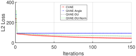
Figure 4: Learning results for classical ligand VAE, quantum VAE with angle embedding, data uploading, and its normalized version.

Two variational autoencoders (VAE), one for the receptor pocket and one for the ligand are constructed for matching pairs of receptor pocket and ligand. The receptor VAE consists of 3D convolutional layers, compressing the original image $R_{0}$ into a 32-element latent representation $R_{c}$ and decompressing back into the original receptor pocket image $R_{d}$. We represent these functions as $E_{R}(R_{0})=R_{c}$, $D_{R}(R_{c})=R_{d}$. Similar ligand VAE architecture is applied except for non-convolutional layers. Two VAEs are connected with a two-way matching network, which converts the latent representation of the receptor pocket into the latent representation of the ligand ($M_{R\rightarrow L}:R_{c}\rightarrow L_{c}$), and vice versa ($M_{L\rightarrow R}:L_{c}\rightarrow R_{c}$). The two directions of the matching network are independent.

For all layers, we use LeakyReLU activation functions and wrap the weights with spectral normalization to prevent exploding/vanishing gradients. Hybrid VAE is created by inserting quantum layers at certain positions in neural networks. Quantum VAE performance are possibly affected by factors, such as quantum embedding techniques, and types of quantum layers. We adopt two currently available quantum embedding techniques i.e., angle embedding and data re-uploading method [18] for measuring different techniques for quantum state preparation. Furthermore, the impact of adding normalization layer immediately after quantum circuit is compared with non-normalized one. Results in Fig. 4 show that QVAE with angle embedding performs poorly, while the classical VAE better in terms of learning speed. Normalized quantum layer helps at the beginning but the effect diminishes as training runs longer. Since no benefit is observed for quantum VAE, we assume the quantum embedding stage restricts the quantum superiority.

IV Conclusion and outlook

We propose drug discovery techniques using QML. We show quantum superiority over classical GAN in terms of architecture complexity, and over classical CNN under the non-parameterized setting, but no superiority is observed over classical VAE. The challenges of QML lie in designing qubit-efficient differentiable quantum embedding technique and developing quantum circuits catered for specific learning tasks.

Acknowledgements: The work is supported in parts by NSF (CNS-1722557, CCF-1718474, OIA-2040667, DGE-1723687 and DGE-1821766) and seed grants from Penn State ICDS and Huck Institute of the Life Sciences. NVD acknowledges support from the National Institutes for Health (1R35 GM134864) and the Passan Foundation. We also thank Mehrdad Mahdavi and Rasit Topaloglu for helpful discussions.

References

- [1] M. Fan et al., “Gpu-accelerated flexible molecular docking,” The Journal of Physical Chemistry B, 2021.
- [2] H. Jiang et al., “Guiding conventional protein-ligand docking software with convolutional neural networks,” Journal of Chemical Information and Modeling, vol. 60, no. 10, pp. 4594–4602, 2020.
- [3] O. Dagliyan et al., “Structural and dynamic determinants of protein-peptide recognition,” Structure, vol. 19, no. 12, pp. 1837–1845, 2011.
- [4] R. A. Friesner et al., “Glide: a new approach for rapid, accurate docking and scoring. 1. method and assessment of docking accuracy,” Journal of medicinal chemistry, 2004.
- [5] F. Ding et al., “Rapid flexible docking using a stochastic rotamer library of ligands,” Journal of chemical information and modeling, 2010.
- [6] J. Wang and N. V. Dokholyan, “Medusadock 2.0: Efficient and accurate protein–ligand docking with constraints,” Journal of chemical information and modeling, vol. 59, no. 6, pp. 2509–2515, 2019.
- [7] O. Trott and A. J. Olson, “Autodock vina: improving the speed and accuracy of docking with a new scoring function, efficient optimization and multithreading,” Journal of computational chemistry, 2010.
- [8] “Rdkit: Open-source cheminformatics; http://www.rdkit.org.”
- [9] J. Li, R. Topaloglu, and S. Ghosh, “Quantum generative models for small molecule drug discovery,” arXiv preprint arXiv:2101.03438, 2021.
- [10] N. De Cao and T. Kipf, “Molgan: An implicit generative model for small molecular graphs,” arXiv preprint arXiv:1805.11973, 2018.
- [11] Z. Wu et al., “Moleculenet,” Chemical science, 2018.
- [12] Y. Du et al., “Expressive power of parametrized quantum circuits,” Physical Review Research, 2020.
- [13] H.-L. Huang et al., “Experimental quantum generative adversarial networks for image generation,” arXiv preprint arXiv:2010.06201, 2020.
- [14] L. Pu et al., “Deepdrug3d,” PLoS computational biology, vol. 15, no. 2, p. e1006718, 2019.
- [15] M. Henderson et al., “Quanvolutional neural networks,” Quantum Machine Intelligence, Springer, 2020.
- [16] V. Bergholm et al., “Pennylane,” arXiv preprint arXiv:1811.04968.
- [17] A. Rahimi, B. Recht et al., “Random features for large-scale kernel machines.” in NIPS, vol. 3, no. 4. Citeseer, 2007, p. 5.
- [18] A. Pérez-Salinas et al., “Data re-uploading for a universal quantum classifier,” arXiv e-prints, p. arXiv:1907.02085, Jul. 2019.