Abstract

Calculations in field theory are usually accomplished by employing some variants of perturbation theory, for instance using loop expansions. These calculations result in asymptotic series in powers of small coupling parameters, which as a rule are divergent for finite values of the parameters. In this paper, a method is described allowing for the extrapolation of such asymptotic series to finite values of the coupling parameters, and even to their infinite limits. The method is based on self-similar approximation theory. This theory approximates well a large class of functions, rational, irrational, and transcendental. A method is presented, resulting in self-similar factor approximants allowing for the extrapolation of functions to arbitrary values of coupling parameters from only the knowledge of expansions in powers of small coupling parameters. The efficiency of the method is illustrated by several problems of quantum field theory.

Keywords: Asymptotic series, self-similar approximation theory, extrapolation problem, Gell-Mann-Low functions, large-variable limit

1 Introduction

The solution of almost all nontrivial problems resorts to the use of some kind of perturbation theory yielding asymptotic series in powers of small parameters. However the physical values of the parameters of interest are usually not small and often are even quite large. Thus we come to the necessity of being able to extrapolate the asymptotic series, that are usually divergent, to the finite values of the parameters of interest. Moreover, sometimes the main interest is in the behaviour of the studied characteristics at asymptotically large parameters tending to infinity. Padé approximants can sometimes extrapolate small-variable series to the finite-variable region. However, as is well known, they cannot describe the large-variable behaviour at the variable tending to infinity, if only a small-variable expansion is available [1]. Let us emphasize that here we keep in mind the case where no large-variable behaviour is known, because of which it is impossible to turn to two-point Padé approximants requiring the knowledge of the large-variable behaviour [1, 2]. Similarly, it is not possible to use other interpolation methods needing the information on the large-variable asymptotic behaviour for the quantity of interest. Our aim here is to consider not interpolation but extrapolation, when only the small-variable expansions are available.

Padé approximants, as is known, provide the best approximation for rational functions, but the reason why they cannot predict the large-variable behavior for irrational functions is rather straightforward. Really a $P_{M/N}(x)$ Padé approximant in the limit of $x\rightarrow\infty$ behaves as $x^{M-N}$, where $M$ and $N$ are integers. Moreover, the difference $M-N$ depends on the used Padé approximant, but not uniquely defines the limiting exponent.

The other method of extrapolation, Borel summation, requires the knowledge of the large-order behaviour of series coefficients, so that the error of the truncated series be bounded by $C^{n}n!|z|^{n}$, where $C$ is a constant [3, 4, 5]. However, this large-order behavior of the expansion coefficients not always is known. There exist several variants of the approach involving Borel summation, including the combination of the Borel transform, conformal mapping, and Padé approximants [3, 4, 5, 6, 7, 8].

Among other methods allowing for the large-variable extrapolation, it is possible to mention the approach based on the introduction of control functions defined by fixed-point conditions optimizing the series convergence [9, 10]. Several variants of this approach have been considered, e.g., [9, 10, 11, 12, 13, 14, 15, 16, 17, 18, 19, 20, 21, 22]. The introduction of control functions requires to rearrange the considered series by either a change of the variable containing trial parameters [4] or by incorporating trial parameters into an initial approximation [9, 10].

The series convergence depends on the choice of an initial approximation. In many cases, one chooses as an initial approximation a Gaussian form corresponding to free particles. More complicated forms for the initial approximation can also be chosen. For example, one can start perturbation theory with a non-Gaussian approximation [23, 24, 25, 26] or one can use for the initial approximation nontrivial Hamiltonians, as in the method of Hamiltonian envelopes [27].

The methods mentioned above are numerical, require rearrangements of perturbation series and rather involved calculations. It would be good to have a simple analytical method that could extrapolate the standard Taylor series derived by the usual perturbation theory in powers of a parameter, say the coupling parameter.

Here we describe such a simple general method allowing for the extrapolation of asymptotic series in powers of a small variable to arbitrary values of this variable, including infinity. As illustration, we accomplish the extrapolation of the series for several functions met in quantum field theory, whose behaviour at large coupling parameters is of interest by its own. The advantages of the suggested approach, as compared to other methods, are as follows.

(i) First of all, the suggested method is analytical allowing for the derivation of explicit forms of the sought functions. This makes it straightforward to analyse the results with respect to different parameters entering the problem, which is not always easy in numerical methods.

(ii) Moreover, numerical methods in some cases are not applicable, while the presented method of extrapolation of asymptotic series can always be applied, provided at least several terms of perturbation theory are available.

(iii) Even if numerical simulations could be invoked, they usually require powerful computational facilities and essential calculational time. On the contrary, the suggested method is very simple and straightforward.

(iv) Numerical methods have their own problems and limitations. Therefore the employment of simpler analytical methods can serve as a guide for numerical calculations.

(v) Finally, the physics of the considered problem becomes much more transparent when possessing an explicit, although approximate, formula allowing for studying its behavior in limiting cases.

It is important to stress that the main aim of the article is to develop a method of extrapolation that would be simple, analytical, and applicable even for those cases where just a few terms of perturbative series are available. This is why we concentrate our attention on these points.

When numerous terms of a series are available, there are several methods allowing for accurate extrapolation. However this is not the point of our interest. If we were interested in getting high accuracy of extrapolation for series with numerous terms, we should resort to some modifications of our method, using additional tricks, such as the introduction of control functions into self-similar approximants [21], the combination of self-similar approximations with Pade approximants or with Borel transforms, etc. Thus it has been demonstrated [28, 29] that the combination of self-similar and Padé approximants converges much faster and provides essentially higher accuracy then the best Padé approximants of the same order. However all that is a quite different problem requiring separate investigations and publications, some of which we cite. We stress it again that the main aim of the present paper is to suggest a simple analytical method providing reliable approximations when other methods are not applicable.

2 Self-similar approximation theory

The suggested method is based on self-similar approximation theory advanced in Refs. [30, 31, 32, 33, 34]. In Ref. [35], this theory is used for developing a convenient approach to the problems of interpolation in high-energy physics, when weak-coupling as well as strong-coupling expansions are known. Here we extend the applicability of the approach for the essentially more complicated problem of extrapolation in quantum field theory, when only the weak-coupling asymptotic series are available, but the behavior at the strong-coupling limit is not known, and even more, finding this behavior is the point of main interest.

First we briefly recall the main ideas of self-similar approximation theory in order that the reader could understand its justifications and would get the feeling why it can successfully work. This approach is based on mathematical techniques of renormalization group theory, dynamical theory, and optimal control theory [36, 37, 38]. Note that these theories are closely interrelated since the renormalization group theory, actually, is a particular case of dynamical theory.

The pivotal idea is to reformulate perturbation theory to the language of dynamical theory or renormalization-group theory. For this purpose, we treat the approximation-order index as discrete time and the passage from one approximation to another as the motion in the space of approximations. Suppose, we can find the sought function only as a sequence of approximations at a small variable, $f(x)\simeq f_{k}(x)$ for $x\rightarrow 0$, where $k=0,1,2,\ldots$ is the approximation order. For concreteness, we consider here real-valued functions of real variables. The extension to complex-valued functions can be straightforwardly done by considering several functions corresponding to real and imaginary parts of the sought function.

The sequence of the bare approximants $f_{k}(x)$ is usually divergent. Therefore the first thing that is necessary to do is to reorganize this sequence by introducing control functions $u_{k}=u_{k}(x)$ governing the sequence convergence. Control functions can be incorporated in several ways, through initial conditions, calculational algorithm, or by a sequence transformation. Thus, instead of the bare approximants $f_{k}(x)$, we pass to a transformed sequence of the approximants

$$F_{k}(x,u_{k})=\hat{T}[u]f_{k}(x)\;.$$

For short, we write here one control function $u_{k}$, although there can be several of them, so that $u_{k}$ can be understood as a set of the necessary control functions. We assume that the used transformation is invertible, in the sense that

$$f_{k}(x)=\hat{T}^{-1}[u]F_{k}(x,u_{k})\;.$$

The sequence $\{F_{k}(x,u_{k})\}$ is convergent if and only if it satisfies the Cauchy criterion, when for each $\varepsilon>0$ there exists a number $k_{c}$ such that

$$|F_{k+p}(x,u_{k+p})-F_{k}(x,u_{k})|<\varepsilon$$

for all $k>k_{c}$ and $p>0$. In the language of optimal control theory, this implies that control functions can be defined as the minimizers of the convergence cost functional [38]

$$C[u]=\sum_{k}|F_{k+1}(x,u_{k+1})-F_{k}(x,u_{k})|\;.$$ (1)

In order to formulate the passage between different $F_{k}$ as the evolution of a dynamical system, it is necessary to define an endomorphism in the space of approximants

$${\cal A}=\{F_{k}(x):\;k=0,1,2,\ldots;\;x\in\mathbb{R}\}\;.$$

For this purpose, we introduce the expansion function $x=x_{k}(f)$ by the reonomic constraint

$$F_{0}(x,u_{k}(x))=f\;.$$

The endomorphism in the approximation space is defined as

$$y_{k}(f)\equiv F_{k}(x_{k}(f),u_{k}(x_{k}(f)))\;,$$

with the inverse relation

$$F_{k}(x,u_{k}(x))=y_{k}(F_{0}(x,u_{k}(x)))\;.$$

By this construction, the approximation sequence $\{F_{k}\}$ is bijective with the sequence of the endomorphisms $\{y_{k}\}$. Therefore, if the sequence $\{F_{k}\}$ converges to a limit $F^{*}$, then the sequence of the endomorphisms $\{y_{k}\}$ converges to a limit $y^{*}$. The limit $y^{*}$ plays the role of a fixed point for the endomorphism sequence $\{y_{k}\}$, where $y_{k}(y^{*}(f))=y^{*}(f)$. In the vicinity of a fixed point, the endomorphism enjoys the property of self-similarity

$$y_{k+p}(f)=y_{k}(y_{p}(f))\;,$$ (2)

with the initial condition $y_{0}(f)=f$. This is, actually, just the semi-group property $y_{k+p}=y_{k}\cdot y_{p}$, with the unity element $y_{0}=1$. The sequence of endomorphisms, with the above semi-group property, is called cascade (or semi-cascade),

$$\{y_{k}(f):\;\mathbb{Z}_{+}\times\mathbb{R}~{}\rightarrow~{}\mathbb{R}\}\;,$$

where the role of time is played by the approximation order $k$.

A cascade , which is a dynamical system in discrete time, can be embedded [39] into a flow that is a dynamical system in continuous time,

$$\{y_{k}(f):\;\mathbb{Z}_{+}\times\mathbb{R}\rightarrow\mathbb{R}\}\subset\{y(t,f):~{}\mathbb{R}_{+}\times\mathbb{R}~{}\rightarrow~{}\mathbb{R}\}\,.$$

The embedding implies that the flow enjoys the same group property

$$y(t+t^{\prime},f)=y(t,y(t^{\prime},f))$$

and the flow trajectory passes through all points of the cascade trajectory,

$$y(t,f)=y_{k}(f)\qquad(t=k)\;,$$

with the same initial condition $y(0,f)=f$.

The above group property can be rewritten as the Lie differential equation

$$\frac{\partial}{\partial t}\;y(t,f)=v(y(t,f))\;,$$ (3)

with the velocity

$$v(y)\equiv\lim_{\tau\rightarrow 0}\;\frac{\partial}{\partial\tau}\;y(\tau,y)\;.$$

Integrating the differential evolution equation (3) yields the evolution integral

$$\int_{y_{k}}^{y_{k}^{*}}\frac{dy}{v(y)}=t_{k}\;,$$ (4)

in which the integration is from a point $y_{k}(f)$ to an approximate fixed point $y_{k}^{*}(f)$, with $t_{k}$ being the effective time needed for reaching the latter point. Here $y_{k}^{*}(f)$ is an approximate fixed point, since in practice we always have to limit the consideration by a finite number of steps. Taking in the evolution integral the cascade velocity represented in the form of the Euler discretization

$$v_{k}(f)=y_{k+1}(f)-y_{k}(f)\;,$$

we come to the integral

$$\int_{F_{k}}^{F_{k}^{*}}\frac{df}{v_{k}(f)}=t_{k}\;,$$ (5)

in which

$$F_{k}^{*}(x)=y_{k}^{*}(F_{0}(x,u_{k}(x))$$

is the effective limit of the sequence $\{F_{k}\}$ corresponding to the approximate fixed point $y^{*}_{k}$. Applying the inverse transformation, we obtain the self-similar approximant

$$f_{k}^{*}(x)=\hat{T}^{-1}[u]F_{k}^{*}(x)\;.$$

These are the principal steps in deriving self-similar approximants. The practical realization depends on the form of the bare approximants $f_{k}(x)$, the concrete form of the transformation $\hat{T}$ introducing control functions, and on the method of defining the latter. When the asymptotic behaviour of the sought quantity is known for small as well as for large coupling parameters, it is convenient to accomplish the interpolation with the use of self-similar root approximants, as is demonstrated in Ref. [35]. But for the problem of extrapolation we need to employ another type of approximants.

Usually, the asymptotic behaviour at small coupling parameters $x\rightarrow 0$, is of the form

$$f_{k}(x)=f_{0}(x)\left(1+\sum_{n=1}^{k}a_{n}x^{n}\right)\;,$$ (6)

where $f_{0}(x)$ is a given function. The above sum is usually divergent for finite values of $x$, hence makes no sense for finite $x$. Moreover, often it is necessary to find the behaviour of the sought function $f(x)$ at asymptotically large $x\rightarrow\infty$.

By the fundamental theorem of algebra [40], a polynomial of any degree of one real variable over the field of real numbers can be split in a unique way into a product of irreducible first-degree polynomials over the field of complex numbers. This implies that the finite series (6) can be represented as the product

$$f_{k}(x)=f_{0}(x)\prod_{j}\left(1+b_{j}x\right)\;,$$ (7)

with $b_{j}$ expressed through $a_{n}$.

Control functions can be explicitly incorporated by employing fractal transforms [38, 41], which can be written in the form

$$\hat{T}[s,u]f_{k}(x)=x^{s_{k}}f_{k}(x)+u_{k}\;.$$ (8)

Then, following the scheme described above, we obtain the self-similar factor approximants

$$f_{k}^{*}(x)=f_{0}(x)\prod_{j=1}^{N_{k}}\left(1+A_{j}x\right)^{n_{j}}\;,$$ (9)

with $A_{j}$ and $n_{j}$ playing the role of control parameters [42, 43, 44].

The number of factors $N_{k}$ equals $k/2$ for even $k$ and $(k+1)/2$ for odd $k$. A factor approximant (9) represents the sought function, therefore their asymptotic expansions should coincide. Then the parameters $A_{j}$ and $n_{j}$ are to be chosen so that the asymptotic expansion of approximant (9) of order $k$ be equal to the asymptotic form (6), that is, $f_{k}^{*}(x)\simeq f_{k}(x)$ for $x\rightarrow 0$. This condition yields the equations

$$\sum_{j=1}^{N_{k}}n_{j}A_{j}^{n}=D_{n}\qquad(n=1,2,\ldots,k)\;,$$ (10)

where

$$D_{n}\equiv\frac{(-1)^{n-1}}{(n-1)!}\;\lim_{x\rightarrow 0}\;\frac{d^{n}}{dx^{n}}\;\ln\left(1+\sum_{m=1}^{n}a_{m}x^{m}\right)\;.$$

When $k$ is even, hence $N_{k}=k/2$, we have $k$ equations for $k$ unknown parameters $A_{j}$ and $n_{j}$, uniquely defining these parameters [44]. However if $k$ is odd, and $N_{k}=(k+1)/2$, we have $k$ equations for $k+1$ parameters. Then, to make the system of equations complete, it is necessary to add one more condition. For instance, resorting to scaling arguments [44], it is possible to set one of $A_{j}$ to one, say fixing $A_{1}=1$. This method gives for odd approximants the results close to the nearest even-order approximants. However below we prefer to deal with uniquely defined even orders. Sometimes it may happen that the solutions for the parameters $A_{j}$ and $n_{j}$ are complex-valued. But this does not lead to any problem, since such complex solutions for the parameters appear in complex conjugate pairs, so that the whole expression remains real valued.

When we are interested in predicting the large-variable behaviour of a function $f(x)$, we study the self-similar factor approximant (9) at $x\rightarrow\infty$. If the function $f_{0}$ behaves as $f_{0}(x)\simeq Ax^{\alpha}$ for $x\rightarrow\infty$, then the self-similar factor approximant (9) for large $x$ is

$$f_{x}^{*}(x)\simeq B_{k}x^{\gamma_{k}}\qquad(x\rightarrow\infty)\;,$$ (11)

with the amplitude and the exponent

$$B_{k}=A\prod_{j=1}^{N_{k}}A_{j}^{n_{j}}\;,\qquad\gamma_{k}=\alpha+\sum_{j=1}^{N_{k}}n_{j}\;.$$ (12)

In those cases, where the large-variable asymptotic behaviour of the sought function is known, say being $f(x)\simeq Bx^{\gamma}$ for $x\rightarrow\infty$, it is straightforward to determine the accuracy of the prediction by calculating the percentage errors $\varepsilon(B_{k})\equiv((B_{k}-B)/B)\times 100\%$ and $\varepsilon(\gamma_{k})\equiv((\gamma_{k}-\gamma)/\gamma)\times 100\%$. When the exact large-variable asymptotic behaviour is not available, one usually presents the difference between the subsequent approximations for the quantity of interest. This difference characterizes the variation bar or dispersion of the obtained results, which is related to the stability of the calculational procedure [45]. If the subsequent results strongly differ from each other, this induces suspicion of the procedure stability.

Often, the most important hard case is the prediction of the exponent in the strong-coupling limit, since the value of the exponent essentially defines the physics of the problem. This hard case is the main study in the present article.

It is important to stress that the derivation of self-similar factor approximants is based on the Cauchy criterion of convergence, so that these approximants are expected to converge by construction. Moreover the numerical convergence of self-similar factor approximants has been confirmed by a number of problems enjoying many terms in their asymptotic expansions, when a long sequence of the factor approximants could be considered [38, 42, 43, 44, 46]. It has been shown that for finite values of the considered variable the accuracy of self-similar approximants is comparable with that of heavy numerical calculations. In the present paper we concentrate on the most difficult and interesting challenge of finding strong-coupling limits of functions, especially their exponents, from the knowledge of only a few terms in their asymptotic weak-coupling expansions. This type of problems is difficult even for numerical methods. The approach is illustrated by several problems of quantum field theory.

3 Convergence of self-similar factor approximants

When a number of terms in a weak-coupling expansion are available and the asymptotic behavior in the strong-coupling limit is known, it is possible to study numerical convergence of the approximants. Below we illustrate this by several examples.

3.1 Zero-dimensional $\varphi^{4}$ theory

Let us start with the simple example of the so-called zero-dimensional $\varphi^{4}$ theory characterized by the generating functional (partition function)

$$Z(g)=\frac{1}{\sqrt{\pi}}\int_{-\infty}^{\infty}e^{-\varphi^{2}-g\varphi^{4}}\;d\varphi\;,$$ (13)

with the coupling parameter $g\geq 0$. The weak-coupling asymptotic expansion reads as

$$Z_{k}(g)=\sum_{n=0}^{k}a_{n}g^{n}\qquad(g\rightarrow 0)\;,$$ (14)

where the coefficients are

$$a_{n}=\frac{(-1)^{n}}{\sqrt{\pi}\;n!}\;\Gamma\left(2n+\frac{1}{2}\right)\;.$$

Using only this weak-coupling expansion, we construct the self-similar factor approximants and study their strong-coupling limit, which gives

$$Z_{k}^{*}(g)\simeq B_{k}g^{\gamma_{k}}\qquad(g\rightarrow\infty)\;.$$ (15)

The accuracy of the obtained strong-coupling exponents can be found by comparing the above limit with the known strong-coupling behavior

$$Z(g)\simeq 1.022765\;g^{-1/4}\qquad(g\rightarrow\infty)\;.$$ (16)

The results, shown in Table 1, demonstrate monotonic convergence to the exact limiting value $-0.25$. In the $16$-th order, we have

$$Z_{16}^{*}(g)\simeq 0.828\;g^{-0.187}\qquad(g\rightarrow\infty)\;.$$ (17)

Table 1: Strong-coupling exponents and their percentage errors for the generating functional of zero-dimensional $\varphi^{4}$ theory.

$k$	2	4	6	8	10	12	14	16
$\gamma_{k}$	$-0.09$	$-0.13$	$-0.15$	$-0.16$	$-0.17$	$-0.18$	$-0.18$	$-0.19$
$\varepsilon(\gamma_{k})\%$	$-$63	$-$48	$-$41	$-$36	$-$32	$-$29	$-$27	$-$25

3.2 One-dimensional anharmonic oscillator

The one-dimensional anharmonic oscillator with the Hamiltonian

$$H=-\;\frac{1}{2}\;\frac{d^{2}}{dx^{2}}+\frac{1}{2}\;x^{2}+gx^{4}\;,$$ (18)

where $g\geq 0$ and $-\infty<x<\infty$, imitates the one-dimensional $\varphi^{4}$ theory. The weak-coupling expansion of the ground-state energy is

$$E_{k}(g)\simeq\frac{1}{2}+\sum_{n=0}^{k}a_{n}g^{n}\qquad(g\rightarrow 0)\;,$$ (19)

with the coefficients that can be found in Refs. [47, 48].

Constructing the factor approximants and looking for their strong-coupling limit

$$E_{k}^{*}(g)\simeq B_{k}g^{\gamma_{k}}\qquad(g\rightarrow\infty)$$ (20)

yields the results for the exponents shown in Table 2. The accuracy is found by the comparison with the known strong-coupling asymptotic behavior

$$E(g)\simeq 0.667986\;g^{1/3}\qquad(g\rightarrow\infty)\;.$$ (21)

In the $16$-th order, we get

$$E_{16}^{*}(g)\simeq 0.736\;g^{0.298}\qquad(g\rightarrow\infty)\;.$$ (22)

Table 2 demonstrates monotonic numerical convergence.

Table 2: Strong-coupling exponents and their percentage errors for the ground-state energy of one-dimensional ahharmonic oscillator.

$k$	2	4	6	8	10	12	14	16
$\gamma_{k}$	0.18	0.23	0.26	0.27	0.28	0.29	0.29	0.30
$\varepsilon(\gamma_{k})\%$	$-$47	$-$31	$-$23	$-$18	$-$16	$-$13	$-$12	$-$11

3.3 Massive Schwinger model in lattice theory

One of the simplest nontrivial gauge-theory models is the Schwinger model [49]. This is a lattice model of quantum electrodynamics in $1+1$ space-time dimensions. The model exhibits several phenomena typical of quantum chromodynamics, such as confinement, chiral symmetry breaking with an axial anomaly, and a topological vacuum [50, 51, 52, 53, 54]. The spectrum of excited states for a finite lattice, calculated by means of perturbation theory, is expressed through the series

$$f_{k}(z)\simeq 1+\sum_{k=1}^{k}a_{n}z^{n}\qquad(z\rightarrow 0)$$ (23)

in powers of the variable $z\equiv 1/(ga)^{4}$, where $g$ is the coupling parameter and $a$ is the lattice spacing [55]. The coefficients for the vector boson are

$$a_{1}=2\;,\qquad a_{2}=-10\;,\qquad a_{3}=78.66667\;,\qquad a_{4}=-7.362222\times 10^{2}\;,$$

$$a_{5}=7.572929\times 10^{3}\;,\qquad a_{6}=-8.273669\times 10^{4}\;,\qquad a_{7}=9.428034\times 10^{5}\;,$$

$$a_{8}=-1.108358\times 10^{7}\;,\qquad a_{9}=1.334636\times 10^{8}\;,\qquad a_{10}=-1.637996\times 10^{9}\;.$$

Constructing factor approximants and considering their large-$z$ limit, we have

$$f_{k}^{*}(z)\simeq B_{k}z^{\gamma_{k}}\qquad(z\rightarrow\infty)\;,$$ (24)

with the results for the large-$z$ exponent listed in Table 3. This is to be compared with the known limiting behavior

$$f(z)\simeq 1.1284z^{1/4}\qquad(z\rightarrow\infty)\;.$$ (25)

For example, in the $10$-th order

$$f_{10}^{*}(z)\simeq 1.519\;z^{0.2}\qquad(z\rightarrow\infty)\;.$$ (26)

Table 3: Large-$z$ exponents and their percentage errors for the function $f(z)$ of the finite-lattice Schwinger model.

$k$	2	4	6	8	10
$\gamma_{k}$	0.167	0.185	0.193	0.198	0.200
$\varepsilon(\gamma_{k})\%$	$-$33	$-$26	$-$23	$-$21	$-$20

3.4 Ground-state energy of Schwinger model

The ground-state energy of the Schwinger model with a vector boson, in the continuum limit, can be found [51, 52, 53, 54] as an expansion in powers of the dimensionless variable $x=m/g$, where $m$ is the electron mass and $g$ is the coupling parameter,

$$\frac{E(x)}{g}\simeq 0.5642-0.219x+0.1907x^{2}\qquad(x\rightarrow 0)\;.$$ (27)

This short series allows us to construct only the second-order factor approximant

$$\frac{E_{2}^{*}(x)}{g}=\frac{0.5642}{(1+1.35339x)^{0.286805}}\;.$$ (28)

In the large-$x$ limit this gives

$$\frac{E_{2}^{*}(x)}{g}\simeq 0.5173x^{-0.287}\qquad(x\rightarrow\infty)\;.$$ (29)

Comparing the large-$x$ exponent, with the known asymptotic behavior [54, 55, 56, 57]

$$\frac{E(x)}{g}\simeq 0.6417x^{-1/3}\qquad(x\rightarrow\infty)\;,$$ (30)

we find that the percentage error of the predicted exponent is $\varepsilon(\gamma_{2})=-14\%$.

3.5 Summary for considered examples

The above examples show that the knowledge of only a small-variable asymptotic expansion makes it possible to extrapolate the small-variable expansion to finite-values of the variable and even to predict the behavior of the corresponding function at asymptotically large values of the variable. When a number of terms in the small-variable series are known, the sequence of the related self-similar approximants is shown to converge. The self-similar extrapolation allows for sufficiently accurate evaluation of the large-variable exponent even when just a few terms of the small-variable expansion are available.

The reason why a small-variable expansion can be extrapolated to the finite and even infinite values of the variable lays in the following. The coefficients of the expansion contain hidden information on the whole function which they are derived from. Separate coefficients do not allow for noticing this hidden information. However this information can be extracted by analyzing the relations between the coefficients. Self-similar approximation theory provides an instrument revealing the relations between the expansion coefficients and thus allowing for the reconstruction of the whole sought function.

4 Exact reconstruction of Gell-Mann-Low functions

Gell-Mann-Low functions in quantum field theory are usually calculated by means of loop expansions yielding series in powers of asymptotically small coupling parameters. However, the behaviour of these functions at strong coupling is of special interest. Below we consider the extrapolation of these functions to the arbitrary values of coupling parameters, including the limit to $\infty$, by employing self-similar factor approximants. A special attention will be paid to the study of the strong-coupling limit. In the present section, we demonstrate that in some cases, having just a few perturbative terms, self-similar approximants can reconstruct the sought Gell-Mann-Low function exactly.

For this purpose, let us turn to the $N=1$ supersymmetric pure Yang-Mills theory whose exact beta function is known [58, 59, 60, 61, 62, 63]:

$$\beta(g)=-\;\frac{3g^{3}N_{c}}{16\pi^{2}(1-g^{2}N_{c}/8\pi^{2})}\;.$$ (31)

If one resorts to perturbation theory with respect to the coupling $g$, one gets

$$\beta_{k}(g)=-\;\frac{3g^{3}N_{c}}{16\pi^{2}}\sum_{n=0}^{k}b_{n}g^{2n}\;,$$ (32)

with the coefficients

$$b_{n}=\left(\frac{N_{c}}{8\pi^{2}}\right)^{n}\;.$$

For the second-order factor approximant, we have

$$\beta_{2}^{*}(g)=-\;\frac{3g^{3}N_{c}}{16\pi^{2}}\;\left(1+A_{1}g^{2}\right)^{n_{1}}\;.$$ (33)

Expanding Eq. (33) and comparing the expansion with series (32) yields

$$n_{1}=-1\;,\qquad A_{1}=-\;\frac{N_{c}}{8\pi^{2}}\;.$$

Thus the second-order factor approximant results in the exact expression (31). It is easy to check that all approximants of orders $k\geq 2$ give the exact beta function (31).

5 Gell-Mann-Low function in $\varphi^{4}$ field theory

Let us consider the $O(N)$ symmetric $\varphi^{4}$ field theory. The Gell-Mann-Low function is defined as

$$\beta(g)=\mu\;\frac{\partial g}{\partial\mu}\;,$$ (34)

where $g=\lambda/(4\pi)^{2}$ is the coupling parameter and $\mu$ is renormalization scale. This function has been found [64], within minimal subtraction scheme, in the six-loop approximation:

$$\beta(g)\simeq g^{2}\sum_{n=0}^{k}b_{n}g^{n}\qquad(g\rightarrow 0)\;,$$ (35)

with the coefficients

$$b_{0}=\frac{N+8}{3}\;,\qquad b_{1}=-\;\frac{3N+14}{3}\;,$$

$$b_{2}=\frac{1}{216}\left[96(5N+22)\zeta(3)+33N^{2}+922N+2960\right]\;,$$

$$b_{3}=-\;\frac{1}{3888}\left[1920\left(2N^{2}+55N+186\right)\zeta(5)-288(N+8)(5N+22)\zeta(4)+\right.$$

$$+\left.96\left(63N^{2}+764N+2332\right)\zeta(3)-\left(5N^{3}-6320N^{2}-80456N-196648\right)\right]\;,$$

$$b_{4}=\frac{1}{62208}\left[112896\left(14N^{2}+189N+526\right)\zeta(7)-768\left(6N^{3}+59N^{2}-446N-3264\right)\zeta^{2}(3)-\right.$$

$$-9600(N+8)\left(2N^{2}+55N+186\right)\zeta(6)+256\left(305N^{3}+7466N^{2}+66986N+165084\right)\zeta(5)-$$

$$-288\left(63N^{3}+1388N^{2}+9532N+21120\right)\zeta(4)-$$

$$-16\left(9N^{4}-1248N^{3}-67640N^{2}-552280N-1314336\right)\zeta(3)+$$

$$+\left.13N^{4}+12578N^{3}+808496N^{2}+6646336N+13177344\right]\;,$$

$$b_{5}=-\;\frac{1}{41990400}\left[204800\left(1819N^{3}+97823N^{2}+901051N+2150774\right)\zeta(9)+\right.$$

$$+14745600\left(N^{3}+65N^{2}+619N+1502\right)\zeta^{3}(3)+$$

$$+995328\left(42N^{3}+2623N^{2}+25074N+59984\right)\zeta(3,5)-$$

$$-20736\left(28882N^{3}+820483N^{2}+6403754N+14174864\right)\zeta(8)-$$

$$-5529600\left(8N^{3}-635N^{2}-9150N-25944\right)\zeta(3)\zeta(5)+$$

$$+11520\left(440N^{4}+126695N^{3}+2181660N^{2}+14313152N+29762136\right)\zeta(7)+$$

$$+207360(N+8)\left(6N^{3}+59N^{2}-446N-3264\right)\zeta(3)\zeta(4)-$$

$$-23040\left(188N^{4}+132N^{3}-93363N^{2}-862604N-2207484\right)\zeta^{2}(3)-$$

$$-28800\left(595N^{4}+20286N^{3}+277914N^{2}+1580792N+2998152\right)\zeta(6)+$$

$$+5760\left(4698N^{4}+131827N^{3}+2250906N^{2}+14657556N+29409080\right)\zeta(5)+$$

$$+2160\left(9N^{5}-1176N^{4}-88964N^{3}-1283840N^{2}-6794096N-12473568\right)\zeta(4)-$$

$$-720\left(33N^{5}+2970N^{4}-477740N^{3}-10084168N^{2}-61017200N-117867424\right)\zeta(3)-$$

$$-\left.45\left(29N^{5}+22644N^{4}-3225892N^{3}-88418816N^{2}-536820560N-897712992\right)\right]\;.$$

Here $\zeta(3,5)$ denotes the double zeta function

$$\zeta(3,5)=\sum_{1\leq n<m}\frac{1}{n^{3}m^{5}}=0.037707673\;.$$

The numerical values of the coefficients for the number of components from $N=0$ to $N=4$ are given in Table 4.

Table 4: Coefficients of weak-coupling expansion for the Gell-Man-Low function of the $N$-component $\varphi^{4}$ field theory, in the six-loop approximation.

$N$	0	1	2	3	4
$b_{0}$	2.66667	3.0	3.33333	3.66667	4.0
$b_{1}$	$-$4.66667	$-$5.66667	$-$6.66667	$-$7.66667	$-$8.66667
$b_{2}$	25.4571	32.5497	39.9478	47.6514	55.6606
$b_{3}$	$-$200.926	$-$271.606	$-$350.515	$-$437.646	$-$532.991
$b_{4}$	2003.98	2848.57	3844.51	4998.62	6317.66
$b_{5}$	$-$23314.7	$-$34776.1	$-$48999.1	$-$66242.7	$-$86768.4

In the case of $N=1$, the Gell-Mann-Low function is known in the seven-loop approximation [65] having the coefficients

$$b_{0}=3\;,\qquad b_{1}=-5.66667\;,\qquad b_{2}=32.5497\;,\qquad b_{3}=-271.606\;,$$

$$b_{4}=2848.57\;,\qquad b_{5}=-34776.1\;,\qquad b_{6}=474651\;.$$

We construct self-similar factor approximants for different $N$. Thus for $N=0$, we have

$$\beta_{2}^{*}(g)=\frac{2.66667g^{2}}{(1+9.16021g)^{0.191044}}\qquad(N=0)\;,$$

$$\beta_{4}^{*}(g)=\frac{2.66667g^{2}}{(1+6.06377g)^{0.194059}(1+15.5161g)^{0.0369468}}\;,$$ (36)

which yields the strong-coupling limit

$$\beta_{2}^{*}(g)\simeq 1.747g^{1.809}\;,\qquad\beta_{4}^{*}(g)\simeq 1.699g^{1.769}\qquad(N=0,~{}g\rightarrow\infty)\;.$$ (37)

For $N=2$, we find

$$\beta_{2}^{*}(g)=\frac{3.33333g^{2}}{(1+9.98433g)^{0.200314}}\qquad(N=2)\;,$$

$$\beta_{4}^{*}(g)=\frac{3.33333g^{2}}{(1+5.79973g)^{0.206354}(1+16.2195g)^{0.0495207}}\;,$$ (38)

with the strong-coupling limit

$$\beta_{2}^{*}(g)\simeq 2.102g^{1.7997}\;,\qquad\beta_{4}^{*}(g)\simeq 2.020g^{1.7441}\qquad(N=2,~{}g\rightarrow\infty)\;.$$ (39)

For $N=3$, we obtain

$$\beta_{2}^{*}(g)=\frac{3.66667g^{2}}{(1+10.3399g)^{0.202218}}\qquad(N=3)\;,$$

$$\beta_{4}^{*}(g)=\frac{3.66667g^{2}}{(1+5.53502g)^{0.212617}(1+16.526g)^{0.055311}}\;,$$ (40)

giving the limit

$$\beta_{2}^{*}(g)\simeq 2.286g^{1.798}\;,\qquad\beta_{4}^{*}(g)\simeq 2.182g^{1.732}\qquad(N=3,~{}g\rightarrow\infty)\;.$$ (41)

And for the case of $N=4$, we get

$$\beta_{2}^{*}(g)=\frac{4g^{2}}{(1+10.6781g)^{0.202908}}\qquad(N=4)\;,$$

$$\beta_{4}^{*}(g)=\frac{4g^{2}}{(1+5.2767g)^{0.219241}(1+16.8661g)^{0.0598713}}\;,$$ (42)

with the strong-coupling limit

$$\beta_{2}^{*}(g)\simeq 2.474g^{1.797}\;,\qquad\beta_{4}^{*}(g)\simeq 2.345g^{1.721}\qquad(N=4,~{}g\rightarrow\infty)\;.$$ (43)

For $N=1$, we use the seven-loop expansion obtaining the functions

$$\beta_{2}^{*}(g)=\frac{3g^{2}}{(1+9.59923g)^{0.196775}}\qquad(N=1)\;,$$

$$\beta_{4}^{*}(g)=\frac{3g^{2}}{(1+6.01378g)^{0.200415}(1+15.9204g)^{0.0429409}}\;,$$

$$\beta_{6}^{*}(g)=\frac{3g^{2}}{(1+5.35692g)^{0.186798}(1+13.7203g)^{0.0596501}(1+22.0958g)^{0.0031595}}\;,$$ (44)

whose strong-coupling behavior is

$$\beta_{2}^{*}(g)\simeq 1.922g^{1.803}\;,\qquad\beta_{4}^{*}(g)\simeq 1.859g^{1.757}\;,$$

$$\beta_{6}^{*}(g)\simeq 1.857g^{1.750}\qquad(N=1,~{}g\rightarrow\infty)\;.$$ (45)

Summarizing, we present in Table 5 the averaged results

$$B=\frac{1}{k}\sum_{n=1}^{k}B_{2n}\;,\qquad\gamma=\frac{1}{k}\sum_{n=1}^{k}\gamma_{2n}$$ (46)

for the amplitudes and exponents characterizing the strong-coupling limit

$$\beta(\gamma)\simeq Bg^{\gamma}\qquad(g\rightarrow\infty)\;,$$ (47)

together with the dispersion between the subsequent approximants.

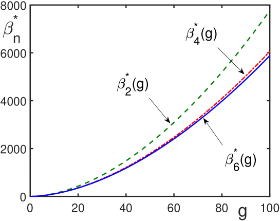
Figure 1: Gell-Mann-Low function of $\varphi^{4}$ $O(1)$ symmetric field theory as a function of the coupling parameter $g$. The convergence of the approximants of second, fourth, and sixth order is evident.

The overall behaviour of the Gell-Mann-Low function of $\varphi^{4}$ field theory for $N=1$ is shown in Fig. 1, where the convergence of the approximants is evident. The behaviour of the Gell-Mann-Low functions for other $N$ is similar, only slightly differing from that for $N=1$.

In literature, it is possible to find the estimates for the strong-coupling exponent $\gamma$ in the case of $N=1$. Thus Borel summation with conformal mapping gives $\gamma=2$ [66] or $\gamma=1.9$ [67]. A variational estimate [68] yields $\gamma=1.5$. Our result of $\gamma=1.77$ for $N=1$ is between those given by the Borel summation and variational calculations.

Table 5: Strong-coupling amplitudes and exponents for the $N$-component $\varphi^{4}$ field theory, predicted by self-similar factor approximants.

$N$	B	$\gamma$
0	$1.723\pm 0.02$	$1.789\pm 0.02$
1	$1.879\pm 0.03$	$1.770\pm 0.03$
2	$2.061\pm 0.04$	$1.772\pm 0.03$
3	$2.235\pm 0.05$	$1.765\pm 0.03$
4	$2.410\pm 0.06$	$1.759\pm 0.04$

6 Gell-Mann-Low function in quantum electrodynamics

In quantum electrodynamics, the Gell-Mann-Low function in the renormalized minimal subtraction scheme $(\overline{\rm MS})$ reads as

$$\beta(\alpha)=\mu^{2}\;\frac{\partial}{\partial\mu^{2}}\left(\frac{\alpha}{\pi}\right)\;,$$ (48)

where $\alpha$ is the renormalized $(\overline{\rm MS})$ scheme coupling parameter and $\mu$ is the $(\overline{\rm MS})$ scale parameter. The weak-coupling expansion in five-loop approximation, taking into account the electron, but neglecting the contributions of leptons with higher masses, that is, muons and tau-leptons, has the form [69]

$$\beta(\alpha)\simeq\left(\frac{\alpha}{\pi}\right)^{2}\sum_{n=0}^{k}b_{n}\left(\frac{\alpha}{\pi}\right)^{n}\;,$$ (49)

with the coefficients

$$b_{0}=\frac{1}{3}=0.333333\;,\qquad b_{1}=\frac{1}{4}\;,\qquad b_{2}=-\;\frac{31}{288}=-0.107639\;,$$

$$b_{3}=-\;\frac{2785}{31104}\;-\;\frac{13}{36}\;\zeta(3)=-0.523614\;,$$

$$b_{4}=-\;\frac{195067}{497664}\;-\;\frac{25}{96}\;\zeta(3)\;-\;\frac{13}{96}\;\zeta(4)\;+\;\frac{215}{96}\;\zeta(5)=1.47072\;.$$

From here, we find the factor approximants

$$\beta_{2}^{*}(\alpha)=\frac{1}{3}\left(\frac{\alpha}{\pi}\right)^{2}\left(1+1.61111\;\frac{\alpha}{\pi}\right)^{0.465517}\;,$$

$$\beta_{4}^{*}(\alpha)=\frac{1}{3}\left(\frac{\alpha}{\pi}\right)^{2}\left(1+A_{1}\;\frac{\alpha}{\pi}\right)^{n_{1}}\left(1+A_{2}\;\frac{\alpha}{\pi}\right)^{n_{2}}\;$$ (50)

where

$$A_{1}=1.394295+2.70199797\;i=A_{2}^{*}\;,\qquad n_{1}=0.047762-0.11413974\;i=n_{2}^{*}\;.$$

Therefore in the strong-coupling limit, we have

$$\beta_{2}^{*}(\alpha)\simeq 0.4162\left(\frac{\alpha}{\pi}\right)^{2.4655}\;,$$

$$\beta_{4}^{*}(\alpha)\simeq 0.4759\left(\frac{\alpha}{\pi}\right)^{2.0955}\qquad\left(\frac{\alpha}{\pi}\rightarrow\infty\right)\;.$$ (51)

Defining average quantities, we see that the strong-coupling behaviour of the Gell-Mann-Low function

$$\beta(\alpha)\simeq B\left(\frac{\alpha}{\pi}\right)^{\gamma}\qquad\left(\frac{\alpha}{\pi}\rightarrow\infty\right)$$ (52)

can be characterized by the amplitude and exponent

$$B=0.446\pm 0.03\;,\qquad\gamma=2.281\pm 0.19\;.$$ (53)

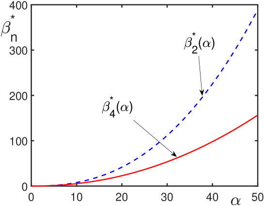
Figure 2: Gell-Mann-Low function of quantum electrodynamics as a function of the coupling parameter $\alpha$.

The dependence of the Gell-Mann-Low function for quantum electrodynamics is presented in Fig. 2. Its overall behaviour only slightly depends on the chosen scheme. Thus, accepting the coefficients of the weak-coupling expansion found in the on-shell scheme or in the momentum subtraction scheme [69] results in $B=0.433,\;\gamma=2.189$ in the on-shell scheme and $B=0.493,\;\gamma=2.309$ in the momentum subtraction scheme.

The running coupling defined by equation (48), with the beta function represented by a factor approximant, increases from zero to infinity. As the boundary condition, we can take the value $\alpha(m_{Z})=0.007815$ at the $Z$-boson mass $m_{Z}=91.1876$ GeV. Then the logarithmic divergence occurs at $\mu_{0}=8.584\times 10^{260}$ GeV, where

$$\alpha\simeq\frac{2.743}{(\ln(\mu_{0}/\mu))^{0.682}}\qquad(\mu\rightarrow\mu_{0}-0)\;.$$

The value of $\mu_{0}$ is much larger than the point of the simple Landau pole that is of the order of $10^{30}-10^{40}$ GeV [70]. The value of $\mu_{0}$ is so large that practically can be considered as infinity.

7 Gell-Mann-Low function in quantum chromodynamics

The Gell-Mann-Low function in quantum chromodynamics is defined by the equation

$$\beta(\alpha_{s})=\mu^{2}\;\frac{\partial a_{s}}{\partial\mu^{2}}\qquad\left(a_{s}\equiv\frac{\alpha_{s}}{\pi}\right)\;,$$ (54)

where $\alpha_{s}$ is the quark-gluon coupling and $\mu$ is the normalization scale. We keep in mind the realistic case of three colours $(N_{c}=3)$. In the five-loop approximation, the weak-coupling expansion is

$$\beta(\alpha_{s})\simeq-a_{s}^{2}\sum_{n=0}^{k}b_{n}a_{s}^{n}\qquad(a_{s}\rightarrow 0)\;.$$ (55)

Within the minimal subtraction scheme $(\overline{\rm MS})$, the coefficients are [71, 72, 73]

$$b_{0}=2.75-0.166667\;n_{f}\;,\qquad b_{1}=6.375-0.791667\;n_{f}\;,$$

$$b_{2}=22.3203-4.36892\;n_{f}+0.0940394\;n_{f}^{2}\;,$$

$$b_{3}=114.23-27.1339\;n_{f}+1.58238\;n_{f}^{2}+0.0058567\;n_{f}^{3}\;,$$

$$b_{4}=524.56-181.8\;n_{f}+17.16\;n_{f}^{2}-0.22586\;n_{f}^{3}-0.0017993\;n_{f}^{4}\;,$$

with $n_{f}$ being the number of quark flavors.

It turns out that factor approximants as real functions exist not for all $n_{f}$. But they do exist for the physically realistic number of flavors $n_{f}=6$. For this case, the available factor approximants are

$$\beta_{2}^{*}(\alpha_{s})=-1.75a_{s}^{2}(1+1.5536a_{s})^{0.597706}\;,$$

$$\beta_{3}^{*}(\alpha_{s})=-1.75a_{s}^{2}(1+a_{s})^{0.91227}(1+32.5316a_{s})^{0.0005011}\;.$$ (56)

This gives the strong-coupling limit

$$\beta_{2}^{*}(\alpha_{s})\simeq-2.2772a_{s}^{2.5977}\;,\qquad\beta_{3}^{*}(\alpha_{s})\simeq-1.7531a_{s}^{2.9128}\qquad(a_{s}\rightarrow\infty)\;.$$ (57)

In that way, the strong-coupling limit of the Gell-Mann-Low function

$$\beta(\alpha_{s})\simeq-Ba_{s}^{\gamma}\qquad(a_{s}\rightarrow\infty)$$ (58)

is characterized by the amplitude and exponent

$$B=-2.015\pm 0.26\;,\qquad\gamma=2.755\pm 0.16\;.$$ (59)

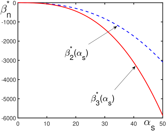
Figure 3: Gell-Mann-Low function of quantum chromodynamics for the flavour number $n_{f}=6$ as a function of the coupling parameter $\alpha_{s}$.

We are not aware of other reliable estimates of these characteristics that could be compared with our result for the physically interesting case of the flavour number $n_{f}=6$. The behaviour of the Gell-Mann-Low function of quantum chromodynamics for this flavour number, as a function of the coupling parameter, is shown in Fig. 3. For varying $n_{f}$, the Banks-Zaks [74] fixed point exists in the region $8.05\leq n_{f}\leq 16.5$.

The running coupling, defined by Eq. (54), with the boundary condition $\alpha_{s}(m_{Z})=0.1181$ logarithmically grows when $\mu$ tends to $\mu_{c}=0.1$ GeV from above,

$$\alpha_{s}\simeq\frac{0.907}{(\ln(\mu/\mu_{c}))^{0.626}}\qquad(\mu\rightarrow\mu_{c}+0)\;.$$

The appearance of a pole at $\mu_{c}$ characterizes the scale at which perturbative QCD breaks down, so that the series (55) as such, and hence their extrapolation, become invalid. The value of $\mu_{c}$ can be associated with the confinement scale, or equivalently the hadronic mass scale and nonperturbative effects, such as the arising bound states [70]. The smaller the value of $\mu_{c}$, i.e., the smaller the momentum scale at which the divergence occurs, the slower the increase of $\alpha_{s}(\mu)$ as $\mu$ decreases. This would imply the effective extrapolation of perturbative expressions to smaller momentum scales [70]. The value of $\mu_{c}$ is really much smaller than the point of the Landau pole which in the $(\overline{\rm MS})$ scheme for $n_{f}=6$ happens at the point $0.9$ GeV [75].

8 Discussion

In the above examples, we have considered the cases where the large-variable behavior is of power-law. As is demonstrated, for these cases, self-similar factor approximants can provide good extrapolation of small-variable Taylor-type asymptotic expansions to the range of finite variables and even for the large-variable limit. Moreover, in some cases these approximants, using only a small-variable expansion, are able to reconstruct the sought function exactly, as in the case of the Gell-Mann-Low function for the supersymmetric pure Yang-Mills theory and in some other cases to be considered below.

Two related natural questions arise: How well the self-similar factor approximants could extrapolate the functions with the large-variable behavior different from the power-law, such as exponential and logarithmic behavior? And the other question is: What would be other examples of the exact function reconstruction by means of self-similar factor approximants?

8.1 Class of exactly reproducible functions

First of all, let us notice that there exists a class of real-valued functions exactly reproducible by factor approximants. These are the functions having the form

$$R_{k_{M}}(x)=\prod_{i=1}^{M}\;P_{m_{i}}^{\alpha_{i}}(x)$$ (60)

of the product of polynomials

$$P_{m_{i}}(x)=c_{i0}+c_{i1}x+c_{i2}x^{2}+\cdots+c_{im_{i}}x^{m_{i}}\;,$$

where $m_{i}$ are integers; the powers $\alpha_{i}$ and coefficients $c_{ij}$ can be complex-valued numbers entering $R_{k_{M}}(x)$ in complex conjugate pairs so that $R_{k_{M}}(x)$ be real, and

$$k_{M}=\sum_{i=1}^{M}m_{i}+M.$$

This follows from the fact that a polynomial $P_{m_{i}}(x)$ can be represented as

$$P_{m_{i}}(x)=c_{i0}\prod_{j=1}^{m_{i}}\;(1+b_{ij}x)\;,$$

with $b_{ij}$ being expressed through $c_{ij}$. Then the function $R_{k_{M}}(x)$ can be reduced to the form

$$R_{k_{M}}(x)=\prod_{i=1}^{M}\;c_{i0}\;\prod_{j=1}^{m_{i}}\;(1+b_{ij}x)^{\alpha_{i}}\;,$$ (61)

which is nothing but a particular case of a factor approximant possessing the same asymptotic expansion as the given function (60).

If all powers $\alpha_{i}$ were $\pm 1$, then the function $R_{k}(x)$ would reduce to a Padé approximant that is a rational function. However the powers $\alpha_{i}$ are not necessarily integers. Hence factor approximants also include irrational functions that can be reproduced exactly.

8.2 Exact reconstruction of exponential functions

Moreover, factor approximants can exactly reproduce transcendental functions, such as the exponential function $\exp(x)$, where $x$ can take any complex value. Let us consider the standard $k$-order expansion of the exponential function

$$e_{k}(x)=\sum_{n=0}^{k}\frac{x^{n}}{n!}\;.$$ (62)

The second-order factor approximant is

$$e_{2}^{*}(x)=(1+Ax)^{n}\;.$$

Expanding this in powers of $x$ and comparing with $e_{k}(x)$ yields the equations

$$An=1\;,\qquad A^{2}n(n-1)=1\;.$$

The sole solution to these equations is $A=1/n$ with $n\rightarrow\infty$. Therefore already the second-order factor approximant gives exactly the exponential function

$$e_{2}^{*}(x)=\lim_{n\rightarrow\infty}\;\left(1+\frac{1}{n}\;x\right)^{n}=e^{x}\;.$$ (63)

It is easy to check that all factor approximants of the order $k\geq 2$ reconstruct the exponential function exactly.

8.3 Exact solution of nonlinear equations

Some nonlinear differential equations can be solved exactly by looking for solutions in the form of asymptotic series and then constructing factor approximants. For instance, let us consider the nonlinear singular problem

$$(\varepsilon y+t)\;\frac{dy}{dt}+y-1=0$$ (64)

with the initial condition $y(0)=2$. This kind of equation is met in different applications [76, 77]. It is called singular since it does not allow for the use of perturbation theory in powers of the parameter $\varepsilon$.

The parameter $\varepsilon$ can be hidden in the renotation

$$t=\varepsilon x\;,\qquad y=z-x$$

resulting in the equation

$$z\;\frac{dz}{dt}-x-1=0\;,$$

with the initial condition $z(0)=2$. Looking for the solution at asymptotically small $x$ implies the consideration of the series

$$z_{k}(x)=\sum_{n=0}^{k}a_{n}x^{n}\;,$$

whose coefficients can be found by substituting these series into the equation. Thus $a_{0}=2$, $a_{1}=1/2$, $a_{3}=3/16$, and so on. Constructing the fourth-order factor approximant gives

$$z_{4}^{*}(x)=2(1+A_{1}x)^{n_{1}}(1+A_{2}x)^{n_{2}}\;,$$

with the parameters

$$A_{1}=\frac{1}{4}\;(1-i\sqrt{3})=A_{2}^{*}\;,\qquad n_{1}=n_{2}=\frac{1}{2}\;.$$

Returning to the initial variables yields the function

$$y_{4}^{*}(t)=\sqrt{4+\frac{2t}{\varepsilon}+\frac{t^{2}}{\varepsilon^{2}}}\;-\;\frac{t}{\varepsilon}$$ (65)

that is the exact solution of the given equation. The same exact solution results for any factor approximant of $k\geq 4$.

Exact solutions of several other nonlnear differential equations can also be found by employing the summation of asymptotic series by means of the self-similar factor approximants [78].

8.4 Exponential behavior: Bose-Einstein distribution

As is shown above, the purely exponential behavior is reproduced by factor approximants exactly. Then we should expect that a behavior close to the purely exponential could be well approximated by these approximants. Let us consider the well known Bose-Einstein distribution

$$f_{B}(x)=\frac{1}{e^{x}-1}\;.$$ (66)

Suppose, only the expansion at small $x$,

$$f_{B}(x)\simeq\frac{1}{x}\;-\;\frac{1}{2}\;+\;\frac{x}{12}\;-\;\frac{x^{3}}{720}\;+\;\frac{x^{5}}{30240}\;-\;\frac{x^{7}}{1209600}\;+\;\ldots\qquad(x\rightarrow 0)\;,$$ (67)

is available for us, and we do not know what function it represents.

In the standard way, we construct factor approximants $f_{k}^{*}(x)$ that extrapolate expansion (67) from asymptotically small $x$ to finite values of the latter. Our major interest is in the approximants providing the extrapolation to the large variable behavior with respect to $x\rightarrow\infty$. By their structure, the factor approximants give the power-law behavior at infinity, for instance

$$f_{4}^{*}(x)\simeq 2.94\cdot\frac{10^{-3}}{x^{3}}\;,\qquad f_{8}^{*}(x)\simeq 1.1\cdot\frac{10^{-7}}{x^{5}}\;,\qquad f_{12}^{*}(x)\simeq 2.97\cdot\frac{10^{-14}}{x^{7}}\qquad(x\rightarrow\infty)\;.$$

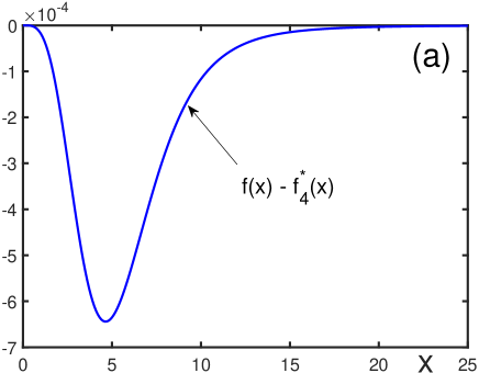
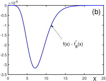
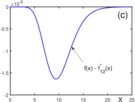
Figure 4: Difference between the Bose-Einstein distribution (66) and its self-similar factor approximants: (a) $f_{B}(x)-f_{4}^{*}(x)$; (b) $f_{B}(x)-f_{8}^{*}(x)$; (c) $f_{B}(x)-f_{12}^{*}(x)$.

As we see, these values quickly diminish, telling us that the real behavior at large $x$ is faster then of power law, probably, of exponential type. If we expect that the large-variable behavior is exponential, we can employ another variant of self-similar approximants, i.e. the self-similar exponential approximants [79]. However, since, as is proved above, the factor approximants well approximate the exponential behavior, they should provide rather good accuracy for the extrapolation of the distribution (45), which is demonstrated in Fig. 4. The exact Bose-Einstein distribution (66) and its factor approximants practically coincide in a large range of $x$, because of which in Fig. 4 we show their difference.

8.5 Exponential behavior: Fermi-Dirac distribution

Similarly, we can consider the Fermi-Dirac distribution

$$f_{F}(x)=\frac{1}{e^{x}+1}\;.$$ (68)

Again assume that we possess only the small-variable expansion

$$f_{F}(x)\simeq\frac{1}{2}\;-\;\frac{x}{4}\;+\;\frac{x^{3}}{48}\;-\;\frac{x^{5}}{480}\;+\;\frac{17x^{7}}{80640}\;-\;\frac{31x^{9}}{1451520}\;+\;\ldots\qquad(x\rightarrow 0)$$ (69)

and are not aware of the function it corresponds to. Factor approximants $f_{k}^{*}(x)$ that extrapolate the series (69) to the large-variable range again quickly diminish, for instance

$$f_{4}^{*}(x)\simeq 6.7\cdot\frac{10^{-2}}{x^{2}}\;,\qquad f_{8}^{*}(x)\simeq 3.4\cdot\frac{10^{-5}}{x^{4}}\;\qquad f_{12}^{*}(x)\simeq 1.05\cdot\frac{10^{-10}}{x^{6}}\qquad(x\rightarrow\infty)\;.$$

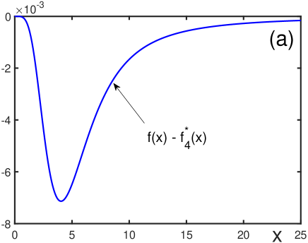
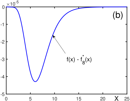
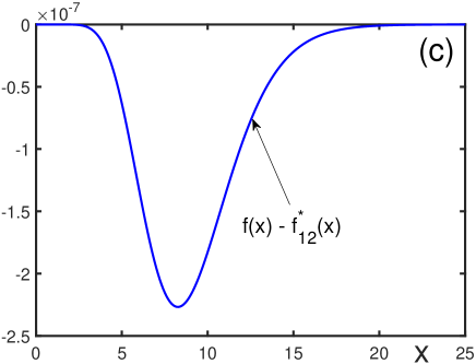
Figure 5: Difference between the Fermi-Dirac distribution (68) and its self-similar factor approximants: (a) $f_{F}(x)-f_{4}^{*}(x)$; (b) $f_{F}(x)-f_{8}^{*}(x)$; (c) $f_{F}(x)-f_{12}^{*}(x)$.

This hints that the large-variable behavior should be faster than of power law. Nevertheless, since factor approximants well approximate the purely exponential behavior, they should provide quite accurate approximation for the considered distribution. Again, the exact distribution (68) and its factor approximants practically coincide in a large region of $x$, because of which in Fig. 5 the related differences are shown.

8.6 Logarithmic behavior: no additional information

Now let us turn to functions with logarithmic asymptotic behavior at large values of a variable. Let us take the function

$$f(x)=1+\ln\;\left(\frac{1+\sqrt{1+x}}{2}\right)\;,$$ (70)

with the logarithmic asymptotic behavior at large $x$,

$$f(x)\simeq\frac{1}{2}\ln\;x\qquad(x\rightarrow\infty)\;.$$ (71)

Let us pretend that we know neither the function itself nor its behavior at large $x$, but what available is only the asymptotic expansion at small $x$,

$$f(x)\simeq 1\;+\;\frac{1}{4}\;x\;-\;\frac{3}{32}\;x^{2}\;+\;\frac{5}{96}\;x^{3}\;-\;\frac{35}{1024}\;x^{4}\;+\;\frac{63}{2560}\;x^{5}\;-\;\frac{77}{4096}\;x^{6}\;+\ldots\qquad(x\rightarrow 0)\;.$$ (72)

Constructing factor approximants from these series, we find that their large-variable behavior demonstrates not so fast variation of the amplitude and power:

$$f_{2}^{*}(x)\simeq x^{0.25}\;,\qquad f_{4}^{*}(x)\simeq 1.195\;x^{0.182}\;,\qquad f_{6}^{*}(x)\simeq 1.137\;x^{0.197}\;,$$

$$f_{8}^{*}(x)\simeq 1.237\;x^{0.1747}\;,\qquad f_{10}^{*}(x)\simeq 1.235\;x^{0.1749}\;,\qquad f_{12}^{*}(x)\simeq 1.310\;x^{0.162}\qquad(x\rightarrow\infty)\;.$$

Although, as is typical of the factor approximants, the large-variable dependence is of power law, the factor approximants provide reasonable accuracy in a wide region of the variable $x$, as is seen in Fig. 6(a).

8.7 Logarithmic behavior: known character of large-variable limit

A different situation develops when, although the function itself is not known, but there is information that the large-variable behavior is expected to be logarithmic. Then it is reasonable to deal not with series (72), but with the exponential of it. This implies that a finite series $f_{k}(x)$, corresponding to the truncated series (72), is exponentiated considering

$$g_{k}(x)=\exp\{f_{k}(x)\}$$ (73)

and then expanding the latter up to the $k$-th order. In the case of series (72), we have

$$g(x)\simeq e\left(1+\frac{1}{4}\;x\;-\;\frac{1}{16}\;x^{2}\;+\;\frac{1}{32}\;x^{3}\;-\;\frac{5}{256}\;x^{4}\;+\;\frac{7}{512}\;x^{5}\;-\;\frac{21}{2048}\;x^{6}\;+\;\ldots\;\right)\quad(x\rightarrow 0)\;.$$ (74)

The latter series is used for constructing the factor approximants $g_{k}^{*}(x)$, after which, inverting transformation (73), we return to the expressions

$$F_{k}^{*}(x)=\ln\;g_{k}^{*}(x)$$ (75)

approximating the sought function. Here we denote the final approximants as $F_{k}^{*}(x)$ to distinguish them from the approximants $f_{k}^{*}(x)$ obtained directly from series (72).

The large-variable behavior of the approximants $F_{k}^{*}(x)$ is of correct logarithmic form, for example

$$F_{2}^{*}(x)\simeq 0.333\ln x\;,\qquad F_{4}^{*}(x)\simeq 0.4\ln x\;,\qquad F_{6}^{*}(x)\simeq 0.429\ln x\;,$$

$$F_{8}^{*}(x)\simeq 0.444\ln x\;,\qquad F_{10}^{*}(x)\simeq 0.456\ln x\;,\qquad F_{12}^{*}(x)\simeq 0.462\ln x\qquad(x\rightarrow\infty)\;.$$

The coefficient at the logarithm converges to the exact value $0.5$, in agreement with limit (71). The overall behavior of the approximants $F_{k}^{*}(x)$ is shown in Fig. 6(b). As it should be expected, the additional information on the behavior of the function essentially improves the accuracy of the approximation.

9 Conclusion

We have suggested a method, based on self-similar approximation theory, allowing for the extrapolation of expressions from weak-coupling asymptotic expansions to the region of arbitrary values of coupling parameters, including their asymptotically large values. The region of large coupling parameters is of special interest because of its physical importance and because mathematically this region is the most difficult for the extrapolation that uses only the coefficients of weak-coupling expansions.

In those cases, where a number of terms in the small-variable expansion are available, the method is shown to posses numerical convergence. Good accuracy can be obtained even for the expansions with a few terms. The extrapolation of perturbative series for the Gell-Mann-Low functions of the $O(N)$ symmetric $\varphi^{4}$ field theory, quantum electrodynamics, and quantum chromodynamics is demonstrated.

In some cases, the method can transform perturbative series to the exact expression valid for arbitrary values of the variable. Such an exact reconstruction is illustrated for the Gell-Mann-Low function of a supersymmetric pure Yang-Mills theory and for several other examples.

By their construction, self-similar factor approximants, for the variable tending to infinity, give a power-law behavior. The possibility is discussed of extrapolating functions with different types of the large-variable limits, including not only power-law behavior, but also logarithmic and exponential behavior. The purely exponential function is shown to be reconstructed exactly by the factor approximants of any order starting from second. More complicated functions with exponential or logarithmic large-variable behavior can be well approximated in a wide range of the variable. If the additional information on the character of the large-variable limit is available, the accuracy of the approximants can be essentially improved.

Figure Captions

Figure 1. Gell-Mann-Low function of $\varphi^{4}$ $O(1)$ symmetric field theory as a function of the coupling parameter $g$. The convergence of the approximants of second, fourth, and sixth order is evident.

Figure 2. Gell-Mann-Low function of quantum electrodynamics as a function of the coupling parameter $\alpha$.

Figure 3. Gell-Mann-Low function of quantum chromodynamics for the flavour number $n_{f}=6$ as a function of the coupling parameter $\alpha_{s}$.

Figure 4. Difference between the Bose-Einstein distribution (66) and its self-similar factor approximants: (a) $f_{B}(x)-f_{4}^{*}(x)$; (b) $f_{B}(x)-f_{8}^{*}(x)$; (c) $f_{B}(x)-f_{12}^{*}(x)$.

Figure 5. Difference between the Fermi-Dirac distribution (68) and its self-similar factor approximants: (a) $f_{F}(x)-f_{4}^{*}(x)$; (b) $f_{F}(x)-f_{8}^{*}(x)$; (c) $f_{F}(x)-f_{12}^{*}(x)$.

Figure 6. (a) Function (70) (solid line) and its self-similar factor approximants obtained from the direct series (72): $f_{4}^{*}(x)$ (dotted line), $f_{8}^{*}(x)$ (dash-dotted line), and $f_{12}^{*}(x)$ (dashed line). (b) Function (70) (solid line) and its self-similar factor approximants obtained from expansion (74): $F_{4}^{*}(x)$ (dotted line), $F_{8}^{*}(x)$ (dash-dotted line), and $F_{12}^{*}(x)$ (dashed line).

         

         

         

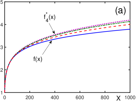
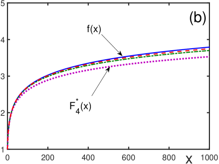
Figure 6: (a) Function (70) (solid line) and its self-similar factor approximants obtained from the direct series (72): $f_{4}^{*}(x)$ (dotted line), $f_{8}^{*}(x)$ (dash-dotted line), and $f_{12}^{*}(x)$ (dashed line). (b) Function (70) (solid line) and its self-similar factor approximants obtained from expansion (74): $F_{4}^{*}(x)$ (dotted line), $F_{8}^{*}(x)$ (dash-dotted line), and $F_{12}^{*}(x)$ (dashed line).

References

- [1] G.A. Baker and P. Graves-Moris, Padé Approximants (Cambridge University Press, Cambridge, 1996).
- [2] G.A. Baker and J.L. Gammel, The Padé approximant, J. Math. Anal. Appl. 2, 21–30 (1961).
- [3] G.H. Hardy, Divergent Series (Chelsea, Rhode Island, 1992).
- [4] H. Kleinert, Path Integrals (World Scientific, Singapore, 2003).
- [5] S. Weinberg, The Quantum Theory of Fields (Cambridge University Press, Cambridge, 2005).
- [6] O. Costin and G.V. Dunne, Resurgent extrapolation: Rebuilding a function from asymptotic data, Painlevé I, J. Phys. A 52, 445205 (2019).
- [7] O. Costin and G.V. Dunne, Physical resurgent extrapolation, Phys. Lett. B 808, 135627 (2020).
- [8] O. Costin and G.V. Dunne, Uniformization and constructive analytic continuation of Taylor series, arXiv:2009.01962 (2020).
- [9] V.I. Yukalov, Theory of perturbations with a strong interaction, Moscow Univ. Phys. Bull. 31, 10–15 (1976).
- [10] V.I. Yukalov, Model of a hybrid crystal, Theor. Math. Phys. 28, 652–660 (1976).
- [11] V.I. Yukalov, Quantum crystal with jumps of particles, Physica A 89, 363–372 (1977).
- [12] V.I. Yukalov, Quantum theory of localized crystal, Ann. Phys. (Berlin) 491, 31–39 (1979).
- [13] W.E. Caswell, Accurate energy levels for the anharmonic oscillator and a summable series for the double well potential in perturbation theory, Ann. Phys. (N.Y.) 123, 153–184 (1979).
- [14] I.G. Halliday and P. Suranyi, Anharmonic oscillator: A new approach, Phys. Rev. D 21, 1529–1537 (1980).
- [15] J. Killingbeck, Renormalized perturbation series, J. Phys. A 14, 1005–1008 (1981).
- [16] P.M. Stevenson, Optimized perturbation theory, Phys. Rev. D 23, 2916–2944 (1981).
- [17] I.D. Feranchuk and L.I.Komarov, The operator method of the approximate solution of the Schrödinger equation, Phys. Lett. A 88, 211–214 (1982).
- [18] V.I. Yukalov and V.I. Zubov, Localized-particles approach for classical and quantum crystals, Fortschr. Phys. 31, 627–672 (1983).
- [19] M. Dineykhan, G.V. Efimov, G. Gandbold, and S.N. Nedelko, Oscillator Representation in Quantum Physics (Springer, Berlin, 1995).
- [20] A.N. Sissakian and I.L. Solovtsov, Variational expansions in quantum chromodynamics, Phys. Part. Nucl. 30, 1057–1119 (1999).
- [21] H. Kleinert and V.I. Yukalov, Self-similar variational perturbation theory for critical exponents, Phys. Rev. E 71, 026131 (2005).
- [22] I. Feranchuk, A. Ivanov, V.H. Le, and A. Ulyanenkov, Nonperturbative Description of Quantum Systems (Springer, Cham, 2015).
- [23] B.S. Shaverdyan and A.G. Ushveridze, Convergent perturbation theory for the scalar field theories: The Gell-Mann-Low function, Phys. Lett. B 123, 316–318 (1983).
- [24] A.G. Ushveridze, Superconvergent perturbation theory for Eucledean scalar field theories, Phys. Lett. B 142, 403–406 (1984).
- [25] A.V. Turbiner and A.G. Ushveridze, Anharmonic oscillator: Constructing the strong coupling expansions, J. Math. Phys. 29, 2053–2063 (1988).
- [26] V. Sazonov, Convergent series for polynomial lattice models with complex actions, Mod. Phys. Lett. A 34, 1950243 (2019).
- [27] V.I. Yukalov and E.P. Yukalova, Degenerate trajectories and Hamiltonian envelopes in the method of self-similar approximations, Can. J. Phys. 71, 537–546 (1993).
- [28] S. Gluzman and V. I. Yukalov, Self-similarly corrected Padé approximants for the indeterminate problem, Eur. Phys. J. Plus. 131, 340 (2016).
- [29] S. Gluzman and V. I. Yukalov, Self-similarly corrected Padé approximants for nonlinear equations, Int. J. Mod. Phys. B 33, 1950353 (2019).
- [30] V.I. Yukalov, Statistical mechanics of strongly nonideal systems, Phys. Rev. A 42, 3324–3334 (1990).
- [31] V.I. Yukalov, Self-similar approximations for strongly interacting systems, Physica A 167, 833–860 (1990).
- [32] V.I. Yukalov, Method of self-similar approximations, J. Math. Phys. 32, 1235–1239 (1991).
- [33] V.I. Yukalov, Stability conditions for method of self-similar approximations, J. Math. Phys. 33, 3994–4001 (1992).
- [34] V.I. Yukalov and E.P. Yukalova, Self-similar perturbation theory, Ann. Phys. (N.Y.) 277, 219–254 (1999).
- [35] V.I. Yukalov and S. Gluzman, Self-similar interpolation in high-energy physics, Phys. Rev. D 91, 125023 (2015).
- [36] L.R. Foulds, Optimization Techniques (Springer, New York, 1981).
- [37] L.M. Hocking, Optimal Control (Clarendon, Oxford, 1991).
- [38] V.I. Yukalov and E.P. Yukalova, Self-similar structures and fractal transforms in approximation theory, Chaos Solit. Fract. 14, 839–861 (2002).
- [39] A.H. Cliffordand G.B. Preston, The Algebraic Theory of Semigroups (American Mathematical Society, Providence, 1967).
- [40] S. Lang, Algebra (Addison-Wesley, Reading, 1984).
- [41] M.F. Barnsley, Fractal Transform (AK Peters Ltd., Natick, 1994).
- [42] V.I. Yukalov, S. Gluzman, and D. Sornette, Summation of power series by self-similar factor approximants, Physica A 328, 409–438 (2003).
- [43] S. Gluzman, V.I. Yukalov, and D. Sornette, Self-similar factor approximants, Phys. Rev. E 67, 026109 (2003).
- [44] V.I. Yukalov and E.P. Yukalova, Calculation of critical exponents by self-similar factor approximants, Eur. Phys. J. B 55, 93–99 (2007).
- [45] N.J. Higham, Accuracy and Stability of Numerical Algorithms (SIAM, Philadelphia, 2002).
- [46] V.I. Yukalov and E.P. Yukalova, Describing phase transitions in field theory by self-similar approximants, Eur. Phys. J. Web Conf. 204, 02003 (2019).
- [47] C.M. Bender and T.T. Wu, Anharmonic oscillator, Phys. Rev. 184, 1231–1260 (1969).
- [48] F.T. Hioe, D. MacMillen, and E.W. Montroll, Quantum theory of anharmonic oscillators: Energy levels of a single and a pair of coupled oscillators with quartic coupling, Phys. Rep. 43, 305–335 (1978).
- [49] J. Schwinger, Gauge invariance and mass, Phys. Rev. 128, 2425–2428 (1962).
- [50] T. Banks, L. Susskind, and J. Kogut, Strong-coupling calculations of lattice gauge theories: -dimensional exercises, Phys. Rev. D 13, 1043–1053 (1976).
- [51] A. Carrol, J. Kogut, D.K. Sinclair, and L. Susskind, Lattice gauge theory calculations in dimensions and the approach to the continuum limit, Phys. Rev. D 13, 2270–2277 (1976).
- [52] J.P. Vary, T.J. Fields, and H.J. Pirner, Chiral perturbation theory in the Schwinger model, Phys. Rev. D 53, 7231–7238 (1996).
- [53] C. Adam, The Schwinger mass in the massive Schwinger model, Phys. Lett. B 382, 383–388 (1996).
- [54] P. Striganesh, C.J. Hamer, and R.J. Bursill, A new finite-lattice study of the massive Schwinger model, Phys. Rev. D 62, 034508 (2000).
- [55] C.J. Hamer, Z. Weihong, and J. Oitmaa, Series expansions for the massive Schwinger model in Hamiltonian lattice theory, Phys. Rev. D 56 , 55–67 (1997).
- [56] S. Coleman, More about the massive Schwinger model, Ann. Phys. (N.Y.) 101, 239–267 (1976).
- [57] C.J. Hamer, Lattice model calculations for SU(2) Yang-Mills theory in -dimensions, Nucl. Phys. B 121, 159–175 (1977).
- [58] V.A. Novikov, M.A. Shifman, A.I. Vainshtein, and V.I. Zakharov, Exact Gell-Mann-Low function of supersymmetric Yang-Mills theories from instanton calculus, Nucl. Phys. B 229, 381–393 (1983).
- [59] V.A. Novikov, M.A. Shifman, A.I. Vainshtein, and V.I. Zakharov, The beta function in supersymmetric gauge theories: Instantons versus traditional approach, Phys. Lett. B 166, 329–333 (1986).
- [60] M.A. Shifman and A.I. Vainshtein, Solution of the anomaly puzzle in SUSY gauge theories and the Wilson operator expansion, Nucl. Phys. B 277, 456–486 (1986).
- [61] N. Arkani-Hamed and H. Murayama, Renormalization group invariance of exact results in supersymmetric gauge theories, Phys. Rev. D 57, 6638–6648 (1998).
- [62] N. Arkani-Hamed and H. Murayama, Holomorphy, rescaling anomalies and exact functions in supersymmetric gauge theories, J. High Energy Phys. 2000, 030 (2000).
- [63] I.O. Goriachuk and A.L. Kataev, Exact -function in Abelian and non-Abelian supersymmetric gauge models and its analogy with the QCD -function in the C-scheme, JETP Lett. 111, 663–667 (2020).
- [64] M.V. Kompaniets and E. Panzer, Minimally subtracted six-loop renormalization of -symmetric theory and critical exponents, Phys. Rev. D 96, 036016 (2017).
- [65] O. Schnetz, Numbers and functions in quantum field theory, Phys. Rev. D 97, 085018 (2018).
- [66] D.I. Kazakov, O.V. Tarasov, and D.V. Shirkov, Analytic continuation of the results of perturbation theory for the model to the region , Theor. Math. Phys. 38, 9–16 (1979).
- [67] K.G. Chetyrkin, S.G. Gorishny, S.A. Larin, and F.V. Tkachev, Five-loop renormalization group calculations in the theory, Phys. Lett. B 132, 351–354 (1983).
- [68] A.N. Sissakian, I.L. Solovtsov, and O.P. Solovtsova, -function for the -model in variational perturbation theory, Phys. Lett. B 321, 381–384 (1994).
- [69] A.L. Kataev and S.A. Larin, Analytical five-loop expressions for the renormalization group QED -function in different renormalization schemes, JETP Lett. 96, 61–65 (2012).
- [70] A. Deur, S.J. Brodsky, and G.F. de Teramond, The QCD running coupling, Prog. Part. Nucl. Phys. 90, 1–74 (2016).
- [71] T. Luthe, A. Maier, P. Marquard, and Y. Schröder, Towards the five-loop beta function for a general gauge group, J. High Energy Phys. 2016, 127 (2016).
- [72] P.A. Baikov, K.G. Chetyrkin, and J.H. Kühn, Five-loop running of the QCD coupling constant, Phys. Rev. Lett. 118, 082002 (2017).
- [73] F. Herzog, B. Ruijl, T. Ueda, J.A.M. Vermaseren, and A. Vogt, The five-loop beta function of Yang-Mills theory with fermions, J. High Energy Phys. 2017, 090 (2017).
- [74] T. Banks and A. Zaks, On the phase structure of vector-like gauge theories with massless fermions, Nucl. Phys. B 196, 189–204 (1982).
- [75] M. Tanabashi et al., Review of particle physics (Particle Data Group), Phys. Rev. D 98, 030001 (2018).
- [76] A.H. Nayfeh, Perturbation Methods (Wiley, New York, 1973).
- [77] E.J. Hinch, Perturbation Methods (Cambridge University, Cambridge, 1991).
- [78] E.P. Yukalova, V.I. Yukalov, and S. Gluzman, Self-similar factor approximants for evolution equations and boundary-value problems, Ann. Phys. (N.Y.) 323, 3074–3090 (2008).
- [79] V.I. Yukalov ans S. Gluzman, Self-similar exponential approximants, Phys. Rev. E 58, 1359–1382 (1998).