Particle acceleration around rotating Einstein-Born-Infeld black hole and plasma effect on gravitational lensing

Abstract

We consider a time-like geodesics in the background of rotating Einstein-Born-Infeld (EBI) black hole to examine the horizon and ergosphere structure. The effective potential that governs the particle’s motion in the spacetime and the innermost stable circular orbits (ISCO) is also studied. A qualitative analysis is conducted to find the redshifted ultrahigh centre-of-mass (CM) energy as a result of a two-particle collision specifically near the horizon. The recent Event Horizon Telescope (EHT) triggered a surge of interest in strong gravitational lensing by black holes, which provide a new tool comparing the black hole lensing in general relativity and alternate gravity theories. Motivated by this, we also discussed both strong and weak-field gravitational lensing in the space-time discretely for a uniform plasma and a singular isothermal sphere. We calculated the light deflection coefficients $\bar{a}$ and $\bar{b}$ in the strong field limits, and their variance with the rotational parameter $a$ for different plasma frequency as well as in vacuum. For EBI black holes, we found that plasma’s presence increases the photon sphere radius, the deflection angle, the deflection coefficients $\bar{a}$, $\bar{b}$, the angular positions and the angular separation between the relativistic images. It is also shown that with increasing spin the impact of plasma on a strong gravitational lensing becomes smaller as the spin parameter grows in the prograde orbit ($a>0$). For extreme black holes, the strong gravitational effects in the homogenous plasma are similar to those of in a vacuum. We investigate strong gravitational lensing effects by supermassive black holes Sgr A* and M87*. Considering rotating EBI black holes as the lens, we find the angular position of images for Sgr A* and M87* and observe that the deviations of the angular position from that of the analogous Kerr black hole are not more than $2.44~{}\mu$as for Sgr A* and $1.83~{}\mu$as for M87*, which are unlikely to get resolved by the current EHT observations.

I Introduction

The existence of black holes has remained a subject of interest ever since Einstein discovered their presence in the Universe with General Relativity’s theory. The black holes were believed to form when the matter in space experienced a cataclysmic collapse and eventually reduced to a singular point, where both the density and curvature of the spacetime approach to infinity. However, this theory could not convince the presence of black holes on observational level, because of this misconception Roger Penrose proposed the Cosmic censorship conjecture, which assuredly denies the existence of the naked singularities. According to the latter theory the event horizon is an integral part of the singularity. Theoretical beliefs are whatsoever incomplete unless backed up by the observational results, therefore the probe to visualize a black hole has recently become possible in 2019 by the Event Horizon Telescope (EHT) collaboration aki:2019a ; aki:2019b .

Penrose unveiled that the black holes can also serve as an energy source to the matter in its surroundings Penrose:1971a . Quite a lot lately, Bandos, Silk, and West (BSW) explored that the Kerr black holes could provide a platform to the accelerated particles for a collision to obtain a ultrahigh energy near the horizon Bds:2009a . Up till now, an extensive research has been done in analogy to the BSW mechanism for different gravities Zasl:2010a ; Grib:2011a ; Zasl:2012a ; Zasl:2012b ; Zasl:2012c ; Turs:2013a ; Shay:2013a ; Zasl:2013aa ; Far:2013aa ; Abu:2015e . In some of the noteworthy articles Wei:2011a ; Abu:2011c ; Abu:2013c ; Josh:2015a ; Amir:2015pja ; Ghosh:2014mea ; Zhang:2019a the authors studied the BSW effect in backgrounds of Kerr-Newman, Ho$\mathrm{\hat{r}}$ava-Lifshitz, five-dimensional Kerr black hole, Bardeen space-time, Kerr–de Sitter and Kerr–anti– de Sitter black holes, correspondingly. Considering the Kerr spacetime, Harada Harada:2011a investigated the CM energies resulting from a collision between two particles in the ISCO. Although the controversial arguments still exist about the naked singularities, nevertheless Patil and Joshi researched the CM energies in the surroundings of naked singularities patail:2012a ; patail:2012b and surprisingly, succeeded to achieve a large amount of energy near the singularities. Later on, Stuchlík et al. explored ultra-high energy collisions in the vicinity of Kehagias-Sfetsos gravityStuc:2014a . Most recently, the CM energy generated in various spacetimes are addressed in the articles Vrba:2019a ; Hejda:2019a ; Ray:2020a ; Abu:2020e .

The black hole gravity allows several paranormal astrophysical activities in its surroundings, wherein gravitational lensing is one of them. Assuming a strong-field regime Virbhadra and Ellis analysed the null-geodesics in Virbha:2000a , which in fact made an unprecedented contribution to the exploration of black holes with a unique approach. The authors also extended their work for naked singularities in Virbha:2002a . Bozza et al. employed analytical technique in Bozza:2001aa ; Bozza:2002b to study the properties of strong-field lensing. Furthermore, some of the interesting additions which analysed this specific field efficiently are provided in Bozza:2003a ; Sevb:2004a ; Bozza:2005a ; Bozza:2006a ; Eiroa:2002b ; Eiroa:2004a ; Eiroa:2005a ; Wei:2012b ; Eiroa:2014a ; Sotani:2015a ; Zhao:2017a . So far, this event has been studied by many astrophysicists predominantly for the black holes surrounded by a plasma, however, Bisnovatyi-Kogan and Tsupko have played a significant role in the investigations Bin:2010a ; Tsp:2011a ; Tsp:2014a ; Tsp:2015a . In accordance with the aforesaid analysis references Abu:2013a ; Atamurotov:2021a ; Rog:2015a ; Islam:2020xmy ; Kumar:2020sag ; Ghosh:2020spb ; Far:2016a ; Bis:2017a ; Abu:2017aa ; Abu:2017a ; Car:2018a ; Chak:2018a ; Turi:2019a ; Babar:2020a yield compelling details for various gravitational spacetimes.

In this paper our main interest is to examine the time-like and null geodesics in the rotating Einstein-Born-Infeld (EBI) spacetime to retrace the BSW effect along with the strong and weak-field gravitational lensing, respectively. Before the EBI gravity came into acknowledgment, it was Born and Infeld Born:1934a who primarily introduced the nonlinear electromagnetic field in the classical electrodynamics which was afterwards coupled with the general relativity by Hoffmann Hoff:1935a to obtain a spherically symmetric solution for the gravitational field of an electrically charged object. The EBI gravity received well acclaim when the Born–Infeld type actions appeared consecutively Frad:1985a ; Berg:1987a ; Mets:1987a in the light of low energy string theory. We can get a productive understanding of the EBI spacetime from the research articles Demi:1986a ; Gibb:1995a ; Gibb:1996b ; DP:1997a ; Chr:2000a ; Feig:1998a ; Feig:1998b ; Fernan:2003a ; Comel:2005a ; Comel:2004a ; Nieto:2004a ; Wohl:2004a , regarding its optimal solution and distinct features.

The rest of our paper is structured as follows. Sec. (II) incorporates the analysis of generic features of the black hole mainly the horizons and the ergosphere region. In Sec. (III) the effective potential in tandem with the center-of-mass energy of collision between two identical particles is thoroughly examined. Sec. (IV) sheds light on the gravitational lensing phenomenon in a strong-field regime distinctively for the vacuum and plasma backgrounds along with the corresponding observables. Sec. (V) renders an elaborate analysis of the deflection angle caused by the deviation of photons in a weak-field approximation considering two separate cases of the medium surrounding the black hole, i.e, a uniform plasma and a singular isothermal sphere. Finally, in Sec. (VI) we briefed about the main results.

II Geodesic of rotating EBI black holes

The action which leads to the field equations of EBI gravity is obtained when the gravitational field is coupled to a nonlinear Born–Infeld electrodynamics Born:1934a in $(3+1)$ dimensions Hoff:1935a reads

$$I=\bigintssss d^{4}x\sqrt{-g}\Bigg{(}\frac{R}{16\pi G}+\mathcal{L}(\mathcal{F})\Bigg{)},$$ (1)

where $R$ is the scalar curvature and $g=\mathrm{det}|g_{\mu\nu}|$. The Lagrangian $\mathcal{L}(\mathcal{F})$ is defined as

$$\mathcal{L}(\mathcal{F})=\frac{\beta^{2}}{4\pi G}\Bigg{(}1-\sqrt{1+\frac{2\mathcal{F}}{\beta^{2}}}\Bigg{)}.$$ (2)

$\mathcal{F}=\frac{1}{4}F_{\mu\nu}F^{\mu\nu}$, $F_{\mu\nu}$ indicates the electromagnetic field tensor. The symbol $\beta$ is the Born–Infeld parameter, equal to the maximum value of electromagnetic field intensity. The Einstein field equations and the electromagnetic field equations are constructed out of (1), respectively, as

$$R_{\mu\nu}-\frac{1}{2}g_{\mu\nu}R=kT_{\mu\nu},$$ (3)

$$\nabla_{\mu}(F^{\mu\nu}\mathcal{L}_{,\mathcal{F}})=0.$$ (4)

The energy-momentum $T_{\mu\nu}$ reads

$$T_{\mu\nu}=\mathcal{L}g_{\mu\nu}-F_{\mu\eta}F^{\eta}_{\nu}.$$ (5)

$\mathcal{L}_{,F}$ represents the partial derivative of $\mathcal{L}$ with respect to $\mathcal{F}$. The spacetime of a static and spherically symmetric compact object with mass $M$ and a nonlinear electromagnetic source in the EBI postulated theory has been foremostly investigated by Hoffmann Hoff:1935a . The metric for EBI space-time is expressed as Gibb:1995a ; Gibb:1996b ; DP:1997a ; Chr:2000a

$$ds^{2} =-f(r)dt^{2}+f(r)^{-1}dr^{2}+r^{2}(d\theta^{2}+\sin^{2}\theta d\phi^{2}),$$

$$f(r) =\bigg{(}1-\frac{2GM}{r}+\frac{Q^{2}(r)}{r^{2}}\bigg{)},$$ (6)

whereas, $Q^{2}(r)$ is a unique composition of the black hole’s charge $Q$, the Born-Infeld parameter $\beta$ and $r$.

$$Q^{2}(r)=\frac{2\beta^{2}r^{4}}{3}\bigg{(}1-\sqrt{1+\xi^{2}(r)}\bigg{)}$$

$$+\frac{4Q^{2}}{3}F\bigg{(}\frac{1}{4},\frac{1}{2},\frac{5}{4},-\xi^{2}(r)\bigg{)},$$ (7)

here, $F$ denotes the Gauss hypergeometric function and the parameter $\xi^{2}(r)$ is characterised by $\frac{Q^{2}}{\beta^{2}r^{4}}$. The rotating EBI metric is obtained by applying the Newman-Janis algorithm Newman:1965 to static spherical metric (II). The gravitational field of a rotating EBI black hole in the Boyer Lindquist coordinates is described by the line element Lomb:2004a ,

$$ds^{2} =-\bigg{(}\frac{\Delta-a^{2}\sin^{2}\theta}{\rho^{2}}\bigg{)}dt^{2}+\frac{\rho^{2}}{\Delta}dr^{2}+\rho^{2}d\theta^{2}$$

$$+\sin^{2}\theta\bigg{(}\rho^{2}+a^{2}\sin^{2}\theta\bigg{(}2-\frac{\Delta-a^{2}\sin^{2}\theta}{\rho^{2}}\bigg{)}\bigg{)}d\phi^{2}$$

$$-2a\sin^{2}\theta\bigg{(}1-\frac{\Delta-a^{2}\sin^{2}\theta}{\rho^{2}}\bigg{)}dtd\phi,$$ (8)

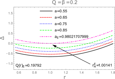
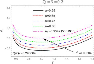
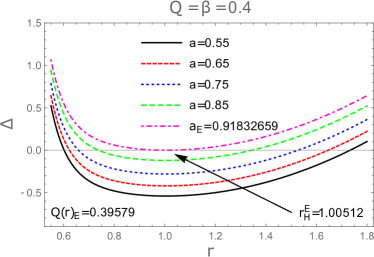
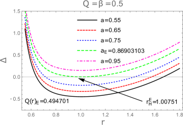
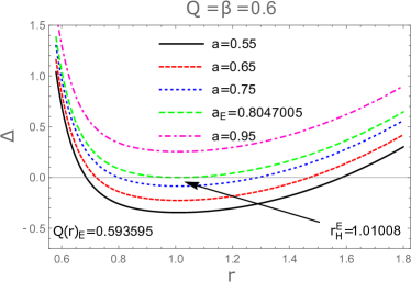
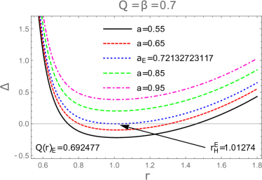
Figure 1: Plot showing the behavior of $\Delta$ with respect to $r$ for different values of $Q=\beta$. The case $a=a_{E}$ corresponds to an extremal black hole.

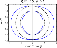
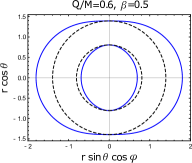
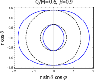
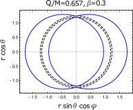
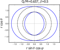
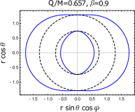
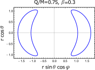
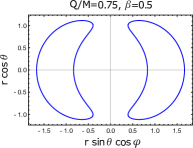
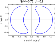
Figure 2: Plot showing the variation of the shape of ergosphere for a rotating charged black hole in $xz$-plane with a fixed spin parameter $a=0.7$ and for various charge $Q$ and Born-Infeld parameters $\beta$. The blue and the black lines correspond, respectively, to the static limit surfaces and horizons.

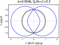
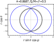
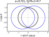
Figure 3: Plot showing the variation of the shape of ergosphere for $a\approx a_{E}$ (extremal black hole) in $xz$-plane with parameters $Q/M=\beta$, for a rotating EBI black hole.

Table 1: The values of the horizons of a rotating EBI black hole with $a$=0.5. The Kerr-Newman case is shown by $\beta\rightarrow\infty.$

Q	$\beta=0.4$				$\beta=0.6$				$\beta=0.8$				$\beta=1$				$\beta\rightarrow\infty$
	$r_{H}^{-}$		$r_{H}^{+}$		$r_{H}^{-}$		$r_{H}^{+}$		$r_{H}^{-}$		$r_{H}^{+}$		$r_{H}^{-}$		$r_{H}^{+}$		$r_{H}^{-}$		$r_{H}^{+}$
0.4	0.5945		1.7686		0.4977		1.7684		0.4403		1.7683		0.4012		1.7682		0.2319		1.7681
0.5	0.7000		1.7086		0.5851		1.7078		0.5174		1.7075		0.4717		1.7074		0.2929		1.7071
0.6	0.8085		1.6285		0.6746		1.6265		0.5969		1.6256		0.5451		1.6252		0.3755		1.6245
0.7	0.9289		1.5197		0.7728		1.5154		0.6849		1.5132		0.6275		1.5121		0.4901		1.5099
0.8	1.1001		1.3452		0.8984		1.3503		0.7985		1.3443		0.7378		1.3404		0.6683		1.3316

Table 2: The values of the outer static limit surface and event horizon of a rotating EBI black hole with $a$=0.5 and $\theta=\frac{\pi}{2}$ ($\delta_{e}^{g}$= $r_{sls}^{+}$ - $r_{H}^{+}$). The Kerr-Newman case is shown by $\beta\rightarrow\infty$.

Q	$\beta=0.4$				$\beta=0.6$				$\beta=0.8$				$\beta=1$				$\beta\rightarrow\infty$
	$r_{H}^{+}$	$r_{sls}^{+}$	$\delta_{e}^{g}$		$r_{H}^{+}$	$r_{sls}^{+}$	$\delta_{e}^{g}$		$r_{H}^{+}$	$r_{sls}^{+}$	$\delta_{e}^{g}$		$r_{H}^{+}$	$r_{sls}^{+}$	$\delta_{e}^{g}$		$r_{H}^{+}$	$r_{sls}^{+}$	$\delta_{e}^{g}$
0.4	1.7686	1.9168	0.1482		1.7684	1.9167	0.1483		1.7683	1.9166	0.1483		1.7682	1.9166	0.1484		1.7681	1.9165	0.1484
0.5	1.7086	1.8669	0.1583		1.7078	1.8664	0.1586		1.7075	1.8663	0.1588		1.7074	1.8662	0.1588		1.7071	1.8660	0.1589
0.6	1.6285	1.8022	0.1737		1.6265	1.8010	0.1745		1.6256	1.8006	0.1750		1.6252	1.8004	0.1752		1.6245	1.8000	0.1755
0.7	1.5197	1.7192	0.1995		1.5154	1.7167	0.2013		1.5132	1.7156	0.2024		1.5121	1.7151	0.2030		1.5099	1.7141	0.2042
0.8	1.3452	1.6111	0.2659		1.3503	1.6063	0.2560		1.3443	1.6038	0.2595		1.3404	1.6025	0.2621		1.3316	1.6000	0.2684

with $\Delta=r^{2}-2Mr+a^{2}+Q^{2}(r)$ and $\rho^{2}=r^{2}+a^{2}\cos^{2}\theta$. The term $a$ refers to the spin of the black hole. The behaviour of metric (II) is typical of a rotating charged source  Lomb:2004a and the limit $a\to 0$ is the corresponding metric (II). The imposition of certain specific restrictions on $Q(r)$ and $\beta$ leads to regenerate some well known gravities. The Kerr-Newman gravity is obtained when $\beta\rightarrow\infty$ and $Q(r)=Q$ ($Q\neq 0$) and the solution of the Kerr black hole’s is recovered when $\beta\rightarrow 0$ Kerr:1963a . Furthermore, for a static EBI metric one can conveniently obtain the Schwarzschild and the Reissner–Nordstr$\mathrm{\ddot{o}}$m cases by setting $Q=0$ and $\beta\rightarrow\infty$, respectively. The black hole’s core where gravity tends to infinity (Curvature Singularity) exists at $\rho=0$ and $M=Q\neq 0$. Since $0<Q<1$ and $\beta$ can take any positive real value, therefore we shall keep our discussion compact by considering the particular case $Q=\beta$ in most of the forthcoming context to get a better understanding of the EBI spacetime.

II.1 Horizons and ergosphere

The EBI gravity is investigated to possess the horizon structure and the ergosphere region, likewise the other rotating black holes. We aim to examine the properties of the above indicated features depending on the charge $Q$ and the Born-Infeld parameter $\beta$ Josh:2015a ; Far:2016c . The radii of the Cauchy horizon $r_{H}^{-}$ and the event horizon $r_{H}^{+}$ are attained by $\Delta=0$, the coordinate singularity. The black hole turns out to be an extremal black hole when the two horizons coincide for a specific critical spin parameter $a=a_{E}$, whereas $a<a_{E}$ refers to a non-extremal black hole with two distinct horizons. Fig. (1) shows the behaviour of horizons by varying the spin parameter $a$ for fixed $Q=\beta$. A naked singularity is also seen to exist when $a>a_{E}$, because no horizon appears in that particular case. Moreover, the black hole admits two static limit surfaces $r_{sls}^{-}$ and $r_{sls}^{+}$, which are the positive real roots of equation $g_{tt}=0$. The region, i.e, $r_{sls}^{+}<r<r_{H}^{+}$ connotes the ergosphere region and it’s boundary $r_{sls}^{+}$ is called the quantum ergosphere. To evaluate the horizons and the static limit surfaces of the EBI black hole, we shall carry out the numerical computation of $\Delta=0$ and $g_{tt}=0$, by taking the series expansion of (7) upto order $O(\frac{1}{\beta^{5}})$, given as below

$$Q^{2}(r) \approx\frac{2\beta^{2}r^{4}}{3}\bigg{(}1-\sqrt{1+\xi^{2}(r)}\bigg{)}$$

$$+\frac{4Q^{2}}{3}\bigg{(}1-\frac{1}{10}\xi^{2}(r)+\frac{1}{24}\xi^{4}(r)\bigg{)}.$$ (9)

Fig. (2) shows the evolution of the horizons and ergosphere region for a rotating EBI gravity. With the gradual charge supplement the typical ergosphere transforms considerably to a prolate shape unless the charge reaches a critical point $Q_{E}$, where the two surfaces merge into one and eventually vanishes for $Q>Q_{E}$. In Fig. (3) the ergosphere is illustrated for the spin parameter $a$ which is equivalent to the critical spin parameter, $a\approx a_{E}$. It is observed that the area becomes larger for the greater values of $a$, therefore an accelerating charged black hole has a more prolate ergosphere Josh:2020a .
Tables (1)and (2) hold specific data regarding the radii of the horizons and the static limit surfaces $r^{+}_{sls}$ for various charge $Q$ and Born-Infeld $\beta$ parameters. An overview of the data for a fixed Born-Infeld parameter $\beta$ with a regular charge increment manifest a uniform decrease for each of the $r^{+}_{H}$ and $r^{+}_{sls}$, however, the Cauchy horizon rather has an absolute-counter effect. On the other hand, scaling up the $\beta$ parameter for a specified $Q$ reduces the radii of both the horizons along with the $r^{+}_{sls}$. Overall, least size radii are detected in case of the Kerr-Newman gravity. The influence of charge on the ergosphere region is significant as compared to the $\beta$ parameter.

III Particle acceleration near EBI black holes

In this section we made an inclusive analysis to probe the acceleration of particles in the EBI gravity background. We shall precisely study the CM energy produced due to a two-particle collision near the horizon considering an extremal and a non-extremal charged black hole. We put forth the scenario where two nonrelativistic particles initially located at infinity fall freely towards the black hole and ultimately encounter a massive collision near the horizon. Here, we made a unique choice for the collision point because particles falling in from infinity appear with an infinite blueshift at the horizon and hence are considered to produce an arbitrarily large amount of energy Bds:2009a .

We consider motion of a time-like particle with a rest mass $m_{0}$ in the equatorial plane $\theta=\pi/2$ where the polar velocity, $\dot{\theta}$ becomes zero. The generalized momenta of the particle in the spacetime of a rotating charged black hole is expressed in the form,

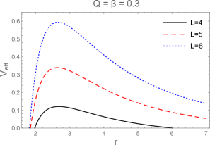
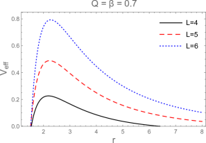
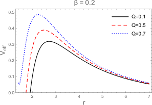
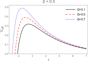
Figure 4: In the upper panel, effective potential is plotted as a function of $r$ for different values of angular momentum with a fixed spin parameter $a=0.5$. In the lower panel, $V_{\mathrm{eff}}$ is plotted as a function of $r$ for different values of charge parameter with the corresponding fixed parameters, spin $a=0.5$ and angular momentum $L=0.5$.

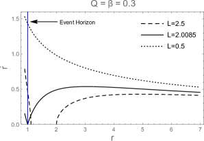
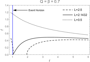
Figure 5: The variation of $\dot{r}$ with respect to the radial coordinate for an extremal black hole. In the left panel $Q=\beta=0.3$ and $a_{E}=0.954915061906$ and in the right panel $Q=\beta=0.7$ and $a_{E}=0.72132723117$.

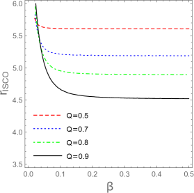
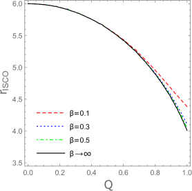
Figure 6: The inner most stable circular orbits by varying the Born-Infeld parameter $\beta$ and charge $Q$ for a static non-rotating EBI black hole.

$$P_{t} =g_{tt}\dot{t}+g_{t\phi}\dot{\phi},$$ (10)

$$P_{\phi} =g_{\phi\phi}\dot{\phi}+g_{t\phi}\dot{t},$$ (11)

where $P_{t}$ and $P_{\phi}$ are the constants of motion. Basically, the two quantities $P_{t}$ and $P_{\phi}$ correspond to the particle’s energy $E$ and the angular momentum $L$, respectively, acting along the axis of symmetry. The overdot denotes differentiation with respect to the proper time $\tau$. The equations of motion of a massive particle are calculated from (10,11) along with the normalization condition $u_{\mu}u^{\mu}=-m_{0}^{2}$, given as below

$$\dot{t} =\frac{1}{r^{2}}\bigg{[}\frac{(a^{2}+r^{2})}{\Delta}\big{(}E(a^{2}+r^{2})-aL\big{)}$$

$$+a\bigg{(}L-aE\bigg{)}\bigg{]},$$ (12)

$$\dot{\phi} =\frac{1}{r^{2}}\bigg{[}\frac{a}{\Delta}\big{(}E(a^{2}+r^{2})-aL\big{)}+\bigg{(}L-aE\bigg{)}\bigg{]},$$ (13)

$$\dot{r} =\pm\frac{\sqrt{\big{(}aL-(a^{2}+r^{2})E\big{)}^{2}-\Delta\big{(}m_{0}^{2}r^{2}+(L-aE)^{2}\big{)}}}{r^{2}}.$$ (14)

The $+$ and $-$ signs of  (14) refer respectively, to the outgoing and incoming geodesics. In order to understand the motion of the test particle in the vicinity of EBI gravity thoroughly we must evaluate the effective potential, which is straightforwardly worked out using  (14).

$$\frac{1}{2}\dot{r}^{2} +V_{\mathrm{eff}}=0,$$ (15)

$$V_{\mathrm{eff}} =-\frac{\big{(}aL-(a^{2}+r^{2})E\big{)}^{2}-\Delta\big{(}m_{0}^{2}r^{2}+(L-aE)^{2}\big{)}}{2r^{4}}.$$ (16)

When an accelerated particle reaches the black hole, it can most probably continue its motion in the spacetime gravity. In Fig. (4) the effective potential is shown by varying the angular momentum of the incoming test particle for a fixed $Q=\beta$. It is viewed that the potential barrier rises for the larger values of $L$ interpreting that a boosted particle can quickly start circling the black hole. Also, the feasibility of a particle’s motion in the black hole surroundings is increased if the electric field intensity attains its maximum strength.
The magnitude of a particle’s momentum plays a vital role to perceive its geodesics in the gravitational space-time. Thus one may get the critical value of the angular momentum from (12) when $r\rightarrow r^{E}_{H}$, i.e, $L_{c}=\frac{(a^{2}+(r^{E}_{H})^{2})E}{a}$. Fig. (5) gives a comprehensible demonstration of the geodesics in EBI space-time. The particle with $L<L_{c}$ is always captured by the black hole gravity and falls exactly at the horizon if $L=L_{c}$, however, when $L>L_{c}$ the geodesics never fall into the black hole.
The solution to the simultaneous equations $\partial_{r}V_{\mathrm{eff}}=\partial^{2}_{r}V_{\mathrm{eff}}=0$ defines the innermost stable circular orbit $r_{\mathrm{ISCO}}$ of the particle Shay:2014a ; Zasl:2015a ; Vrba:2020a ; Babar:2016a ; Babar:2017a ; Shay:2020a ; Shay:2020b . Fig. (6) illustrates the $r_{\mathrm{ISCO}}$ for a static non-rotating EBI gravity by varying the Born-Infeld parameter and charge $Q$ of the black hole. It is observed that the radius of the orbits becomes smaller as $\beta$ and $Q$ increases, however the decrease is seen to be relatively higher in case of the black hole’s charge. More precisely we can say that the charge of the EBI black hole besides its infinite gravity significantly enhances its ability to grasp the incoming particle in its vicinity and by increasing the amount of charge the ISCO as a result comes closer to the black hole. This behaviour is reminiscent of what has been investigated for the Kerr-Newman spacetime in Liu:2017a .

III.1 Near Horizon collision

Now we analyse the ultrahigh energy produced as a result of a two-particle collision near the horizon of EBI black hole. We consider particles with the same mass $m_{0}$ and different four-velocities $\mathrm{u_{1}}$ and $\mathrm{u_{2}}$. The CM energy $E_{\mathrm{c.m}}$ of collision between two particles at the radial coordinate $r$ is given by the following expression Bds:2009a ,

$$E_{\mathrm{c.m}}=m_{0}\sqrt{2}\sqrt{1-g_{\mu\nu}\mathrm{u_{1}}^{\mu}\mathrm{u_{2}}^{\nu}}.$$ (17)

By substituting (12-14) in the above mentioned energy frame we get

$$\frac{E_{\mathrm{c.m}}^{2}}{2m{{}_{0}}^{2}} =-\frac{\mathcal{K}}{r^{2}\Delta},$$ (18)

where $\mathcal{K}$ is given as below,

$$\mathcal{K} =-2r^{4}+2r^{3}-r^{2}\big{(}2a^{2}+Q^{2}(r)-L_{1}L_{2}\big{)}$$

$$-2a^{2}r+2r\big{[}a(L_{1}+L_{2})-L_{1}L_{2}\big{]}$$

$$+Q^{2}(r)\big{(}a-L_{1}\big{)}\big{(}a-L_{2}\big{)}$$

$$+\sqrt{\big{(}a^{2}+r^{2}-aL_{1}\big{)}^{2}-\Delta\big{[}r^{2}+(a-L_{1})^{2}\big{]}}$$

$$\times\sqrt{\big{(}a^{2}+r^{2}-aL_{2}\big{)}^{2}-\Delta\big{[}r^{2}+(a-L_{2})^{2}\big{]}}.$$ (19)

Q	$\beta$	$Q(r)_{E}$	$a_{E}$	$r^{E}_{H}$	$L_{1}$	$L_{2}$
0	0	0	1	1	-4.82843	2
0.2	0.2	0.19792	0.98021707	1.00141	-4.80013	2.00327
0.3	0.3	0.296864	0.95491506	1.00304	-4.76386	2.0085
0.4	0.4	0.39579	0.91832659	1.00512	-4.71127	2.01845
0.5	0.5	0.494701	0.86903103	1.00751	-4.64012	2.03709
0.6	0.6	0.593595	0.80470045	1.01008	-4.54673	2.07259
0.7	0.7	0.692477	0.72132723	1.01274	-4.42477	2.1432

Table 3: The limiting values of the angular momentum for different extremal cases of a rotating EBI black hole.

Q	$\beta$	$a$	$r^{-}_{H}$	$r^{+}_{H}$	$L_{1}$	$L_{2}$
0.2	0.2	0.9	0.663948	1.38792	-4.74224	2.56572
0.3	0.3	0.8	0.632149	1.52037	-4.64939	2.78645
0.4	0.4	0.7	0.638054	1.59260	-4.54509	2.93519
0.5	0.5	0.6	0.653747	1.62586	-4.42765	3.04241
0.6	0.6	0.5	0.674623	1.62645	-4.29465	3.11902
0.7	0.7	0.3	0.686800	1.65050	-4.04668	3.33159

Table 4: The limiting values of the angular momentum for different non-extremal cases of a rotating EBI black hole.

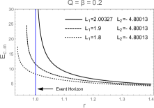
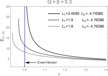
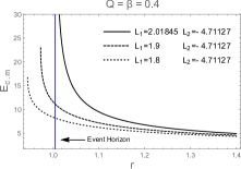
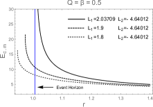
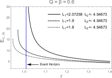
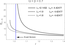
Figure 7: The center-of-mass energy $E_{\mathrm{c.m}}$ dependence of the radial coordinate $r$ for an extremal black hole for various $Q=\beta$ values.

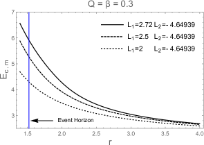
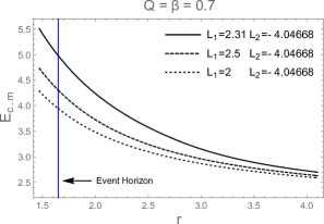
Figure 8: The center-of-mass energy $E_{\mathrm{c.m}}$ dependence of the radial coordinate $r$ for a non-extremal black hole. In the left panel $a=0.8$ and in the right panel $a=0.3$.

In our discussion, the participating particles have the same intrinsic identities and are mainly distinguished by their angular momenta $L_{1}$ and $L_{2}$. Here, for the sake of simplicity, we shall take the conserved energies $E_{1}/m_{0}$=$E_{2}/m_{0}$=1. It is worth mentioning that an arbitrarily high amount of energy is obtained when the test particle approaching the back hole has the critical angular momentum $L_{c}$ Josh:2015a ; Josh:2016a . The limiting values of the angular momentum along with the corresponding spin parameters and the horizons for the extremal and non-extremal EBI space-time are presented, respectively, in the Tables (3,4). The $E_{\mathrm{c.m}}$ generated as a result of collision near the horizon of an extremal black hole for different values of $Q=\beta$ is shown in Fig. (7). Quite similar to a charged Kerr-Newman gravity Wei:2011a , the CM energy instantaneously diverges near the EBI horizon whenever the incoming particle is equipped with the critical parameters of the motion, on the other hand, the particles admitting $L<L_{c}$ contribute only a finite $E_{\mathrm{c.m}}$. Nonetheless, if we consider a collision in a non-extremal space-time background, we attain a limited $E_{\mathrm{c.m}}$ irrespective of the event’s location, see Fig. (8).

IV Strong-field lensing

In this section we shall focus on the strong deflection limit of EBI black hole in the equatorial plane ($\theta=\pi/2$), i.e., both the observer and the source are limited to the equatorial plane. Also, to proceed further we introduce the following dimensionless variables

$$x\to\frac{r}{2M} ,~{}~{}t\to\frac{t}{2M},~{}~{}a\to\frac{a}{2M},~{}~{}q\to\frac{Q}{2M},$$

$$~{}~{}\beta\to\frac{\beta}{2M},$$ (20)

The metric (II) accordingly reduces to the form

$$ds^{2}=-A(x)dt^{2}+B(x)dx^{2}+C(x)d\phi^{2}-2D(x)dtd\phi,$$ (21)

where

$$A(x) = \frac{\Delta-a^{2}}{x^{2}},$$ (22)

$$B(x) = \frac{x^{2}}{\Delta},$$ (23)

$$C(x) = x^{2}+a^{2}\left(2-\frac{\Delta-a^{2}}{x^{2}}\right),$$ (24)

$$D(x) = a\left(1-\frac{\Delta-a^{2}}{x^{2}}\right),$$ (25)

and $\Delta=x^{2}+a^{2}-x+q^{2}(x)$.

$$q^{2}(x) \approx\frac{2\beta^{2}x^{4}}{3}\bigg{(}1-\sqrt{1+\xi^{2}(x)}\bigg{)}$$ (26)

$$+\frac{4q^{2}}{3}\bigg{(}1-\frac{1}{10}\xi^{2}(x)+\frac{1}{24}\xi^{4}(x)\bigg{)}.$$

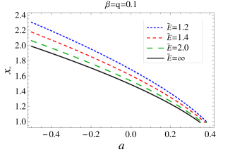
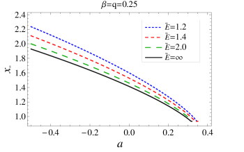
Figure 9: Plot showing the variation of photon sphere radius $x_{m}$ with black hole spin parameter $a$ in different plasma medium. $\tilde{E}=\infty$ corresponds to vacuum.

We assume that the spacetime is filled with a non-magnetized cold plasma whose electron plasma frequency depends on the radius coordinate. We consider the medium to be homogenous but dispersive such that refractive index is constant in space but depends on the wave frequency. The gravitational deflection angle, in this case, is different from the vacuum and depends on the photon frequency. Synge developed the general relativistic geometrical optics in a curved spacetime in a dispersive medium with the reflective index’s angular isotropy. In the subsequent analysis we shall take into consideration a static homogeneous plasma in the gravitational field with a refractive index $n$ obtained by Synge Synge:1960b

$$n^{2}=1+\frac{p_{\alpha}p^{\alpha}}{(p_{\beta}u^{\beta})^{2}},$$ (27)

$p_{\alpha}$ and $u^{\beta}$ indicate the four-momentum and four-velocity of the massless particle. One may retrieve the vacuum case when $n=1$. We define a specific form of the refractive index $n$ for a precise analysis Bin:2010a ; Tsp:2011a

$$n^{2}=1-\frac{{\omega^{2}_{e}}}{[\omega(x^{i})]^{2}}.$$ (28)

Here, $\omega_{e}$ is the plasma electron frequency and $\omega(x^{i})$ is the photon frequency depending on the spatial coordinates $x^{i}$ detected by a distant observer. The light can propagate through the plasma medium if and only if the inequality, $\omega^{2}>{\omega^{2}_{e}}$ is satisfied. The plasma frequency admits the following analytic expression

$$\omega^{2}_{e} =\frac{4\pi e^{2}N(x^{i})}{m}=K_{e}N(x^{i}),$$ (29)

where $e$, $m$ and $N(x^{i})$ are the charge, mass and number density of the electron, respectively Rog:2015a . The Hamiltonian for the photon around the EBI black hole surrounded by plasma has the following form

$$H(x^{i},p_{i})=\frac{1}{2}\left(g^{ik}p_{i}p_{k}+\omega_{e}^{2}\right)=0,$$ (30)

where $g^{ij}$ is the contravariant metric tensor. Using Eq.(30), the Hamiltonian differential equations which are given by

$$\frac{dx^{i}}{d\lambda}=\frac{\partial H}{\partial p_{i}},~{}~{}~{}~{}~{}~{}\frac{dp_{i}}{d\lambda}=-\frac{\partial H}{\partial x^{i}},$$ (31)

give two constants of motion which are Energy $E$ and angular momentum $L$ of the photon. The conserved quantities $E$ and $L$, attain the form

$$E=-p_{t}=\omega~{}~{}~{}~{}~{}~{}~{}L=p_{\phi}.$$ (32)

We introduce notation $\tilde{L}$ and $\tilde{E}$, by considering a homogeneous plasma with $\omega_{e}=constant$, as

$$\tilde{E}=\frac{-p_{t}}{\omega_{e}}=\frac{\omega}{\omega_{e}}~{}~{}~{}~{}~{}\tilde{L}=\frac{p_{\phi}}{\omega_{e}}.$$ (33)

The first order geodesic equation in the equatorial plane in terms of $\tilde{E}$ and $\tilde{L}$ reduce to the following form

$$\dot{t} = \frac{\omega_{e}\left(\tilde{E}C(x)-\tilde{L}D(x)\right)}{A(x)C(x)+D(x)^{2}},$$ (34)

$$= \frac{\omega_{e}}{x^{2}}\bigg{[}\frac{(a^{2}+x^{2})}{\Delta}\big{(}\tilde{E}(a^{2}+x^{2})-a\tilde{L}\big{)}+a\big{(}\tilde{L}-a\tilde{E}\big{)}\bigg{]},$$

$$\dot{\phi} = \frac{\omega_{e}\left(\tilde{E}D(x)+\tilde{L}A(x)\right)}{A(x)C(x)+D(x)^{2}},$$ (35)

$$= \frac{\omega_{e}}{x^{2}}\bigg{[}\frac{a}{\Delta}\big{(}\tilde{E}(a^{2}+x^{2})-a\tilde{L}\big{)}+\big{(}\tilde{L}-a\tilde{E}\big{)}\bigg{]},$$

$$\dot{x}^{2} =\frac{\omega_{e}^{2}}{B(x)\big{(}A(x)C(x)+D(x)^{2}\big{)}}\bigg{(}\tilde{E}^{2}C(x)-2\tilde{L}\tilde{E}D(x)$$

$$-\tilde{L}^{2}A(x)-\big{(}A(x)C(x)+D(x)^{2}\big{)}\bigg{)},$$

$$=\frac{\omega_{e}^{2}}{x^{4}}\bigg{[}\big{(}a\tilde{L}-(a^{2}+x^{2})\tilde{E}\big{)}^{2}-\Delta\big{(}x^{2}+(\tilde{L}-a\tilde{E})^{2}\big{)}\bigg{]}.$$ (36)

With the condition $\dot{x}\Big{|}_{x=x_{0}}=0$, Eq. (IV) can be solved for $\tilde{L}$ to give

$$\tilde{L(x_{0})} = \frac{-\tilde{E}D(x_{0})+\sqrt{A(x_{0})G(x_{0})+\tilde{E}^{2}D(x_{0})^{2}}}{A(x_{0})}$$ (37)

$$G(x_{0}) = \tilde{E}^{2}C(x_{0})-(A(x_{0})C(x_{0})+D(x_{0})^{2}),$$ (38)

which solves to

$$\tilde{L(x_{0})}=\frac{a\tilde{E}(a^{2}+x_{0}^{2}-\Delta)-x_{0}\sqrt{(a^{2}-\Delta+\tilde{E}^{2}x^{2})\Delta}}{a^{2}-\Delta}$$ (39)

The photon traveling close to the black hole encounters a turning points at $\dot{x}=0$, and at radius $x_{0}=x_{m}$, the deflection angle becomes infinitely large. The radius $x_{m}$ is the photon sphere radius and is the largest solution of the equation

$$\left(G^{\prime}(x_{0})A(x_{0})-A^{\prime}(x_{0})G(x_{0})\right)$$

$$+2\tilde{L}\tilde{E}\left(A^{\prime}(x_{0})D(x_{0})-A(x_{0})D^{\prime}(x_{0})\right)$$ (40)

In Fig. (9), we present the variation of photon sphere with the black hole spin parameter in vacuum and in different plasma medium. The presence of the medium can increase the photon sphere radius. In the case of $a>0$ (prograde orbit), the photons tend to come closer to the black hole compared to $a<0$ (retrograde orbit). Especially for the extreme values of $a$ , the photon sphere radius in the plasma medium tends to be same as in the vacuum for prograde orbits.

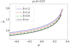
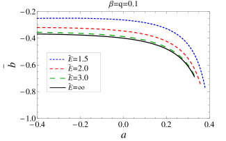
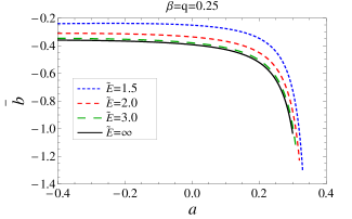
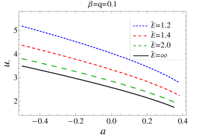
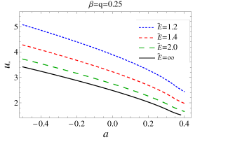
Figure 10: Plot showing the behavior of strong lensing coefficients $\bar{a}$, $\bar{b}$ and $u_{m}$ as a functions of $a$, $q$ for different values of $\tilde{E}$.

Bozza Bozza:2002b ; Bozza:2002af developed the method to find the deflection angle suffered by the light on its way from the source to observer and is given by

$$\alpha_{D}(x_{0})=I_{T}(x_{0})-\pi,$$ (41)

Here, $I_{T}(x_{0})$ is the total azimuthal angle, which on using Eq. (35) and Eq. (IV) takes the form

$$I_{T}(x_{0}) = \frac{\sqrt{B(x)A(x_{0})}(\tilde{E}D(x)+\tilde{L}A(x))}{\sqrt{D(x)^{2}+A(x)C(x}\sqrt{P(x,x_{0})}},$$ (42)

$$P(x,x_{0}) =G(x)A(x_{0})-G(x_{0})A(x)+2\tilde{E}\tilde{L}(A(x)D(x_{0})$$ (43)

$$-A(x_{0})D(x)).$$

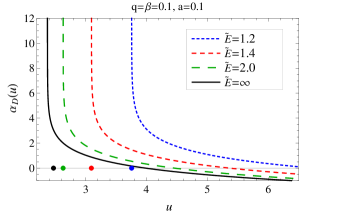
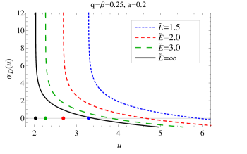
Figure 11: Plot showing the behaviour of deflection angle with the impact parameter for different values of $a$ , $q$ and $\beta$ for different values of $\tilde{E}$. The points on the horizontal line correspond to the impact parameter at which deflection angle diverges.

As the photon approaches the black hole, $x$ decreases from infinity to $x_{0}$ and increases again from $x_{0}$ to infinity as it recedes away. Due to symmetries in space-time, the total change in the azimuthal angle is just twice the change from $x_{0}$ to infinity. If the black hole were not present the total change in the azimuthal angle is $\pi$. Thus deflection angle is accordingly zero. The deflection angle increases as $x_{0}$ approaches $x_{m}$ and diverges logarithmically at $x_{0}=x_{m}$.

Following the method developed by Bozza Bozza:2002b , we can have the deflection angle in SDL as

$$\alpha_{D}(u) = \bar{a}\log\left(\frac{u}{u_{m}}-1\right)+\bar{b}+\mathcal{O}(u-u_{m}).$$ (44)

The details of the calculation can be found in Appendix A. The lensing coefficients $\bar{a}$ and $\bar{b}$ are smaller in vacuum than in the plasma, both decreasing with a just like the Kerr black hole (see Fig. 10). The critical impact parameter, i.e., where the deflection angle diverges, for a fixed values of parameters increases as the frequency of the plasma increases (see Fig. 11).

IV.1 Observables

A geometrical relationship called the lens equation is set up between the observer, the source, and the lens to discuss the strong gravitational lensing by a black hole. In Frittelli ; Frittelli2 ; Perlick there is no requirement for flat background or any condition on the positioning of observer or source, however, to establish a better connection between the models and the observations to get the more clear physical picture we will assume some approximations in the lens equation. The most important and reasonable is the asymptotic approximation i.e., both observer and the source should be in flat spacetime and are not affected by the lens’ curvature effects. It allows us to take all the distance measurements using Euclidean geometry. The asymptotic approximation also considers that the source and observer should be far enough from the lens, and for further implication, the source should lie behind the lens. Even cases of source lying at the back of observer or between observer and lens, which is called retrolensing have been studied

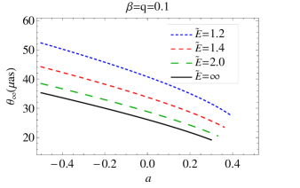
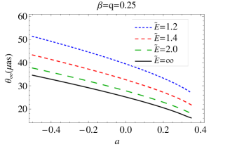
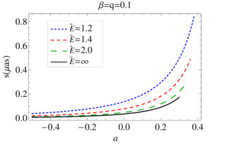
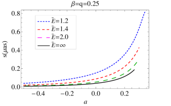
Figure 12: Plot showing the behavior of strong lensing observables as a function of $a$ , for different values of $q$, $\beta$ and $\tilde{E}$ for SgrA*.

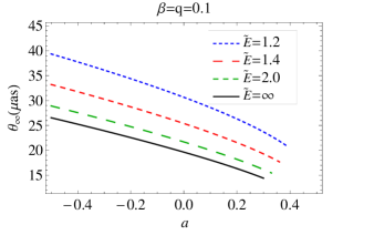
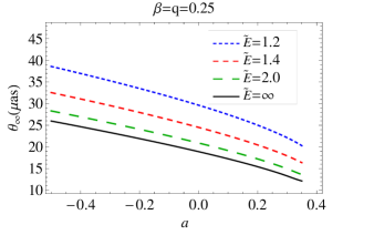
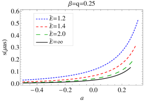
Figure 13: Plot showing the behavior of strong lensing observables as a function of $a$ , for different values of $q$, $\beta$ and $\tilde{E}$ for M87*.

The geometrical configuration for gravitational lensing constitutes a light source $S$, an observer $O$ and a black hole $L$ that acts as a lens and lies between the source and observer. The photons emitted by the source is deviated by the black hole and reach the observer. The observer sees the source’s image at an angle $\theta$ from the optical axis $OL$, whereas, the source is at an angular position of $\beta$ from $OL$. The emission direction and the detection direction make an angle $\alpha_{D}(\theta)$, which is called the deflection angle. The closest approach distance $x_{0}$ is different than the impact parameter $u$ as long as the deflection angle is not vanishing.
Several lens equations, which principally differ from each other for different choices of variables, were introduced however in Bozza:2008ev , the author gave a detailed comparison of varying lens equation and suggested that Ohanian lens is the best approximate lens equation. Using the coordinate independent Ohanian lens equation Oho:1987ev which connects the source and observer positions as

$$\xi = \frac{D_{OL}+D_{LS}}{D_{LS}}\theta-\alpha_{D}(\theta),$$ (45)

$\xi$ is the angle between the lens-source direction and the optical axis. $D_{OL}$ is the observer-lens distance and $D_{LS}$ is the lens-source distance. The angle $\xi$ and $\beta$ are related by

$$\frac{D_{OL}}{\sin(\xi-\beta)} = \frac{D_{LS}}{\sin\beta}.$$ (46)

The lensing effects are most evident when all the objects are almost aligned. It is the case when the relativistic images are most prominent. So we study the case when the angles $\beta$, $\xi$ and $\theta$ are minimal. However, if a ray of light emitted by the source $S$ follow multiple loops around the black hole before reaching the observer, $\alpha$ must be very close to a multiple of 2$\pi$. Replacing $\alpha_{D}(\theta)$ by $\alpha_{D}(\theta)-2n\pi=\Delta\alpha_{n}$, with $n\in N$ and $0<\Delta\alpha_{n}\ll 1$, we can rewrite Eq. (45) for small values of $\beta$, $\xi$ and $\theta$ using Eq. (46) as,

$$\beta = \theta-\frac{D_{LS}}{D_{OL}+D_{LS}}\Delta\alpha_{n}.$$ (47)

Given the angular position of source $\beta$ and the distances of observer and source from the black hole, one can calculate the image positions using Eq. (47). The deflection angle increases as the light ray trajectory get closer to the event horizon, such that for a particular value of $u$, the light form loops around the black hole resulting in $\alpha_{D}(\theta)>2\pi$. With further decreasing impact parameter, the light ray winds several times around the black hole before escaping to the observer. Finally, for critical impact parameter, corresponding to the closest distance $x_{m}$, the deflection angle diverges. For each loop of the light geodesic, there is a particular value of impact parameter at which light reaches the observer from the source. So infinite sequence of images will be formed on each side of the lens. Equation (44) with $\alpha_{D}(\theta_{n}{{}^{0}})=2n\pi$ leads to

$$\theta_{n}{{}^{0}} = \frac{u_{m}}{D_{OL}}(1+e_{n}),$$ (48)

where

$$e_{n} = e^{\frac{q-2n\pi}{p}}.$$ (49)

Here, $n$ is the number of loops followed by the photons around the black hole. The deflection angle is expanded around $\theta_{n}{{}^{0}}$ as:

$$\alpha_{D}(\theta)=\alpha_{D}(\theta_{n}{{}^{0}})+\frac{\partial\alpha_{D}(\theta)}{\partial\theta}\Bigg{|}_{\theta_{n}{{}^{0}}}(\theta-\theta_{n}{{}^{0}})+\mathcal{O}(\theta-\theta_{n}{{}^{0}}).$$ (50)

On using (48) and setting $\Delta\theta_{n}=(\theta-\theta_{n}{{}^{0}})$ we obtain

$$\Delta\alpha_{n} = -\frac{\bar{a}D_{OL}}{u_{m}e_{n}}\Delta\theta_{n}.$$ (51)

Finally the lens equation (47) becomes

$$\beta = (\theta_{n}{{}^{0}}+\Delta\theta_{n})+\frac{D_{LS}}{D_{OL}+D_{LS}}\Bigg{(}\frac{\bar{a}D_{OL}}{u_{m}e_{n}}\Delta\theta_{n}\Bigg{)}.$$ (52)

The second term in the above equation is very small as compared to the third term, there by neglecting it, we get

$$\theta_{n} = \theta_{n}{{}^{0}}+\frac{D_{OL}+D_{LS}}{D_{LS}}\left(\frac{u_{m}e_{n}}{\bar{a}D_{OL}}(\beta-\theta_{n}{{}^{0}})\right).$$ (53)

The above equation, for $\beta>0$, determines images only on the same side of the source ($\theta>0$). To obtain the images on the opposite side, one can solve the same equation with the source placed at $-\beta$. Finally using Eq. (53), we obtain full set of primary ($+\beta$) and secondary images ($-\beta$).

If the outermost image can be separated from the inner packed one, we can have following observables as

$$\theta_{\infty} = \frac{u_{m}}{D_{OL}},$$ (54)

$$s = \theta_{1}-\theta_{\infty}\approx\theta_{\infty}(e^{\frac{\bar{b}-2\pi}{\bar{a}}}),$$ (55)

Table 5: Estimates for lensing observables and strong lensing coefficients for the black hole Sgr A* and M87 for different values of $a$, $q$ and $\tilde{E}$. $R_{s}=2GM/c^{2}$ is the Schwarzschild radius.

				Sgr A*		M87*		Lensing Coefficients
$a$	$q$	$\beta$	$\tilde{E}$	$\theta_{\infty}$ ($\mu$as)	$s$ ($\mu$as)	$\theta_{\infty}$ ($\mu$as)	$s$ ($\mu$as)	$\bar{a}$	$\bar{b}$	$u_{m}/R_{s}$
0.0	0.0	0.0	$\infty$	26.3299	0.0329518	19.782	0.0247572	1.0000	-0.40023	2.59808
0.0	0.10	0.10	1.2	40.8014	0.136406	30.6547	0.102484	1.14818	-0.262399	4.02604
	0.10	0.10	1.4	33.8068	0.0768462	25.3996	0.0577357	1.08896	-0.344909	3.33586
	0.10	0.10	2.0	28.8801	0.0465492	21.6981	0.0349731	1.0372	-0.386451	2.84972
	0.10	0.10	$\infty$	26.1546	0.033707	19.6504	0.0253245	1.0042	-0.398845	2.58079
0.0	0.25	0.25	1.2	39.4685	0.151685	29.6533	0.113963	1.17496	-0.251322	3.89452
	0.25	0.25	1.4	32.6493	0.0864492	24.5299	0.0649506	1.11551	-0.336246	3.22164
	0.25	0.25	2.0	27.8451	0.052903	20.9204	0.0397468	1.06329	-0.379309	2.74759
	0.25	0.25	$\infty$	25.1872	0.0385673	18.9235	0.0289762	1.02991	-0.392364	2.48532
0.1	0.10	0.10	1.2	38.0561	0.194843	28.5922	0.146388	1.24476	-0.282442	3.75516
	0.10	0.10	1.4	31.3725	0.114023	23.5706	0.0856672	1.18444	-0.37017	3.09565
	0.10	0.10	2.0	26.6578	0.0715111	20.0284	0.0537274	1.13104	-0.413689	2.63043
	0.10	0.10	$\infty$	24.0469	0.0530149	18.0668	0.0398309	1.09672	-0.425657	2.37281
0.1	0.25	0.25	1.2	36.58	0.222988	27.4831	0.113963	1.28608	-0.276002	3.6095
	0.25	0.25	1.4	30.0954	0.132432	22.6111	0.0994979	1.22571	-0.367598	2.96964
	0.25	0.25	2.0	25.5194	0.0841841	19.1731	0.0632488	1.17203	-0.414005	2.5181
	0.25	0.25	$\infty$	22.9847	0.062994	17.2688	0.0473283	1.1375	-0.427547	2.268
0.3	0.10	0.10	1.2	31.565	0.494733	23.7153	0.3717	1.61897	-0.444896	3.11465
	0.10	0.10	1.4	25.6834	0.318908	19.2963	0.239601	1.55668	-0.548617	2.53428
	0.10	0.10	2.0	21.5156	0.218539	16.165	0.164192	1.49933	-0.598094	2.12304
	0.10	0.10	$\infty$	19.1999	0.172071	14.4252	0.129279	1.4616	-0.6079	1.89454
0.3	0.25	0.25	1.2	29.4773	0.638265	22.1467	0.479538	1.82734	-0.720304	2.90865
	0.25	0.25	1.4	23.8921	0.428647	17.9505	0.322049	1.77993	-0.873316	2.35753
	0.25	0.25	2.0	19.9254	0.307738	14.9703	0.231208	1.74127	-0.978784	1.96612
	0.25	0.25	$\infty$	17.7162	0.251906	13.3104	0.189261	1.72008	-1.03261	1.74813

Here, $\theta_{\infty}$ is the angular position acquired by the set of images in the limit $n\to\infty$ or in other words angular radius of photon sphere. s is the angular seperation between outermost image ($n=1$) and innermost packed images ($n=2,3,4...\infty$).

The EHT using VLBI technique, released the first image of supermassive black hole M87* in the center of nearby elliptical galaxy. The image (shadow) is an asymmetric emission ring with diameter of $42\pm 3\mu$as and indicated mass of the black hole $(6.5\pm 0.7)\times 10^{9}M_{\odot}$. This offers a new tool to test black hole in the strong field regime. Motivated by this we consider the supermassive black holes Sgr A* in our galactic center and M87* in nearby galaxy Messier 87 as lens for numerical estimation of observables. The masses and distances from earth according to the latest observational data for Sgr A* Do:2019vob are $M=4.3\times 10^{6}M_{\odot}$, $D_{OL}=8.35$ Kpc and for M87* Akiyama:2019vo are $M=(6.5\pm 0.7)\times 10^{9}M_{\odot}$, $D_{OL}=(16.8\pm 0.8)$ Mpc respectively. We have tabulated the strong lensing coefficients $\bar{a}$, $\bar{b}$, $u_{m}$ and the observables angular position of innermost image $\theta_{\infty}$ and separation between the first image and the inner packed ones $s$ in Table 5. For comparisons, we have estimated these values for the Schwarzschild black hole and Kerr-Newman black hole and found that the angular position and angular separation for EBI black hole are larger. In Table 6, we have calculated the deviation of the coefficients and observables of the EBI black hole from the Kerr black hole for fixed value of spin parameter ($a=0.3$) and found that in case of EBI black hole the images are formed closer to the optical axis but are more packed than the Kerr black hole. The deviation of angular positions can reach a maximum value of $2.5\mu$as for Sgr A* and $1.8\mu$as for M87*, which with the current observational facilities is impossible to resolve. From the plots in Figs. (12) and  (13) it can be immediately followed that angular separation $s$ increases but angular position ($\theta_{\infty}$) decreases with spin parameter $a$. It is worth noting that both angular separation and angular position increase in the presence of plasma than in vacuum. Also, for fixed values of $a$ and $\tilde{E}$, both angular position and angular separation decreases with charge $q$.

Table 6: Deviation of the lensing observables of EBI black holes from Kerr black hole by taking Sgr A* and M87* as lens, where $\delta X=X_{\text{Kerr}}-X_{\text{EBI}}$

				Sgr A*		M87*		Lensing Coefficients
$a$	$q$	$\beta$	$\tilde{E}$	$\delta\theta_{\infty}$ ($\mu$as)	$\delta s$ ($\mu$as)	$\delta\theta_{\infty}$ ($\mu$as)	$\delta s$ ($\mu$as)	$\delta\bar{a}$	$\delta\bar{b}$	$\delta u_{m}/R_{s}$
0.3	0.25	0.25	1.2	2.4438	-0.163407	1.83607	-0.12277	-0.231673	0.288928	0.24114
	0.25	0.25	1.4	2.09623	-0.124046	1.57493	-0.0931977	-0.247045	0.340692	0.206844
	0.25	0.25	2.0	1.85985	-0.100026	1.39733	-0.075151	-0.266229	0.398848	0.183519
	0.25	0.25	$\infty$	1.73419	-0.088959	1.30292	-0.0668363	-0.283155	0.444148	0.17112

V Weak-field lensing

In this section we review the effects of gravitational lensing in the background of EBI black hole surrounded by a plasma considering a weak-field approximation defined as follows,

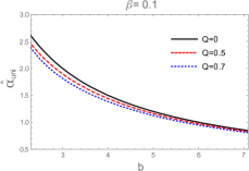
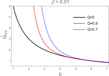
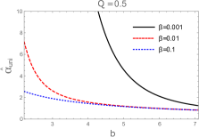
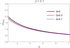
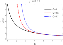
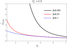
Figure 14: Deflection angle $\hat{\alpha}_{b}$ as a function of the impact parameter $b$ for different charge $Q$ and Born-Infeld $\beta$ values for fixed $\frac{\omega^{2}_{e}}{\omega^{2}}=0.5$(upper panel). Deflection angle $\hat{\alpha}_{SIS}$ as a function of the impact parameter $b$ for different charge $Q$ and Born-Infeld $\beta$ values for fixed $\frac{\omega^{2}_{c}}{\omega^{2}}=0.5$ (lower panel).

$$g_{\alpha\beta}=\eta_{\alpha\beta}+h_{\alpha\beta},$$ (56)

where $\eta_{\alpha\beta}$ and $h_{\alpha\beta}$ specify the Minkowski metric and perturbation metric, respectively.

$$\eta_{\alpha\beta} ={\rm diag}(-1,1,1,1)\ ,$$

$$h_{\alpha\beta} \ll 1,\quad h_{\alpha\beta}\rightarrow 0\quad{\rm under}\quad x^{\alpha}\rightarrow\infty\ ,$$

$$g^{\alpha\beta} =\eta^{\alpha\beta}-h^{\alpha\beta},\ \ \ h^{\alpha\beta}=h_{\alpha\beta}\ .$$ (57)

We follow the notion in Abu:2017aa by taking into account the weak-field approximation and weak plasma strength for the photon propagation along $z$ axis to get the angle of deflection,

$$\hat{\alpha}_{i} =\frac{1}{2}\int_{-\infty}^{\infty}\bigg{(}h_{33_{,}i}+\frac{\omega^{2}}{\omega^{2}-\omega^{2}_{e}}h_{00_{,}i}-\frac{K_{e}}{\omega^{2}-\omega^{2}_{e}}N{{}_{,}i}\bigg{)}dz.$$ (58)

Note that, the $\hat{\alpha}_{i}<0$ and $\hat{\alpha}_{i}>0$ indicate the deflection towards and away from the central object, respectively. In the last expression the values of $\omega_{e}$ and $n$ are set to limitations at infinity and $\omega(\infty)=\omega$. At large $r$, the black hole metric could be approximated to Bin:2010a .

$$ds^{2}=ds^{2}_{0}+\left(\frac{2M}{r}-\frac{Q^{2}(r)}{r^{2}}\right)dt^{2}+\left(\frac{2M}{r}-\frac{Q^{2}(r)}{r^{2}}\right)dr^{2},$$ (59)

where $ds^{2}_{0}=-dt^{2}+dr^{2}+r^{2}(d\theta^{2}+\sin^{2}\theta d\phi^{2})$. In the Cartesian coordinates the components $h_{\alpha\beta}$ can be written as

$$h_{00}= \left(\frac{R_{g}}{r}-\frac{Q^{2}(r)}{r^{2}}\right),$$

$$h_{ik}= \left(\frac{R_{g}}{r}-\frac{Q^{2}(r)}{r^{2}}\right)n_{i}n_{k}\ ,$$

$$h_{33}= \left(\frac{R_{g}}{r}-\frac{Q^{2}(r)}{r^{2}}\right)\cos^{2}x,$$ (60)

where $R_{g}=2M$, $\cos x=z/\sqrt{b^{2}+z^{2}}$ and $r=\sqrt{b^{2}+z^{2}}$. We apply the approximation $\beta\rightarrow\infty$ to the series expansion of $Q^{2}(r)$ (9),

$$Q^{2}(r)=Q^{2}-\frac{2Q^{4}}{15r^{4}\beta^{2}}.$$ (61)

Using the above mentioned expressions in the formula (58) one can compute the light deflection angle for a black hole in plasma in terms of the impact parameter $b$, given as below

$$\hat{\alpha}_{b} =\bigintssss_{-\infty}^{\infty}\frac{b}{2r}\Bigg{(}\partial_{r}\bigg{(}\bigg{(}\frac{R_{g}}{r}-\frac{Q^{2}(r)}{r^{2}}\bigg{)}\cos^{2}x\bigg{)}$$

$$+\partial_{r}\bigg{(}\frac{R_{g}}{r}-\frac{Q^{2}(r)}{r^{2}}\bigg{)}\frac{\omega^{2}}{\omega^{2}-\omega^{2}_{e}}-\frac{K_{e}}{\omega^{2}-\omega^{2}_{e}}\partial_{r}N\Bigg{)}dz,$$ (62)

V.1 Uniform Plasma

Now, we discuss the light deflection in the presence of a uniform plasma, thereby considering $\omega_{e}$ as a constant quantity and taking in the approximation $1-n<<\frac{\omega_{e}}{\omega}$. As a result $\partial_{r}N$ vanishes and the angle of deflection takes the form

$$\hat{\alpha}_{\mathrm{uni}} =-\bigg{(}\frac{\omega^{2}}{\omega^{2}-\omega^{2}_{e}}\bigg{)}\bigg{(}\frac{\pi Q^{2}}{2b^{2}}-\frac{\pi Q^{4}}{8b^{6}\beta^{2}}-\frac{R_{g}}{b}\bigg{)}$$

$$-\bigg{(}\frac{\pi Q^{2}}{4b^{2}}-\frac{\pi Q^{4}}{48b^{6}\beta^{2}}-\frac{R_{g}}{b}\bigg{)}.$$ (63)

The upper panel of Fig. (14) illustrates the angle of deflection as a function of the impact parameter. On varying the charge for a fixed $\beta$, the angle of deflection executes two opposite behaviours depending on the value of $\beta$. The deviation of photons is larger as the value of $Q$ decreases when allotted with a comparatively larger $\beta$, hence, $\hat{\alpha}_{\mathrm{uni}}$ is maximum for $Q=0$, which basically refers to the Schwarzschild gravity. It is noticed that by increasing $\beta$ for a fixed charge $Q$ the results are consistent, and the angle of deflection reduces in any case.

V.2 Singular isothermal sphere

We shall now examine the photon deflection by the black hole surrounded by a singular isothermal sphere, which was modeled in Chnd:1939a ; Jbin:1987a and has up till now played an important part to explore the len’s property of the galaxies and clusters. The density distribution has the form

$$\rho(r)=\frac{\sigma^{2}_{v}}{2\pi r^{2}},$$ (64)

where $\sigma^{2}_{v}$ is a one-dimensional velocity dispersion. The concentration of the plasma has the form

$$N(r)=\frac{\rho(r)}{\kappa m_{p}},$$ (65)

where $m_{p}$ is the proton mass and $\kappa$ is a non-dimensional coefficient which is related to the dark matter contribution. Utilizing (29,64,65) the plasma frequency takes the form

$$\omega^{2}_{e}=K_{e}N(r)=\frac{K_{e}\sigma^{2}_{v}}{2\pi\kappa m_{p}r^{2}}.$$ (66)

The angle of deflection using the latter particulars can be conveniently computed as below Bin:2010a ,

$$\hat{\alpha}_{\mathrm{SIS}} =\frac{\omega^{2}_{c}R^{2}_{g}}{\omega^{2}b^{2}}\bigg{(}\frac{1}{2}-\frac{3Q^{2}}{8b^{2}}+\frac{7Q^{4}}{64b^{6}\beta^{2}}+\frac{2R{{}_{g}}}{3b\pi}\bigg{)}-$$

$$\bigg{(}\frac{3\pi Q^{2}}{4b^{2}}-\frac{7\pi Q^{4}}{48b^{6}\beta^{2}}-\frac{2R_{g}}{b}\bigg{)},$$ (67)

we get $\omega^{2}_{c}$ which is another plasma constant and has the following analytic expression.

$$\omega^{2}_{c}=\frac{\sigma^{2}_{v}K_{e}}{2\kappa m_{p}R^{2}_{g}}.$$ (68)

The lower panel of Fig. (14) shows the angle of deflection $\hat{\alpha}_{\mathrm{SIS}}$ as a function of the impact parameter considering a black hole veiled by a singular isothermal sphere. The results obtained for distinct $Q$ and $\beta$ values, altogether share a common thread with the uniform plasma case, but, however the angle of deflection is relatively smaller as by the black hole surrounded with a uniform plasma, i.e, $\hat{\alpha}_{\mathrm{uni}}>\hat{\alpha}_{\mathrm{SIS}}$, see details in Babar:2021a .

VI Conclusion

In this paper we constructed an insightful discussion regarding the rotating black hole’s structure, centre-of-mass energy and gravitational lensing in Einstein-Born-Infeld gravity. It is searched out that the radii of the event horizons, the static limit surfaces and ISCOs experience a uniform decrease as the strength of black hole’s charge intensifies but the Cauchy horizon on the contrary, exhibits an increase. Furthermore, our investigation ensures the BSW effect in the EBI space-time, henceforth the centre-of-mass energy diverges near the horizon just like the other charged rotating black holes, in our case we specifically considered the Kerr-Newman black hole.

The gravitational lensed photons considering a uniform plasma and a singular isothermal sphere are also part of the context. Unfortunately due to extinction of radiation in the vicinity of galactic center, the observation of relativistic images is an uphill task. In addition, the radiation from the accreting materials badly influences the observation of these images. Compared to the weak lensing, these obstacles are even bigger for the strong lensing. For relativistic images to be more prominent, the lens components (the source, the observer and the lens) should be highly aligned. A suitable source for the strong lensing could be a supernova but the probability of it to be aligned with the lens and observer is extremely small. Despite this, there is no doubt that observation of relativistic images would be one of the most important discovery in the field of astronomy and would have immense implication for general relativity and relativistic physics, one of which is that it could provide a test for general relativity in the strong field regime.

In this paper it is interpreted that the photons deviate at a larger angle when a uniform plasma walls in the black hole. The light deflection coefficients $\bar{a}$ and $\bar{b}$, in the strong field limits, and their variance with the rotational parameter $a$ for different plasma frequency as well as in vacuum are calculated. The effect of plasma result in the increase of the photon sphere radius, the deflection angle and the strong deflection coefficients $\bar{a}$ and $\bar{b}$ as compared to the Kerr-Newman black hole. The lensing observables angular positions and the angular separation between the relativistic images show similar behavior. It is also shown in the paper that with increasing spin the impact of plasma on strong gravitational lensing becomes smaller as the spin parameter increases in the prograde orbit ($a>0$) especially for the case of an extreme black hole, the strong gravitational effects in the homogenous plasma are same as the case in vacuum for $a>0$. Also, in our analysis, the EBI gravity has sustained the regularity of a charged black hole effectively in all aspects. In reality, the plasma can be significantly non-uniform in the close vicinity of compact objects like black holes. Such cases, though complicated, will be considered in our later research.

VII Appendix A: Calculting deflection angle in Strong Deflection Limit

In this section we describe the details of calculation for the deflection angle in strong deflection limit by EBI black hole using the approach discussed in Bozza:2001aa . The metric for EBI black hole when both observer and source are in equatorial plane is given by

$$ds^{2}=-A(x)dt^{2}+B(x)dx^{2}+C(x)d\phi^{2}-2D(x)dtd\phi,$$ (69)

where

$$A(x) = \frac{\Delta-a^{2}}{x^{2}},$$ (70)

$$B(x) = \frac{x^{2}}{\Delta},$$ (71)

$$C(x) = x^{2}+a^{2}\left(2-\frac{\Delta-a^{2}}{x^{2}}\right),$$ (72)

$$D(x) = a\left(1-\frac{\Delta-a^{2}}{x^{2}}\right),$$ (73)

and $\Delta=x^{2}-2Mx+a^{2}+q^{2}(x)$,

$$q^{2}(x) \approx\frac{2\beta^{\prime 2}x^{4}}{3}\bigg{(}1-\sqrt{1+\xi^{2}(x)}\bigg{)},$$

$$+\frac{4q^{2}}{3}\bigg{(}1-\frac{1}{10}\xi^{2}(x)+\frac{1}{24}\xi^{4}(x)\bigg{)},$$ (74)

Here $x$ is in the unit of Schwarzschild radius. Using Eq.(35), Eq.(IV) we have

$$\frac{d\phi}{dx} = \frac{\sqrt{B(x)A(x_{0})}(\tilde{E}D(x)+\tilde{L}A(x))}{\sqrt{D(x)^{2}+A(x)C(x}\sqrt{P(x,x_{0})}},$$ (75)

$$P(x,x_{0}) =G(x)A(x_{0})-G(x_{0})A(x)+2\tilde{E}\tilde{L}(A(x)D(x_{0})$$ (76)

$$-A(x_{0})D(x)),$$

where $x_{0}$ is the distance of closest approach to the black hole. The deflection angle will be

$$\alpha_{D}(x_{0})=2\int_{x_{0}}^{\infty}\frac{d\phi}{dx}dx-\pi\equiv I_{T}(x_{0})-\pi.$$ (77)

To solve the integral (77), we define a variable

$$z=1-\frac{x_{0}}{x},$$ (78)

such that the integral (77) reduces to

$$I_{T}(x_{0}) = \int_{0}^{1}R(z,x_{0})f(z,x_{0})dz,$$ (79)

with the functions

$$R(z,x_{0}) = \frac{\sqrt{B(x)A(x_{0})}(\tilde{E}D(x)+\tilde{L}A(x))}{\sqrt{D(x)^{2}+A(x)C(x}},$$ (80)

$$f(z,x_{0}) = \frac{1}{\sqrt{A(x_{0})-\frac{A(x)}{C(x)}C(x_{0})}},$$ (81)

where $x=\frac{x_{0}}{1+z}$. Taking Taylor expansion of the expression under the square root in Eq. (81) we have

$$f_{0}(z,x_{0}) = \frac{1}{\sqrt{\zeta(x_{0})z+\eta(x_{0})z^{2}}},$$ (82)

where

$$\zeta(x_{0}) = \frac{x_{0}}{C(x_{0})}\left[C^{\prime}(x_{0})A(x_{0})-A^{\prime}(x_{0})C(x_{0})\right],$$ (83)

$$\eta(x_{0}) = \frac{1}{2C(x_{0})^{2}}\Big{[}2x_{0}C(x_{0})(A(x_{0})C^{\prime}(x_{0})-A^{\prime}(x_{0})C(x_{0}))$$ (84)

$$+ 2x_{0}^{2}(C(x_{0})A^{\prime}(x_{0})C^{\prime}(x_{0})-A(x_{0})C^{\prime}(x_{0})^{2})$$

$$-x_{0}^{2}C(x_{0})(C(x_{0})A^{\prime\prime}(x_{0})-A(x_{0})C^{\prime\prime}(x_{0}))\Big{]}.$$

The radius of photon sphere $x_{m}$ is given by solving $\zeta(x_{0})=0$. In the integral (79) $R(z,x_{0})$ is regular everywhere but as $x_{0}=x_{m}$, $\zeta(x_{0})=0$ and $f(z,x_{0})\approx 1/z$, which diverges as $z\to 0$. Thus we separate the integral (79) into two parts as

$$I(x_{0})=I_{D}(x_{0})+I_{R}(x_{0}),$$ (85)

where

$$I_{D}(x_{0})=\int_{0}^{1}R(0,x_{m})f_{0}(z,x_{0})dz,$$ (86)

is the divergent part and regular part is

$$I_{R}(x_{0}) = \int_{0}^{1}\Big{(}R(z,x_{0})f(z,x_{0})$$ (87)

$$- R(0,x_{m})f_{0}(z,x_{0})\Big{)}dz.$$

For EBI black hole Eq. (86) can be solved analytically to

$$I_{D}(x_{0}) = -\frac{R(0,x_{m})}{\sqrt{\eta(x_{0})}}\log\Big{(}\frac{\sqrt{\zeta(x_{0})+\eta(x_{0})}+\sqrt{\eta(x_{0})}}{\sqrt{\eta(x_{0})}}\Big{)}$$ (88)

$$+O(x_{0}-x_{m}),$$

And regular term can be solved numerically as

$$I_{R}(x_{0})=I_{R}(x_{m})+O(x_{0}-x_{m}).$$ (89)

By expanding the Eq. (83) and Eq. (84) about $x_{m}$, the deflection angle in SDL becomes

$$\alpha_{D}(x_{0})=-a\log\Big{(}\frac{x_{0}}{x_{m}}-1\Big{)}+b+O(x_{0}-x_{m}),$$ (90)

where

$$a = \frac{R(0,x_{m})}{\sqrt{\eta(x_{m})}},$$ (91)

$$b = -\pi+I_{R}(x_{m}).$$ (92)

The impact parameter can be expressed as

$$u=\frac{\tilde{L}(x0)}{\sqrt{\tilde{E}^{2}-1}}.$$ (93)

We can write deflection angle in terms of impact parameter by expanding Eq. (93) around $x_{m}$ as,

$$\alpha_{D}(u) = -\bar{a}\log\Big{(}\frac{u}{u_{m}}-1\Big{)}+\bar{b}+O(u-u_{m}),$$ (94)

where the strong deflection coefficients are

$$\bar{a}=\frac{a}{2},$$ (95)

$$\bar{b}=b+\bar{a}\log\left(\frac{\eta(x_{m})G(x_{m})}{u_{m}\sqrt{\tilde{E^{2}}-1}A(x_{m})(\tilde{E}D(x_{m})+\tilde{L}A(x_{m}))}\right),$$ (96)

$$u_{m}=\frac{-\tilde{E}D(x_{m})+\sqrt{A(x_{m})G(x_{m})+\tilde{E}^{2}D(x_{m})^{2}}}{\sqrt{\tilde{E}^{2}-1}A(x_{m})}.$$ (97)

References

- (1) K. Akiyama et al., ‘First M87 Event Horizon Telescope Results. VI.The Shadow and Mass of the Central Black Hole’, Ap. J. 875 (2019) 44.
- (2) K. Akiyama et al., ‘First M87 Event Horizon Telescope Results. I. The Shadow of the Supermassive Black Hole’, Ap. J. 875 (2019) 17.
- (3) R. Penrose and R. M. Floyd, ‘Extraction of Rotational Energy from a Black Hole’, Nature Physical Science volume. 229 (1971) 177.
- (4) M. Baados, J. Silk, and S. M. West, ‘Kerr Black Holes as Particle Accelerators to Arbitrarily High Energy’, Phys. Rev. D. 103 (2009) 111102.
- (5) O. B. Zaslavskii, ‘Acceleration of particles as a universal property of rotating black holes’, Phys. Rev. D. 82 (2010) 083004.
- (6) A. A. Grib and Y. V. Pavlov, ‘On particle collisions near rotating black holes’, Gravit. Cosmol. 17 (2011) 42.
- (7) O. B. Zaslavskii, ‘Acceleration of particles by black holes as a result of deceleration: Ultimate manifestation of kinematic nature of BSW effect’, Phys. Lett. B. 712 (2012) 161.
- (8) O. B. Zaslavskii, Energy extraction from extremal charged black holes due to the Banados-Silk-West effect, Phys. Rev. D. 86 (2012) 124039.
- (9) O. B. Zaslavskii, Acceleration of particles near the inner black hole horizon, Phys. Rev. D. 85 (2012) 024029.
- (10) A. Tursunov, M. Kološ, A. Abdujabbarov, B. Ahmedov, and Z. Stuchlík, Acceleration of particles in spacetimes of black string, Phys. Rev. D. 88 (2013) 124001.
- (11) S. R. Shaymatov, B. J. Ahmedov, and A. A. Abdujabbarov, Particle acceleration near a rotating black hole in a Randall-Sundrum brane with a cosmological constant, Phys. Rev. D. 88 (2013) 024016.
- (12) O. B. Zaslavskii, Acceleration of particles by acceleration horizons, Phys. Rev. D. 88 (2013) 104016.
- (13) F. Atamurotov, B. Ahmedov, and S. Shaymatov, Formation of black holes through BSW effect and black hole-black hole collisions, Astrophys. Space. Sci. 347 (2013) 277.
- (14) A. Abdujabbarov, F. Atamurotov, N. Dadhich, B. Ahmedov, and Z. Stuchlk, ‘Energetics and optical properties of 6-dimensional rotating black hole in pure Gauss–Bonnet gravity’, Eur. Phys. J. C. 75 (2015) 399.
- (15) S. -W. Wei, Y. -X. Liu, H. Guo, and C. -E. Fu, ‘Charged spinning black holes as particle accelerators’, Phys. Rev. D. 82 (2010) 103005.
- (16) A. Abdujabbarov, B. Ahmedov, and B. Ahmedov, ‘Energy extraction and particle acceleration around a rotating black hole in Hoava-Lifshitz gravity’, Phys. Rev. D. 84 (2011) 044044.
- (17) A. Abdujabbarov, N. Dadhich, B. Ahmedov, and H. Eshkuvatov, ‘Particle acceleration around a five-dimensional Kerr black hole’, Phys. Rev. D. 88 (2013) 084036.
- (18) S. G. Ghosh and M. Amir, ‘Horizon structure of rotating Bardeen black hole and particle acceleration’, Eur. Phys. J. C. 75 (2015) 553.
- (19) M. Amir and S. G. Ghosh, ‘Rotating Hayward’s regular black hole as particle accelerator’, JHEP 07 (2015) 015
- (20) S. G. Ghosh, P. Sheoran and M. Amir, “Rotating Ayón-Beato-García black hole as a particle accelerator,” Phys. Rev. D. 90 (2014) 103006
- (21) S. Zhang, Y. Liu, and X. Zhang, ‘Kerr–de Sitter and Kerr–anti–de Sitter black holes as accelerators for spinning particles’, Phys. Rev. D. 99 (2019) 064022.
- (22) T. Harada and M. Kimura, ‘Collision of an innermost stable circular orbit particle around a Kerr black hole’, Phys. Rev. D, 83 (2011) 024002.
- (23) M. Patil and P. S. Joshi, ‘Acceleration of particles by Janis-Newman-Winicour singularities’, Phys. Rev. D. 85 (2012) 104014.
- (24) M. Patil and P. S. Joshi, ‘Ultrahigh energy particle collisions in a regular spacetime without black holes or naked singularities’, Phys. Rev. D. 86 (2012) 044040.
- (25) Z. Stuchlík, J. Schee, and A. Abdujabbarov, ‘Ultra-high-energy collisions of particles in the field of near-extreme Kehagias-Sfetsos naked singularities and their appearance to distant observers’, Phys. Rev. D. 89 (2014) 104048.
- (26) J. Vrba, A. Abdujabbarov, A. Tursunov, B. Ahmedov, and Z. Stuchlík, ‘Particle motion around generic black holes coupled to non-linear electrodynamics’, Eur. Phys. J. C. 79 (2019) 778.
- (27) F. Hejda, J. Bičák, and O. B. Zaslavskii, Extraction of energy from an extremal rotating electrovacuum black hole: Particle collisions along the axis of symmetry, Phys. Rev. D. 100 (2019) 064041.
- (28) J. Rayimbaev, A. Abdujabbarov, B. Turimov, and F. Atamurotov, Dynamics of magnetized particles around 4-D Einstein Gauss–Bonnet black hole, Physics of the Dark Universe, 30 (2020) 100715.
- (29) A. Abdujabbarov, J. Rayimbaev, F. Atamurotov and B. Ahmedov, Magnetized Particle Motion in -Spacetime in a Magnetic Field, Galaxies. 8 (2020) 76.
- (30) K. S. Virbhadra and G. F. R. Ellis, ‘Schwarzschild black hole lensing’, Phys. Rev. D. 62 (2000) 084003.
- (31) K. S. Virbhadra and G. F. R. Ellis, ‘Gravitational lensing by naked singularities’, Phys. Rev. D. 65 (2002) 103004.
- (32) V. Bozza, S. Capozziello, G. Iovane and G. Scarpetta, ‘Strong field limit of black hole gravitational lensing’, Gen. Rel. Grav. 33 (2001) 1535.
- (33) V. Bozza, ‘Gravitational lensing in the strong field limit’, Phys. Rev. D. 66 (2002) 103001.
- (34) S. E. Vzquez and E. P. Esteban, ‘Strong-field gravitational lensing by a Kerr black hole’, Nuovo Cim. B. 119 (2004) 489.
- (35) V. Bozza, ‘Quasiequatorial gravitational lensing by spinning black holes in the strong field limit’, Phys. Rev. D. 67 (2003) 103006.
- (36) V. Bozza, F. D. Luca, G. Scarpetta and M. Sereno, ‘Analytic Kerr black hole lensing for equatorial observers in the strong deflection limit’, Phys. Rev. D. 72 (2005) 083003.
- (37) V. Bozza, F. D. Luca and G. Scarpetta, ‘Kerr black hole lensing for generic observers in the strong deflection limit’, Phys. Rev. D. 74 (2006) 063001.
- (38) E. F. Eiroa, G. E. Romero, and D. F. Torres, ‘Reissner-Nordstrm black hole lensing’, Phys. Rev. D. 66 (2002) 024010.
- (39) E. F. Eiroa and D. F. Torres, ‘Strong field limit analysis of gravitational retro lensing’, Phys. Rev. D. 69 (2004) 063004.
- (40) E. F. Eiroa, ‘A Braneworld black hole gravitational lens: Strong field limit analysis’, Phys. Rev. D. 71 (2005) 083010.
- (41) E. F. Eiroa and C. M. Sendra, ‘A Braneworld black hole gravitational lens: Strong field limit analysis’, Eur. Phys. J. C. 74 (2014) 3171.
- (42) H. Sotani and U. Miyamoto, ‘Strong gravitational lensing by an electrically charged black hole in eddington-inspired born-infeld gravity’, Phys. Rev. D. 92 (2015) 044052.
- (43) S. -W. Wei, Y. -X. Liu, C. -E. Fu and K. Yang, ‘Strong field limit analysis of gravitational lensing in Kerr-Taub-NUT spacetime’, J. Cosmol. A. P. 2012 (2012) 053.
- (44) S. -S. Zhao and Y. Xie, ‘Strong deflection lensing by a Lee–Wick black hole’, Phys. Lett. B. 774 (2017) 357.
- (45) G. S. Bisnovatyi-Kogan and O. Y. Tsupko, ‘Gravitational lensing in a non-uniform plasma’, Mon. Not. R. Astron. Soc. 404 (2010) 1790.
- (46) O. Y. Tsupko and G. S. Bisnovatyi-Kogan, ‘On Gravitational Lensing in the Presence of a Plasma’, Gravit. Cosmol. 18 (2012) 117.
- (47) O. Y. Tsupko and G. S. Bisnovatyi-Kogan, ‘Gravitational lensing in the presence of plasmas and strong gravitational fields’, Gravit. Cosmol. 20 (2014) 220.
- (48) O. Y. Tsupko and G. S. Bisnovatyi-Kogan, ‘Gravitational Lensing in Plasmic Medium’, Plasma Physics Reports 41 (2015) 562.
- (49) V. Morozova, B. Ahmedov, and A. Tursunov, ‘Gravitational lensing by a rotating massive object in a plasma’, Astrophys. Space. Sci. 346 (2013) 513.
- (50) F. Atamurotov, A. Abdujabbarov and J. Rayimbaev, ‘Weak gravitational lensing Schwarzschild-MOG black hole’ Eur. Phys. J. C 81 (2021) 118.
- (51) A. Rogers, ‘Frequency-dependent effects of gravitational lensing within plasma’, Mon. Not. R. Astron. Soc. 451 (2015) 17.
- (52) S. U. Islam, R. Kumar and S. G. Ghosh, “Gravitational lensing by black holes in the Einstein-Gauss-Bonnet gravity,” JCAP 09, 030 (2020)
- (53) R. Kumar, S. U. Islam and S. G. Ghosh, “Gravitational lensing by charged black hole in regularized Einstein–Gauss–Bonnet gravity,” Eur. Phys. J. C 80 (2020) 1128.
- (54) S. G. Ghosh, R. Kumar and S. U. Islam, “Parameters estimation and strong gravitational lensing of nonsingular Kerr-Sen black holes,” J. Cosmol. Astropart. Phys. 03 (2021) 056.
- (55) A. Hakimov and F. Atamurotov, ‘Gravitational lensing by a non-Schwarzschild black hole in a plasma’, Astrophys. Space. Sci. 361 (2016) 112.
- (56) G. S. Bisnovatyi-Kogan and O. Y. Tsupko, ‘Gravitational lensing in presence of Plasma: strong lens systems, black hole lensing and shadow’, Universe. 3 57 (2017).
- (57) A. Abdujabbarov, B. Toshmatov, J. Schee, Z. Stuchlík, and B. Ahmedov, ‘Gravitational lensing by regular black holes surrounded by plasma’, Int. J. Mod. Phys. D. 26 (2017) 1741011.
- (58) A. Abdujabbarov, B. Ahmedov, N. Dadhich, and F. Atamurotov, ‘Optical properties of a braneworld black hole: Gravitational lensing and retrolensing’, Phys. Rev. D. 96 (2017) 084017.
- (59) C. Benavides-Gallego, A. Abdujabbarov, and Bambi, ‘Gravitational lensing for a boosted Kerr black hole in the presence of plasma’, Eur. Phys. J. C. 78 (2018) 694.
- (60) H. Chakrabarty, A. B. Abdikamalov, A. A. Abdujabbarov and C. Bambi, Weak gravitational lensing: A compact object with arbitrary quadrupole moment immersed in plasma, Phys. Rev. D. 98 (2018) 024022.
- (61) B. Turimov, B. Ahmedov, A. Abdujabbarov, and C. Bambi, Gravitational lensing by a magnetized compact object in the presence of plasma, Int. J. Mod. Phys. D. 28 (2019) 2040013.
- (62) G. Z. Babar, A. Z. Babar, and F. Atamurotov, ‘Optical properties of Kerr–Newman spacetime in the presence of plasma’, Eur. Phys. J. C. 80 (2020) 761.
- (63) M. Born and L. Infeld, ‘Foundations of the New Field Theory’, Proc. R. Soc. Lond. A. 144 (1934) 425.
- (64) B. Hoffmann, ‘Gravitational and Electromagnetic Mass in the Born-Infeld Electrodynamics’, Phys. Rev. 47 (1935) 877.
- (65) E. Fradkin and A. Tseytlin, ‘Non-Linear Electrodynamics from Quantized Strings’, Phys. Lett. B. 163 (1985) 123.
- (66) E. Bergshoeff, E. Sezgin, C. Pope, and P. Townsend, ‘The Born-Infeld action from conformal invariance of the open superstring’, Phys. Lett. B. 188 (1987) 70.
- (67) R. Metsaev, M. Rahmanov, and A. Tseytlin, ‘The born-infeld action as the effective action in the open superstring theory’, Phys. Lett. B. 193 (1987) 207.
- (68) M. Demianski, ‘Static Electromagnetic Geon’, Found. Phys. 16 (1986) 187.
- (69) G. Gibbons and D. Rasheed, ‘Electric-magnetic duality rotations in non-linear electrodynamics’, Nucl. Phys. B. 454 (1995) 185.
- (70) G. Gibbons and D. Rasheed, ‘Dyson pairs and zero mass black holes’, Nucl. Phys. B. 476 (1996) 515.
- (71) D. P. Sorokin, ‘Symmetry properties of selfdual fields’, 5th International Wigner Symposium (WIGSYM 5), (1997).
- (72) D. Chruciski, ‘Strong field limit of the Born-Infeld p-form electrodynamics’, Phys. Rev. D. 62 (2000) 105007.
- (73) J. A. Feigenbaum, ‘Born-regulated gravity in four dimensions’, Phys. Rev. D. 58 (1998) 124023.
- (74) J. A. Feigenbaum, P. G. O. Freund, and M. Pigli, ‘Gravitational analogues of nonlinear Born electrodynamics’, Phys. Rev. D. 57 (1998) 4738.
- (75) S. Fernando and D. Krug, ‘Letter: Charged Black Hole Solutions in Einstein-Born-Infeld Gravity with a Cosmological Constant’, Gen. Rel. Grav. 35 (2003) 129.
- (76) D. Comelli, ‘Born-Infeld-type gravity’, Phys. Rev. D. 72 (2005) 064018.
- (77) D. Comelli and A. Dolgov, ‘Determinant-gravity: cosmological implications’, JHEP. 0411 (2004) 062.
- (78) J. Nieto, ‘Born-Infeld gravity in any dimension’, Phys. Rev. D. 70 (2004) 044042.
- (79) M. N. R. Wohlfarth, ‘Gravity la Born–Infeld’, Class. Quant. Grav. 21 (2004) 1927.
- (80) D. J. C. Lombardo, ‘The Newman–Janis algorithm, rotating solutions and Einstein–Born–Infeld black holes’, Class. Quant. Grav. 21 (2004) 1407.
- (81) E. Newman, A. Janis, J. Math. Phys. 6, 915 (1965).
- (82) R. Kerr, ‘Gravitational Field of a Spinning Mass as an Example of Algebraically Special Metrics’, Phys. Rev. Lett. D. 11 (1963) 237.
- (83) F. Atamurotov, S. G. Ghosh, and B. Ahmedov, ‘Horizon structure of rotating Einstein–Born–Infeld black holes and shadow’, Eur. Phys. J. C. 76 (2016) 273.
- (84) S. G. Ghosh, M. Amir, and S. D.Maharaj, ‘Ergosphere and shadow of a rotating regular black hole’, Nucl. Phys. B. 957 (2020) 115088.
- (85) S. Shaymatov, F. Atamurotov, and B. Ahmedov, Isofrequency pairing of circular orbits in Schwarzschild spacetime in the presence of magnetic field, Astrophys. Space. Sci. 350 (2014) 413.
- (86) O. B. Zaslavskii, Innermost stable circular orbit near dirty black holes in magnetic field and ultra-high-energy particle collisions, Eur. Phys. J. C. 75 (2015) 403.
- (87) J. Vrba, A. Abdujabbarov, M. Kološ, B. Ahmedov, Z. Stuchlík, and J. Rayimbaev, Charged and magnetized particles motion in the field of generic singular black holes governed by general relativity coupled to nonlinear electrodynamics, Phys. Rev. D. 101 (2020) 124039.
- (88) G. Z. Babar, , Y.-K. Lim, and M. Jamil, ‘Dynamics of a charged particle around a weakly magnetized naked singularity’, Int. J. Mod. Phys. D. 25 (2016) 1650024.
- (89) G. Z. Babar, A. Z. Babar, and Y.-K. Lim, ‘Periodic orbits around a spherically symmetric naked singularity’, Phys. Rev. D. 96 (2017) 084052.
- (90) S. Shaymatov, J. Vrba, D. Malafarina, B. Ahmedov, and Z. Stuchlík, Charged particle and epicyclic motions around 4 D Einstein-Gauss-Bonnet black hole immersed in an external magnetic field, Physics of the Dark Universe 30 (2020) 100648.
- (91) S. Shaymatov and F. Atamurotov, ‘Geodesic circular orbits sharing the same orbital frequencies in the black string spacetime’, arXiv e-prints (2020) arXiv:2007.10793.
- (92) C. -Y. Liu, D. -S. Lee, and C. -Y. Lin, ‘Geodesic motion of neutral particles around a Kerr–Newman black hole’, Class. Quant. Grav. 34 (2017) 235008.
- (93) M. Amir, F. Ahmed, and S. G. Ghosh, ‘Collision of two general particles around a rotating regular Hayward’s black holes’, Eur. Phys. J. C. 76 (2016) 532.
- (94) J. L. Synge Relativity: The General Theory. North-Holland, Amsterdam, 1960.
- (95) S. Chandrasekhar: An introduction to the study of stellar structure (Dover Publications, New Haven, USA, 1939). Revised edition 1958.
- (96) J. Binney and S. Tremaine Galactic dynamics. Princeton, NJ, Princeton University Press, 1987, 747 p. (1987).
- (97) V. Bozza,‘Quasiequatorial gravitational lensing by spinning black holes in the strong field limit’ Phys. Rev. D. 67, (2003) 103006 .
- (98) S. Frittelli and E. T. Newman,‘Exact universal gravitational lensing equation’, Phys. Rev. D. 59 (1999) 124001.
- (99) V. Perlick,‘Gravitational Lensing from a Spacetime Perspective’, Living Rev. Relativ. 7 (2004) 9.
- (100) S. Frittelli, T. P. Kling, and E. T. Newman, ‘Spacetime perspective of Schwarzschild lensing’, Phys. Rev. D. 61 (2000) 064021.
- (101) H. C. Ohanian, ‘The black hole as a gravitational “lens”’, Am. J. Phys. 55, (1987) 428.
- (102) V. Bozza,‘A Comparison of approximate gravitational lens equations and a proposal for an improved new one’, Phys. Rev. D 78, (2008) 103005.
- (103) T. Do et al.,‘Unprecedented Near-infrared Brightness and Variability of Sgr A*’, Ap. J. Lett. 882 (2019) L27.
- (104) K. Akiyama et al., Astrophys. J. 875, L1 (2019).
- (105) G. Z. Babar, F. Atamurotov and A. Z. Babar, ‘Gravitational lensing in 4-D Einstein–Gauss–Bonnet gravity in the presence of plasma’, Physics of the Dark Universe. 32 (2021) 100798.