Spectroscopy of phase transitions for multiagent systems

Abstract

In this paper we study phase transitions for weakly interacting multiagent systems. By investigating the linear response of a system composed of a finite number of agents, we are able to probe the emergence in the thermodynamic limit of a singular behaviour of the susceptibility. We find clear evidence of the loss of analyticity due to a pole crossing the real axis of frequencies. Such behaviour has a degree of universality, as it does not depend on either the applied forcing nor on the considered observable. We present results relevant for both equilibrium and nonequilibrium phase transitions by studying the Desai-Zwanzig and Bonilla-Casado-Morillo models.

Multiagent models feature in a very vast range of applications in natural sciences, social sciences, and engineering. We study here the Desai-Zwanzig and Bonilla-Casado-Morillo models, which are paradigmatic for equilibrium and nonequilibrium conditions, respectively. Phase transitions result from the coordination between the individual agents, and are associated with the divergence of the linear response of the system. The occurrence of phase transitions is universal: it does not depend on the acting forcing, and can be detected by looking at virtually any observable of the system. We showcase here how response theory is capable of providing a useful angle for understanding the universal properties of phase transitions in complex systems.

I Introduction

Agent based models are regularly employed to model various phenomena in the natural sciences, social sciences and engineering Naldi, Pareschi, and Toscani (2010); Pareschi and Toscani (2013). Multiagent systems are used to model diverse phenomena such as cooperation Dawson (1983), synchronisation  Acebrón et al. (2005), systemic risk Garnier, Papanicolaou, and Yang (2013) and consensus formation  Wang et al. (2017); Garnier, Papanicolaou, and Yang (2017). They are fundamental in developing algorithms for sampling and optimization Garbuno-Inigo, Nüsken, and Reich (2020) and they have also been used for the management of natural hazard Simmonds, Gómez, and Ledezma (2019) and climate change impact Geisendorf (2018).

Multiagent systems can often exhibit abrupt changes in their behaviour, often corresponding to critical transitions that occur when a parameter, e.g. interaction strength or temperature, passes a certain threshold. Such transitions are often associated to cataclysmic events such climate change, market crashes etc Scheffer (2009); Sornette (0006). The importance of developing tools for predicting critical transitions has long been recognized. One of the main tools used in order to develop early warning signals for critical transitions is that of linear response theory.

Following the seminal contribution by Kubo Kubo (1966), linear response theory represents a very powerful framework for studying the properties of statistical mechanical systems by investigating how they respond to external perturbations Marconi et al. (2008a); Baiesi and Maes (2013); Sarracino and Vulpiani (2019). Linear response theory has been successfully applied to classic problems of solid-state physics and optics Lucarini et al. (2005) as well as plasma physics and stellar dynamics (Binney and Tremaine, 2008, Ch.5); see some examples of application of the theory in both equilibrium and nonequilibrium systems Leith (1975); North, Bell, and Hardin (1993); Öttinger (2005); Lucarini, Ragone, and Lunkeit (2017); Cessac (2019); Gottwald (2020). Rigorous mathematical foundations for linear response theory have been provided for the case of Axiom A systems Ruelle (1998, 2009) (see e.g. Baladi (2014) for further developments in the context of deterministic systems) and for diffusion processes, both in finite and in infinite dimensions Dembo and Deuschel (2010); Hairer and Majda (2010); see also the interesting contributions Wormell and Gottwald (2019) that bridges the deterministic and the stochastic viewpoints.

Critical transitions arise when the spectral gap of the transfer operator of the unperturbed system shrinks to zero Liverani and Gouëzel (2006); Chekroun et al. (2014); Lucarini (2016); Tantet, Lucarini, and Dijkstra (2018) as the Ruelle-Pollicott poles  Pollicott (1985); Ruelle (1986), touch the real axis. Near criticality, the negative feedbacks of the system become increasingly ineffective, resulting in arbitrarily large, usually non-Gaussian, fluctuations and a divergence of correlation properties of the system Dawson (1983); Shiino (1987); Delgadino, Gvalani, and Pavliotis (2021).

In the thermodynamic limit, multiagent system can also undergo a qualitative change of their properties through a different mathematical mechanism, namely phase transitions Dawson (1983); Shiino (1987), defined as exchange of stability of nonunique stationary distributions as the parameters of the systems vary; see a detailed analysis in Carrillo et al. (2020).

In a previous paper Lucarini, Pavliotis, and Zagli (2020) we derived linear response formulas for a system of weakly interacting diffusions described by an $N-$particle Fokker-Planck equation and have explicitly identified two qualitatively different scenarios for the breakdown of the linear response, associated with the previously mentioned critical transitions and phase transitions. We focus here on the latter case. Phase transitions are a genuine thermodynamic phenomenon, where the divergence of the response stems from the coordination taking place, in suitable conditions, because of the coupling between the infinite number of agents composing the total system. The coupling among the subsystems results in a memory effect that leads to obtaining the macroscopic response function of the system as a renormalised version of its microscopic counterpart Lucarini, Pavliotis, and Zagli (2020), with formal similarities with the well-known Clausius-Mossotti relation  Lucarini et al. (2005); Jackson (1975); Talebian and Talebian (2013). The role of memory in determining criticality due to endogenous processes has been emphasised in Sornette and Helmstetter (2003); Sornette (0006). The link between phase transitions and slow decay of correlations for interacting particle systems is well established, see. e.g. Yoshida (2003).

I.1 This Paper

In this paper we focus in much greater detail on the relationship between the occurrence of phase transitions and the non-analyticity of the susceptibility of the system describing the frequency-dependent response of an observable to a given perturbation in the upper complex frequency plane. The singularity manifests itself as a pole that crosses the real axis of the frequency variable. We use a formalism that mirrors spectroscopic techniques that are used for investigating the frequency dependence of the optical properties of materials Lucarini et al. (2005). By studying how the real and imaginary part of the susceptibility of the systems depend on the number of agents, we are able to predict the position of the pole and the associated residue, which describe the emergence of the singularity in the thermodynamic limit. We verify that the position of the pole depends on the considered model, but, instead, that for a given model the loss of analyticity depends neither on the choice of the observable, nor on the applied perturbation, and is, in this sense, an universal feature of the system.Our numerical investigations are performed on the Desai-Zwanzig (DZ) Desai and Zwanzig (1978) and the Bonilla-Casado-Morillo (BCM) Bonilla, Casado, and Morillo (1987) models. The DZ model exhibits a paradigmatic example of an equilibrium order-disorder phase transition, analogous to the Ising ferromagnetic transition Shiino (1987); Dawson (1983), while the BCM model describes an out-of-equilibrium synchronisation transition of an infinite collection of coupled nonlinear oscillators. As the transition point is crossed, the order parameter (magnetization) acquires a non vanishing constant value for the DZ model and is periodically oscillating for the BCM model.

II The general framework

We investigate a system composed of $N$ exchangeable interacting $M$ dimensional sub-systems whose dynamics is determined by the following Itô stochastic differential equations (SDEs)

$$\mathrm{d}\mathbf{x}^{k}=\mathbf{F}_{\alpha}(\mathbf{x}^{k})\mathrm{d}t-\frac{\theta}{N}\sum_{l=1}^{N}\mathbf{\nabla}\mathcal{U}\left(\mathbf{x}^{k}-\mathbf{x}^{l}\right)\mathrm{d}t+\sigma\mathbf{S}(\{\mathbf{x}^{k}\})\mathrm{d}\mathbf{W},$$ (1)

where $\mathbf{x}^{k}\in\mathbb{R}^{M}$ and $k=1,\ldots,N$. $\mathbf{F_{\alpha}}:\mathbb{R}^{M}\rightarrow\mathbb{R}^{M}$ is a smooth vector field, possibly depending on a parameter $\alpha$, and $\mathbf{W}$ denotes a standard $P-$dimensional Brownian motion; $\mathbf{S}:\mathbb{R}^{M}\rightarrow\mathbb{R}^{M\times P}$ is the volatility matrix and the parameter $\sigma>0$ controls the strength of the stochastic forcing, i.e. plays the role of the temperature. We consider a fully coupled system given by the quadratic (Curie-Weiss) interaction potential $\mathcal{U}\left(\mathbf{y}\right)=\frac{|\mathbf{y}|^{2}}{2}$. In this case, the order parameter is known and it is given by the first moment/magnetization.

The coefficient $\theta$ modulates the intensity of the coupling, which attempts at synchronising all systems by attracting them to the center of mass. In the thermodynamic limit $N\rightarrow\infty$ the one-particle distribution function converges to the distribution $\rho(\mathbf{x},t)$ that satisfies a nonlinear and nonlocal Fokker-Planck equation Dawson (1983); Sznitman (1989); Oelschlager (1984); Dawson and Gärtner (1987)

$$\begin{split}\partial_{t}\rho(\mathbf{x},t)=&-\nabla\cdot\left[\rho(\mathbf{x},t)\left(\mathbf{F}_{\alpha}(\mathbf{x})+\theta\left(\langle\mathbf{x}\rangle(t)-\mathbf{x}\right)\right)\right]\\ &+\frac{\sigma^{2}}{2}\nabla\cdot\nabla\cdot(\mathbf{D}\rho(\mathbf{x},t)),\end{split}$$ (2)

where $\mathbf{D}=\mathbf{S}\mathbf{S}^{T}$. This mean field Partial Differential Equation might support multiple coexisting stationary measures at low temperatures/large interaction strengths. In particular, in a conservative system described by a confining potential $\mathbf{F_{\alpha}}(\mathbf{y})=-\nabla V_{\alpha}(\mathbf{y})$ with additive noise such that $\mathbf{S}$ is the identity matrix, stationary solutions of Eqn. 2 correspond to local minima of $V_{\alpha}(\mathbf{y})$. In this case, the thermodynamic limit (2) can be written in the standard form as $\lim_{N\rightarrow+\infty}-\frac{1}{N}\log Z_{N}=\inf F(\rho)$, where $Z_{N}$ denotes the partition function of the $N-$particle system and $F(\rho)$ denotes the free energy of mean field system Helffer (2002). A stationary state is characterised by the order parameter $\langle\mathbf{x}\rangle_{0}$ and the associated stationary distribution $\rho_{0}(\mathbf{x})$.

We now perturb the stationary state by setting $\mathbf{F}_{\alpha}(\mathbf{x})\rightarrow\mathbf{F}_{\alpha}(\mathbf{x})+\varepsilon\mathbf{X}(\mathbf{x})T(t)$ and we study the response of the system by expanding the distribution function as $\rho(\mathbf{x},t)=\rho_{0}(\mathbf{x})+\varepsilon\rho_{1}(\mathbf{x},t)+O(\varepsilon^{2})$. Following a tedious calculation reported in Lucarini, Pavliotis, and Zagli (2020), the response of the order parameter in the frequency domain is written in terms of a macroscopic (or renormalised) susceptibility $\tilde{\Gamma}_{i}(\omega)$ as (Repeated indices are summed):

$$\langle x_{i}\rangle_{1}(\omega)=P_{ij}^{-1}(\omega)\Gamma_{j}(\omega)T(\omega)\equiv\tilde{\Gamma}_{i}(\omega)T(\omega)$$ (3)

where $P_{ij}(\omega)=\delta_{ij}-\theta\mathcal{Y}_{ij}(\omega)$ and the susceptibilities $\Gamma_{i}(\omega)$and $\mathcal{Y}_{ij}(\omega)$ are respectively the Fourier Transform of the microscopic response functions that can be written as correlation functions in the unperturbed state as Lucarini, Pavliotis, and Zagli (2020)

$$G_{i}(\tau) =-\Theta(\tau)\left\langle\frac{\nabla\cdot\left(\rho_{0}(\mathbf{y})\mathbf{X}(\mathbf{y})\right)}{\rho_{0}(\mathbf{y})}\exp\left(\mathcal{L}^{+}_{\langle\mathbf{x}\rangle_{0}}\tau\right)y_{i}\right\rangle_{0}$$ (4)

$$Y_{ij}(\tau) =-\Theta(\tau)\left\langle\partial_{y_{j}}\log\rho_{0}(\mathbf{y})\exp\left(\mathcal{L}^{+}_{\langle\mathbf{x}\rangle_{0}}\tau\right)y_{i}\right\rangle_{0}$$ (5)

where $\mathcal{L}^{+}_{\langle\mathbf{x}\rangle_{0}}$represents the adjoint of $\mathcal{L}_{\langle\mathbf{x}\rangle_{0}}$ and $\langle\cdot\rangle_{0}$ is the expectation value on the unperturbed state $\rho_{0}(\mathbf{x})$. The Fokker-Planck operator $\mathcal{L}_{\langle\mathbf{x}\rangle_{0}}$ appears on the right hand side of (2) (evaluated at the stationary state $\rho_{0}(\mathbf{x})$) and its adjoint $\mathcal{L}^{+}_{\langle\mathbf{x}\rangle_{0}}$ can be interpreted as the generator of the Koopman operator of the stationary dynamics  Frank (2004); Lucarini, Pavliotis, and Zagli (2020). As such, correlation properties of the system are related to the spectrum of $\mathcal{L}^{+}_{\langle\mathbf{x}\rangle_{0}}$ Chekroun et al. (2020, 2014); Lasota and Mackey (1994). The renormalisation of the susceptibility derives from the coupling among the subsystems; note that $\tilde{\Gamma}_{i}(\omega)$ inherits the poles of both $\Gamma_{i}(\omega)$ and of the matrix $P^{-1}_{ij}(\omega)$. Away from criticality, both the microscopic and macroscopic susceptibilities are analytic in the upper half of the $\omega$ complex plane.

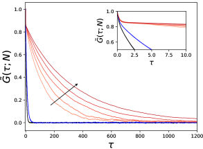
(a)

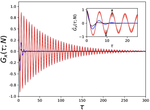
(b)

Figure 1: Renormalised response functions as a function of time $\tau$. Panel LABEL:sub@fig:_subfig_1a: response $\tilde{G}(\tau;N)$ for the one dimensional order parameter of the DZ model. Panel LABEL:sub@fig:_subfig_1b: response $\tilde{G}_{x}(\tau;N)$ of the first component of the bi-dimensional order parameter for the BCM model. Black and blue lines correspond to non critical values of the strength of the noise $\sigma$. Red lines correspond to response functions at the transition point. For each value of $\sigma$, there are five lines corresponding to different values of $N$, namely $N=2^{k}\times 10^{3}$ with $k=1,\dots,5$. The arrows and the colour gradient indicate the direction of increasing $N$.

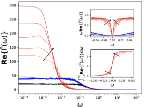
(a)

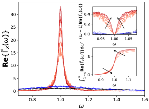
(b)

Figure 2: Macroscopic susceptibilities as a function of the frequency $\omega$. Panel LABEL:sub@fig:_subfig_2a: susceptibility $\tilde{\Gamma}(\omega)$ for the one dimensional order parameter of the DZ model. Panel LABEL:sub@fig:_subfig_2b: susceptibility $\tilde{\Gamma}_{x}(\omega)$ for the first component of the two dimensional order parameter for the BCM model. The parameter in the lower extreme of the integral is for both cases $c=0.05$. Blue and black lines in panel 2b have been multiplied by a factor $5$ for visualisation purposes. Colour code and plotting conventions as in Figure 1.

As discussed in Lucarini, Pavliotis, and Zagli (2020), the critical behaviour of this class of multiagent systems, signified by the singular behaviour of the susceptibility, originates from two distinct physical phenomena that are associated to either the poles of $\Gamma_{i}(\omega)$ or $P_{ij}^{-1}(\omega)$. The case where $\Gamma_{i}(\omega)$ diverges pertains to the occurrence of critical transitions.
It is of interest here the case where poles appear in the real $\omega$ axis for $\tilde{\Gamma}_{i}(\omega)$ because the matrix $P^{-1}_{ij}(\omega)$ becomes singular. This corresponds to phase transitions originated by the coupling and do not show a divergence of correlation properties, because $\Gamma_{i}(\omega)$ is, instead, analytic in the upper complex $\omega$ plane. Equivalently, the spectral gap of $\mathcal{L}^{+}_{\langle x\rangle_{0}}$ remains finite at a phase transition. However, at the transition point, the usual dispersion relations need to be modified Lucarini, Pavliotis, and Zagli (2020); Lucarini et al. (2005). The conditions underpinning the breakdown of linear response theory do not depend on the perturbation field $\mathbf{X}(\mathbf{x})$ nor on the choice of the observable ($\mathbf{x}$, in our case) and can be related to the spectral properties of a modified transfer operator Lucarini, Pavliotis, and Zagli (2020).

III Numerical results

Below, we present results for the Desai-Zwanzig (DZ)  Desai and Zwanzig (1978) and the Bonilla-Casado-Morillo (BCM)  Bonilla, Casado, and Morillo (1987) models. These are composed by $N$ interacting agents evolving according to Eq. 1. Each individual agent of the DZ (BCM) model evolves in $\mathbb{R}$ ($\mathbb{R}^{2}$). A detailed description of the two models is presented in the Appendix. We repeat our experiments for various choices of $N$, in order to detect the emergence of singularities for the combination of the parameters corresponding to phase transitions. Here, we keep fixed the values of the internal parameter $\alpha$. Both models undergo a phase transition at the transition line $\tilde{\sigma}=\sigma(\theta;\alpha)$ in the parameter space $(\sigma,\theta)$, see Appendix for the analytical evaluation of the transition line. Since one of the two parameters is redundant, we fix the coupling intensity $\theta$ and we vary, instead, the noise strength $\sigma$.

Following Marconi et al. (2008b), we perform $n$ simulations where the initial conditions are chosen according to the unperturbed invariant measure $\rho_{0}(\mathbf{x})$ and where at time $\tau=0$ we apply a perturbation proportional to a Dirac $\delta$ function. The average of the response for the observable $\mathbf{x}$ over the $n$ simulations gives an estimate $\tilde{G}_{i}(\tau;N)$ of the renormalised response function . Details on the numerical simulations are also reported in the Appendix. Figure 1 shows the response functions $\tilde{G}_{i}(\tau;N)$ for an additive perturbation $\mathbf{X}(\mathbf{x})=1$ for the DZ model (left panel) and $\mathbf{X}(\mathbf{x})=(1,0)$ for the BCM model (right panel). The two response functions are qualitatively different because, by and large, the one for the DZ model describes a monotonic decay, whereby the system relaxes towards the unperturbed state, while the one for the BCM combines the decay with an oscillatory behaviour taking place at the natural frequency $\tilde{\omega}=1$.

In the DZ model, the response functions initially undergo a fast and substantial decay, both far from and at the phase transition, associated with a time scale of order $1$. However, at the phase transition, a new, much longer, timescale appears. This timescale increases monotonically with $N$. The same is observed in the case of the BCM model if one considers the envelope of the response function rather than the response function itself: at the transition the decay of the oscillations becomes slower and slower as $N$ increases.
The origin of the new timescales resides in the appearance of simple pole at $\omega=\omega_{0}$ in the susceptibility $\tilde{\Gamma}_{i}(\omega;N)$, the Fourier transform of the response function. The pole is located at $\omega_{0}=0$ for the DZ model and at $\omega_{0}=\tilde{\omega}=1$ for the BCM model. When considering finite values of $N$, the susceptibilities describing the response of (virtually) any observable to (virtually) any external perturbation have a contribution of the form $\frac{\kappa}{\omega-\omega_{0}+i\gamma(N)}$, where $\gamma(N)\rightarrow 0^{+}$ as $N\rightarrow+\infty$ and $\kappa$ represents the residue of the pole, because $\lim_{N\rightarrow\infty}\frac{\kappa}{\omega-\omega_{0}+i\gamma(N)}=-i\pi\kappa\delta(\omega-\omega_{0})+\kappa\mathcal{P}(1/(\omega-\omega_{0}))$. The quantity $\kappa\in\mathbb{C}$ depends on the choice of observable and of the perturbation. We remark that the asymptotic property does not depend on how fast the function $\gamma(N)$ vanishes for increasing values of $N$. Following Delgadino, Gvalani, and Pavliotis (2021), one might conjecture that for the Desai-Zwanzig model and related models the function $\gamma$ would scale as $1/N$. Instead, we have observed here that the behaviour of $\gamma$ is different. This is an issue of fundamental importance that we will explore in future work, also in the case of nonequilibrium systems. Note also that, in the case of equibrium systems, the mean field limit $N\rightarrow\infty$ and the limit $T\rightarrow T_{c}$, where $T_{c}$ is the critical temperature, do not commute Chavanis (2014).

We next investigate the phase transitions by looking at the properties of the susceptibilities, see Fig. 2. When $\sigma\neq\tilde{\sigma}$, the susceptibilities do not show any singularity nor any remarkable dependence on $N$, thus indicating that the thermodynamic limit has been reached to a good approximation. As $N$ increases, for both the DZ model (left panel) and the BCM model (right panel) the resonance at $\omega=\omega_{0}$ of the real part of the susceptibility approaches the limiting Dirac function $\pi k\delta(\omega-\omega_{0})$ with coefficient $k>0$. This singular behaviour is clear from the plot of the primitive function of the real part of the susceptibility (bottom inset) that tends to step function. For both models $\kappa=\mathrm{i}k$ is an imaginary number. Indeed, the imaginary part of the susceptibility behaves exactly as the Cauchy principal value distribution and can be used to get easily a quantitative estimate of $k$. The top insets of Figure 2 shows the function $(\omega-\omega_{0})\mathbf{Im}\{\tilde{\Gamma}_{i}(\omega)\}$. As $N\rightarrow\infty$, this function converges to $k$ everywhere except for $\omega=\omega_{0}$.
An explicit expression for $k$ is known Lucarini, Pavliotis, and Zagli (2020) in the case of the DZ model $k=\frac{\langle x^{2}\rangle_{0}}{\theta\int_{0}^{+\infty}\mathrm{d}t\langle x(t)x(0)\rangle_{0}}$. Using the statistics of the unperturbed runs we obtain $k\approx 0.89$, which agrees within 2% with the one obtained from the limiting behaviour of the susceptibility, thus validating our results. In the case of the BCM model, our procedure allows one to derive a direct estimate $k\approx 0.44$; in this case no expression for the residue is available in the literature and, following Bonilla, Casado, and Morillo (1987); Lucarini, Pavliotis, and Zagli (2020), its evaluation seems cumbersome. We here observe that, by evaluating the susceptibility for finite values of $N$, we are able to predict the residue of the pole at $\omega=\omega_{0}$, which appears, instead, only in the thermodynamic limit. The residue plays the role of a latent heat of phase change in classical thermodynamics. Our results, though, allow one to deal with the case of a dynamical latent heat, that is observed for perturbations occurring a non-vanishing frequency. As discussed earlier, the singular behaviour of the susceptibility has some degree of universality. By this we mean that while for a given model the value of the residue is forcing- and observable-dependent, its position is a fundamental property of the model itself; see the Appendix for an additional examples.

IV Conclusions

The study of how a large network of identical agents respond to exogenous perturbations is of the uttermost importance in different areas of science. One might be interested not only in the smooth response of the system, where its properties change ever so slightly, but also in the critical, nonsmooth, regime, where small perturbations can lead to large and possibly undesired changes. Multiagent systems modeled as weakly interacting Itô diffusions represent a rich class of models exhibiting such critical behaviour, and for which rigorous analysis and careful numerical investigations can be carried out. Usually these phenomena are accompanied by a large spatial (among sub-systems) and temporal restructuring of the system where correlations get highly magnified. The critical behaviour due to the emergence of a phase transition is a genuine thermodynamic phenomenon arising from the complex interactions among the infinite number of agents. Nevertheless, we have shown in this paper that linear response theory provides a powerful framework for detecting and anticipating phase transitions by investigating the response of a finite particle system to external perturbations.We have been able to predict the appearance of poles in the susceptibility, which describes the frequency-dependent response of the system, as well as to obtain a correct estimate of critical thermodynamic properties, such as the residue of the poles, based on the knowledge of the response for the finite particle system in two paradigmatic models describing equilibrium and nonequilibrium phase transitions. This is an encouraging starting point for improving our ability to understand and predict transitions in more complex multiagent systems.

Data Availability

The data that support the findings of this study are openly available in "Spectroscopy of Phase Transitions" at https://figshare.com/projects/Spectroscopy_of_phase_transitions/101846, reference number Zagli (2021).

Appendix A The models

Weakly interacting diffusions represent a rich class of agent based models, describing a network of interacting subsystems. The local dynamics of each subsystem is determined by a smooth vector field $\mathbf{F}_{\alpha}(\mathbf{x})$. The local force is in general non conservative, leading to irreversible and dissipative processes that can exhibit complex behaviours, such as deterministic chaos, see Figure 3.

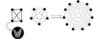
Figure 3: Weakly interacting diffusions. The local dynamics of each subsystem, given by $\mathbf{F}_{\alpha}(\mathbf{x})$, is in general dissipative and can support a wide range of complex behaviours, including deterministic chaos, as depicted in this figure.

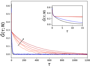
(a)

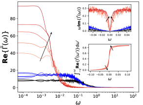
(b)

Figure 4: Panel LABEL:sub@fig:_subfig_3a: Response function $\tilde{G}(\tau;N)$ and Panel LABEL:sub@fig:_subfig_3b: susceptibility $\tilde{\Gamma}(\omega;N)$ for a spatially dependent perturbation $\mathbf{X}(\mathbf{x})=x^{2}$ for the one dimensional order parameter for the DZ model. Colour code and plotting conventions as in Figure 1. The lower extreme of the integral of the bottom panel is $c=0.05$.

An all-to-all coupling between the subsystems is given by a matrix $L_{ij}=\mathbf{\nabla}\mathcal{U}(\mathbf{x}^{i}-\mathbf{x}^{j})$ where $\mathcal{U}(\mathbf{x})=\mathcal{U}(-\mathbf{x})$ represents the interaction potential and $\mathbf{x}^{i}$ is the state vector of the $i$-th subsystem. Weakly interacting diffusions are characterised by a coupling strength which is inversely proportional to the number of subsystems $N$. As $N$ increases, the interaction structure gets more and more intricate, while the intensity becomes weaker and weaker, see Figure 3. As mentioned in the main text, the DZ model has been introduced, and thereafter commonly used, as a paradigmatic example of an equilibrium continuous phase transition reminiscent of the Ising-like ferromagnetic transitions in spin systems Dawson (1983); Shiino (1987). The DZ model describes a network of one-dimensional subsystems $x^{k}$ whose dynamics is prescribed by the following equations (see main text for notation)

$$\mathrm{d}x^{k}=-V^{\prime}_{\alpha}(x^{k})\mathrm{d}t-\frac{\theta}{N}\sum_{l=1}^{N}\left(x^{k}-x^{l}\right)\mathrm{d}t+\sigma\mathrm{d}W^{k}$$ (6)

where $k=1,\dots,N$ and the confining potential $V_{\alpha}(x)=-\frac{\alpha}{2}x^{2}+\frac{x^{4}}{4}$ has a double well shape for $\alpha>0$. Without loss of generality, we here consider $\alpha=1$. In the absence of coupling, $\theta=0$, the above equations describe the simple motion of a particle in a double well potential, subject to additive noise. The presence of the coupling allows for a long range coordination of the system that in the thermodynamic limit $N\rightarrow+\infty$ results in a proper phase transition. In this regime, by varying the parameters $(\alpha,\theta)$, the order parameter $\langle x\rangle$ undergoes a continuous order-disorder transition, similar to the pitchfork bifurcation diagram for the Ising model. It is possible to show Dawson (1983) that the critical line is given by $\frac{D_{-3/2}\left(\frac{\theta-1}{\sigma}\right)}{D_{-1/2}\left(\frac{\theta-1}{\sigma}\right)}=\frac{\sigma}{\theta}$ where $D_{\nu}(z)$ is a parabolic cylinder function. Here the coupling $\theta$ is kept fixed ($\theta=0.55$) and we vary $\sigma$ to approach the transition point.

The BCM model describes an ensemble of bi-dimensional nonlinear oscillators undergoing an out of equilibrium self-synchronisation transition. The time evolution of the network of oscillators is given by the following equations

$$\mathrm{d}\mathbf{x}^{k}=\mathbf{F}_{\alpha}(\mathbf{x}^{k})\mathrm{d}t-\frac{\theta}{N}\sum_{l=1}^{N}\left(\mathbf{x}^{k}-\mathbf{x}^{l}\right)\mathrm{d}t+\sigma\mathrm{d}\mathbf{W}^{k},$$ (7)

where the local force is not conservative, giving rise to the non equilibrium features of the system, and reads $\mathbf{F}_{\alpha}(\mathbf{x})=\left(\alpha-|\mathbf{x}|^{2}\right)\mathbf{x}+\mathbf{x}^{+}$where $\mathbf{x}^{+}=(-x_{2},x_{1})$. The latter term corresponds to a rotation and makes the stationary state a non equilibrium one. The parameter $\alpha>0$ controls the amplitude of the oscillations of the individual non linear oscillators. In fact, when $\theta=\sigma=0$, each subsystem oscillates as $\mathbf{x}^{j}(t)=\sqrt{\alpha}\left(\cos(t+\beta_{j}),\sin(t+\beta_{j})\right)$ where $\beta_{j}=\tan(x^{j}_{2}(0)/x^{j}_{1}(0))$. The coupling tries to synchronise the subsystems by attracting them towards the center of mass $\frac{1}{N}\sum_{j=1}^{N}\mathbf{x}^{j}$. In the thermodynamic limit and for sufficiently low values of the noise, the order parameter $\langle\mathbf{x}\rangle=\langle\mathbf{x}\rangle(t)$ exhibits a periodic time evolution, resulting from the subsystem oscillating in a coherent way. On the other hand, high values of the noise correspond to a non synchronised state where the order parameter vanishes. In particular, the transition happen at the surface of the $(\alpha,\theta,\sigma)$ parametric space defined by Bonilla, Casado, and Morillo (1987)

$$A=\frac{\delta^{2}}{2}\left[1-\frac{1}{\delta}\exp\left(-\frac{A^{2}}{\delta^{2}}\right)\left[\int_{-\frac{A}{\delta}}^{\infty}e^{-r^{2}}dr\right]^{-1}\right]$$ (8)

where $A=\frac{\alpha}{\theta}-1$ and $\delta=\frac{\sqrt{2\sigma^{2}}}{\theta}$. In the following we have $\theta=\alpha=2$. The colour code for the figures is given by:

• non critical black : DZ $\sigma\approx 1$ , BCM $\sigma\approx 2$.

• non critical blue : DZ $\sigma\approx 0.87$ , BCM $\sigma\approx 1.8$

• critical red : DZ $\tilde{\sigma}\approx 0.75$ , BCM $\tilde{\sigma}\approx 1.59$.

A.1 Numerical linear response experiments

As mentioned in the main text, we perform $n$ simulations of the response given by Eqs. 6 and 7 where the initial conditions are chosen according to the respective unperturbed invariant measure $\rho_{0}(\mathbf{x})$ and where at time $\tau=0$ we apply a perturbation proportional to a Dirac’s $\delta(\tau=0)$. The average of the response for the observable $\mathbf{x}$ over the $n$ simulations gives an estimate of $\tilde{G}_{i}(\tau;N)$. The response functions away from the transitions are estimated on an ensemble of $n=10^{5}$ simulations, while the critical response functions with $n=10^{6}$ for DZ and $n=7\times 10^{6}$ for BCM. Furthermore we investigate the response up to time $\tau=5\times 10^{3}$. The corresponding susceptibility $\tilde{\Gamma}_{i}(\omega;N)$ is simply defined as the Fourier Transform of $\tilde{G}_{i}(\tau;N)$. In the main text, we show the results for an additive perturbation $\mathbf{X}(\mathbf{x})\equiv\mathbf{X}$. However, the critical behaviour of the response does not depend on the type of perturbation, modulo a potential degenerate class of perturbations that have zero projection on the invariant measure $\rho_{0}(\mathbf{x})$. We have thus decided to investigate the response of the DZ model for a spatially dependent perturbation $X(x)=x^{2}$, see Figure 4. The response function $\tilde{G}_{i}(\tau;N)$, both away and at the phase transition, has a rapid initial decay with a timescale that is different from the response function shown in the main text. As a matter of fact, the timescale associated to the dominant mode of the response function for $\tau\rightarrow 0$ does in general depend on the applied perturbation Lucarini, Pavliotis, and Zagli (2020). As expected, the response function at the phase transition develops a much longer timescale that increases as the number of particle increases. A more accurate comparison with the result shown in the main text can only be performed in the frequency domain. Figure 4 (right panel) shows that, away from the transition, the susceptibilities have a smooth behaviour and no evident dependence on $N$. At the phase transition, the susceptibility develops the expected singular behaviour $\frac{\kappa}{\omega-\omega_{0}+i\gamma(N)}$, where $\gamma(N)\rightarrow 0^{+}$ as $N\rightarrow+\infty$ due to the appearance of a simple pole $\omega_{0}=0$. The residue $\kappa$ is purely imaginary and its magnitude $k$ can be inferred by visual inspection of the top inset representing the function$(\omega-\omega_{0})\mathbf{Im}\{\tilde{\Gamma}(\omega)\}$ to be just less than 0.29. As mentioned in the main text, the residue depends both on the observable and on the perturbation $\mathbf{X}(\mathbf{x})$.

References

- Naldi, Pareschi, and Toscani (2010) G. Naldi, L. Pareschi, and G. Toscani, Mathematical Modeling of Collective Behavior in Socio-Economic and Life Sciences (Birkhäuser Basel, 2010).
- Pareschi and Toscani (2013) L. Pareschi and G. Toscani, “Interacting multiagent systems: kinetic equations and monte carlo methods,” (2013).
- Dawson (1983) D. A. Dawson, “Critical dynamics and fluctuations for a mean-field model of cooperative behavior,” J. Stat. Phys. 31, 29–85 (1983).
- Acebrón et al. (2005) J. A. Acebrón, L. L. Bonilla, C. J. Pérez Vicente, F. Ritort, and R. Spigler, “The kuramoto model: A simple paradigm for synchronization phenomena,” Rev. Mod. Phys. 77, 137–185 (2005).
- Garnier, Papanicolaou, and Yang (2013) J. Garnier, G. Papanicolaou, and T. Yang, “Large deviations for a mean field model of systemic risk,” SIAM Journal on Financial Mathematics 4, 151–184 (2013), https://doi.org/10.1137/12087387X .
- Wang et al. (2017) C. Wang, Q. Li, W. E, and B. Chazelle, “Noisy hegselmann-krause systems: Phase transition and the 2r-conjecture,” J. Stat. Phys. 166, 1209–1225 (2017).
- Garnier, Papanicolaou, and Yang (2017) J. Garnier, G. Papanicolaou, and T. Yang, “Consensus convergence with stochastic effects,” Vietnam Journal of Mathematics 45, 51–75 (2017).
- Garbuno-Inigo, Nüsken, and Reich (2020) A. Garbuno-Inigo, N. Nüsken, and S. Reich, “Affine invariant interacting Langevin dynamics for Bayesian inference,” SIAM J. Appl. Dyn. Syst. 19, 1633–1658 (2020).
- Simmonds, Gómez, and Ledezma (2019) J. Simmonds, J. A. Gómez, and A. Ledezma, “The role of agent-based modeling and multi-agent systems in flood-based hydrological problems: a brief review,” Journal of Water and Climate Change (2019), 10.2166/wcc.2019.108, jwc2019108, https://iwaponline.com/jwcc/article-pdf/doi/10.2166/wcc.2019.108/625177/jwc2019108.pdf .
- Geisendorf (2018) S. Geisendorf, “Evolutionary climate-change modelling: A multi-agent climate-economic model,” Computational Economics 52, 921–951 (2018).
- Scheffer (2009) M. Scheffer, Critical Transitions in Nature and Society, Princeton Studies in Complexity (Princeton University Press, Princeton, 2009).
- Sornette (0006) D. Sornette, “Endogenous versus exogenous origins of crises,” in Extreme Events in Nature and Society, edited by K. H. Albeverio S., Jentsch V. (, Berlin, Heidelberg, 20006) pp. 95–119.
- Kubo (1966) R. Kubo, “The fluctuation-dissipation theorem,” Reports on Progress in Physics 29, 255–284 (1966).
- Marconi et al. (2008a) U. M. B. Marconi, A. Puglisi, L. Rondoni, and A. Vulpiani, “Fluctuation–dissipation: Response theory in statistical physics,” Physics Reports 461, 111 – 195 (2008a).
- Baiesi and Maes (2013) M. Baiesi and C. Maes, “An update on the nonequilibrium linear response,” New Journal of Physics 15, 013004 (2013).
- Sarracino and Vulpiani (2019) A. Sarracino and A. Vulpiani, “On the fluctuation-dissipation relation in non-equilibrium and non-hamiltonian systems,” Chaos: An Interdisciplinary Journal of Nonlinear Science 29, 083132 (2019), https://doi.org/10.1063/1.5110262 .
- Lucarini et al. (2005) V. Lucarini, J. J. Saarinen, K.-E. Peiponen, and E. M. Vartiainen, Kramers-Kronig relations in Optical Materials Research (Springer, New York, 2005).
- Binney and Tremaine (2008) J. Binney and S. Tremaine, Galactic Dynamics, 2nd ed. (Princeton University Press, Princeton, 2008).
- Leith (1975) C. E. Leith, “Climate response and fluctuation dissipation,” J. Atmos. Sci. 32, 2022 (1975).
- North, Bell, and Hardin (1993) G. North, R. Bell, and J. Hardin, “Fluctuation dissipation in a general circulation model,” Clim. Dyn. 8, 259 (1993).
- Öttinger (2005) H. Öttinger, Beyond Equilibrium Thermodynamics (Wiley, Hoboken, 2005).
- Lucarini, Ragone, and Lunkeit (2017) V. Lucarini, F. Ragone, and F. Lunkeit, “Predicting climate change using response theory: Global averages and spatial patterns,” J. Stat. Phys. 166, 1036–1064 (2017).
- Cessac (2019) B. Cessac, “Linear response in neuronal networks: From neurons dynamics to collective response,” Chaos 29, 103105 (2019).
- Gottwald (2020) G. A. Gottwald, “Introduction to focus issue: Linear response theory: Potentials and limits,” Chaos: An Interdisciplinary Journal of Nonlinear Science 30, 020401 (2020), https://doi.org/10.1063/5.0003135 .
- Ruelle (1998) D. Ruelle, “Nonequilibrium statistical mechanics near equilibrium: computing higher-order terms,” Nonlinearity 11, 5–18 (1998).
- Ruelle (2009) D. Ruelle, “A review of linear response theory for general differentiable dynamical systems,” Nonlinearity 22, 855–870 (2009).
- Baladi (2014) V. Baladi, “Linear response, or else,” in ICM Seoul 2014, Proceedings, Vol. III (2014) p. 525–545.
- Dembo and Deuschel (2010) A. Dembo and J.-D. Deuschel, “Markovian perturbation, response and fluctuation dissipation theorem,” Ann. Inst. Henri Poincaré Probab. Stat. 46, 822–852 (2010).
- Hairer and Majda (2010) M. Hairer and A. J. Majda, “A simple framework to justify linear response theory,” Nonlinearity 23, 909–922 (2010).
- Wormell and Gottwald (2019) C. L. Wormell and G. A. Gottwald, “Linear response for macroscopic observables in high-dimensional systems,” Chaos: An Interdisciplinary Journal of Nonlinear Science 29, 113127 (2019).
- Liverani and Gouëzel (2006) C. Liverani and S. Gouëzel, “Banach spaces adapted to Anosov systems,” Ergodic Theory and Dynamical Systems 26, 189–217 (2006).
- Chekroun et al. (2014) M. D. Chekroun, J. D. Neelin, D. Kondrashov, J. C. McWilliams, and M. Ghil, “Rough parameter dependence in climate models and the role of Ruelle-Pollicott resonances,” Proceedings of the National Academy of Sciences 111, 1684–1690 (2014).
- Lucarini (2016) V. Lucarini, “Response operators for Markov processes in a finite state space: Radius of convergence and link to the response theory for Axiom A systems,” J. Stat. Phys. 162, 312–333 (2016).
- Tantet, Lucarini, and Dijkstra (2018) A. Tantet, V. Lucarini, and H. A. Dijkstra, “Resonances in a Chaotic Attractor Crisis of the Lorenz Flow,” J. Stat. Phys. 170, 584–616 (2018), arXiv:1705.08178 .
- Pollicott (1985) M. Pollicott, “On the rate of mixing of Axiom A flows,” Inventiones Mathematicae 81, 413–426 (1985).
- Ruelle (1986) D. Ruelle, “Resonances of chaotic dynamical systems,” Physical Review Letters 56, 405–407 (1986).
- Shiino (1987) M. Shiino, “Dynamical behavior of stochastic systems of infinitely many coupled nonlinear oscillators exhibiting phase transitions of mean-field type: H theorem on asymptotic approach to equilibrium and critical slowing down of order-parameter fluctuations,” Phys. Rev. A 36, 2393–2412 (1987).
- Delgadino, Gvalani, and Pavliotis (2021) M. G. Delgadino, R. S. Gvalani, and G. A. Pavliotis, “On the diffusive-mean field limit for weakly interacting diffusions exhibiting phase transitions,” Archive for Rational Mechanics and Analysis (2021), 10.1007/s00205-021-01648-1.
- Carrillo et al. (2020) J. A. Carrillo, R. S. Gvalani, G. A. Pavliotis, and A. Schlichting, “Long-time behaviour and phase transitions for the McKean-Vlasov equation on the torus,” Arch. Ration. Mech. Anal. 235, 635–690 (2020).
- Lucarini, Pavliotis, and Zagli (2020) V. Lucarini, G. A. Pavliotis, and N. Zagli, “Response theory and phase transitions for the thermodynamic limit of interacting identical systems,” Proc. R. Soc. A. 476 (2020), https://doi.org/10.1098/rspa.2020.0688 .
- Jackson (1975) J. D. Jackson, Classical electrodynamics; 2nd ed. (Wiley, New York, NY, 1975).
- Talebian and Talebian (2013) E. Talebian and M. Talebian, “A general review on the derivation of clausius-mossotti relation,” Optik 124, 2324 – 2326 (2013).
- Sornette and Helmstetter (2003) D. Sornette and A. Helmstetter, “Endogenous versus exogenous shocks in systems with memory,” Physica A: Statistical Mechanics and its Applications 318, 577 – 591 (2003).
- Yoshida (2003) N. Yoshida, “Phase transition from the viewpoint of relaxation phenomena,” Rev. Math. Phys. 15, 765–788 (2003).
- Desai and Zwanzig (1978) R. C. Desai and R. Zwanzig, “Statistical mechanics of a nonlinear stochastic model,” J. Stat. Phys. 19, 1–24 (1978).
- Bonilla, Casado, and Morillo (1987) L. L. Bonilla, J. Casado, and M. Morillo, “Self-synchronization of populations of nonlinear oscillators in the thermodynamic limit,” J. Stat. Phys. 48, 571–591 (1987).
- Sznitman (1989) A. Sznitman, Topics in propagation of chaos., Hennequin PL. (eds) Ecole d’Eté de Probabilités de Saint-Flour XIX — 1989. Lecture Notes in Mathematics, Vol. 1464 (Springer, Berlin, Heidelberg, 1989).
- Oelschlager (1984) K. Oelschlager, “A martingale approach to the law of large numbers for weakly interacting stochastic processes,” Ann. Probab. 12, 458–479 (1984).
- Dawson and Gärtner (1987) D. A. Dawson and J. Gärtner, “Large deviations from the McKean-Vlasov limit for weakly interacting diffusions,” Stochastics 20, 247–308 (1987).
- Helffer (2002) B. Helffer, Semiclassical analysis, Witten Laplacians, and statistical mechanics, Series in Partial Differential Equations and Applications, Vol. 1 (World Scientific Publishing Co., Inc., River Edge, NJ, 2002) pp. x+179.
- Frank (2004) T. Frank, “Fluctuation–dissipation theorems for nonlinear Fokker–Planck equations of the Desai–Zwanzig type and Vlasov–Fokker–Planck equations,” Physics Letters A 329, 475 – 485 (2004).
- Chekroun et al. (2020) M. D. Chekroun, A. Tantet, H. A. Dijkstra, and J. D. Neelin, “Ruelle–pollicott resonances of stochastic systems in reduced state space. part i: Theory,” J. Stat. Phys. (2020), 10.1007/s10955-020-02535-x.
- Lasota and Mackey (1994) A. Lasota and M. C. Mackey, Chaos, fractals, and noise, 2nd ed., Applied Mathematical Sciences, Vol. 97 (Springer-Verlag, New York, 1994) pp. xiv+472.
- Marconi et al. (2008b) U. M. B. Marconi, A. Puglisi, L. Rondoni, and A. Vulpiani, “Fluctuation-dissipation: Response theory in statistical physics,” Phys. Rep. 461, 111 (2008b).
- Chavanis (2014) P.-H. Chavanis, “The brownian mean field model,” The European Physical Journal B 87, 120 (2014).
- Note (1) There is a typo in the formula given in Lucarini, Pavliotis, and Zagli (2020). Furthermore, the convention for the Fourier transform we use here has the opposite sign, ditto the residue.
- Zagli (2021) N. Zagli, “Spectroscopy of phase transitions,” Figshare (2021).