Skye: A Differentiable Equation of State

Abstract

Stellar evolution and numerical hydrodynamics simulations depend critically on access to fast, accurate, thermodynamically consistent equations of state. We present Skye, a new equation of state for fully-ionized matter. Skye includes the effects of positrons, relativity, electron degeneracy, Coulomb interactions, non-linear mixing effects, and quantum corrections. Skye determines the point of Coulomb crystallization in a self-consistent manner, accounting for mixing and composition effects automatically. A defining feature of this equation of state is that it uses analytic free energy terms and provides thermodynamic quantities using automatic differentiation machinery. Because of this, Skye is easily extended to include new effects by simply writing new terms in the free energy. We also introduce a novel thermodynamic extrapolation scheme for extending analytic fits to the free energy beyond the range of the fitting data while preserving desirable properties like positive entropy and sound speed. We demonstrate Skye in action in the MESA stellar evolution software instrument by computing white dwarf cooling curves.

1 Introduction

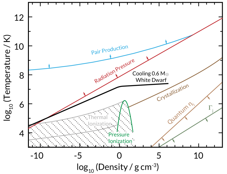
Figure 1: Coverage of the Skye EOS in the ($\rho,T$) plane. Shown is approximately where radiation pressure (red) dominates the gas pressure, thermodynamics from $e^{-}e^{+}$ pair production (light blue) dominates, crystallization of ions (brown) begins, thermal (light gray) and pressure (green) ionization of atoms occurs. Lines of constant ion quantum parameter $\eta_{j}$ (light brown) and ion interaction strength $\Gamma_{j}$ (dark green) are indicated in the lower-right, and attached arrows denote directions of increasing $\eta_{j}$ and $\Gamma_{j}$. The dotted region marks where Skye’s assumption of full ionization is a poor approximation. An example profile, from core to surface, of a cooling white dwarf (black) is illustrated.

The equation of state (EOS) of ionized matter is a key ingredient in models of stars, gas giant planets, accretion disks, and many other astrophysical systems. These applications span many orders of magnitude in both density and temperature, and include both low-density systems that are thermally ionized (e.g., stellar atmospheres) and high-density ones that are pressure-ionized (e.g., planetary interiors). Moreover matter can have many different compositions, ranging from pure hydrogen to exotic mixtures of heavy metals. As a result, approximations to nature’s EOS of ionized matter must capture a wide variety of physics (Figure 1) including relativity, quantum mechanics, electron degeneracy, pair production, phase transitions, and chemical mixtures.

Despite these challenges, several different equations of state have been introduced for ionized matter (e.g., Salpeter, 1961; Eggleton et al., 1973; Bludman & van Riper, 1977; Daeppen et al., 1990; Pols et al., 1995; Rogers et al., 1996; Blinnikov et al., 1996; Timmes & Arnett, 1999; Gong et al., 2001a; Däppen, 2010). Chabrier (1990) introduced an EOS for non-relativistic ionized hydrogen, incorporating sophisticated quantum and electron screening corrections. Improvements then led to the PC EOS (Chabrier & Potekhin, 1998; Potekhin & Chabrier, 2000; Potekhin et al., 2009; Potekhin & Chabrier, 2010). PC allows for arbitrary compositions and incorporates relativistic ideal electrons as well as modern prescriptions for electron screening and multi-component plasmas. Potekhin & Chabrier (2013) extended the PC EOS to include the effects of strong magnetic fields such as those found in neutron stars. One of the distinguishing features of the PC EOS is the use of analytic prescriptions to capture non-ideal physics.

One of the limitations of the PC EOS is that it does not capture the effects of electron-positron pair production at high temperatures, which is important for the pair instability in massive stars (Rakavy & Shaviv, 1967). The treatment of electron degeneracy and the ideal quantum electron gas is also approximate, based on fitting formulas which approximate the relevant Fermi integrals. These limitations are addressed by the HELM EOS (Timmes & Swesty, 2000). While HELM does not include the sophisticated non-ideal corrections which are a defining strength of PC, it provides a tabulated Helmholtz free energy treatment of an ideal quantum electron-positron plasma, obtained by high-precision evaluation of the relevant Fermi-Dirac integrals (Cloutman, 1989; Aparicio, 1998; Gong et al., 2001b). As such, HELM accurately and efficiently handles relativistic effects, degeneracy effects, and high-temperature pair production.

In this article we build on this progress by presenting a new equation of state, Skye, an EOS designed to handle density and temperature inputs over the range $10^{-12}\,\mathrm{g\,cm^{-3}}<\rho<10^{13}\,\mathrm{g\,cm^{3}}$ and $10^{3}\,\mathrm{K}<T<10^{13}\,\mathrm{K}$ (Figure 1). Skye assumes material is fully-ionized, so the suitability of the result is subject to the (composition-dependent) constraint that material is either pressure-ionized ($\rho\gtrsim 10^{3}\,\mathrm{g\,cm^{-3}}$) or thermally-ionized ($T\gtrsim 10^{5}\,\mathrm{K}$). Further limits to Skye’s suitability can arise due to violations of its other physics assumptions. Building on HELM, we use the full ideal equation of state for electrons and positrons, accounting for degeneracy and relativity. Ions are assumed to be a classical ideal gas. We then add non-ideal classical and quantum corrections to account for electron-electron, electron-ion, and ion-ion interactions following a multi-component ion plasma prescription. These corrections are generally similar to those used by the PC EOS, though we have used updated physics prescriptions in some instances (e.g., those of Baiko, 2019).

Thermodynamic quantities in Skye are derived from a Helmholtz free energy to ensure thermodynamic consistency. Automatic differentiation machinery allows extraction of arbitrary derivatives from an analytic Helmholtz free energy, allowing Skye to provide the high-order derivatives needed for stellar evolution calculations (e.g., Paxton et al., 2011). We further leverage this machinery to make the EOS easily extensible: adding new or refined physics to Skye is as easy as writing a formula for the additional Helmholtz free energy. The often painstaking and error-prone process of taking and programming analytic first, second, and even third derivatives of the Helmholtz free energy is eliminated. In this way Skye is a framework for rapidly developing and prototyping new EOS physics as advances are made in numerical simulations and analytic calculations. We emphasize that Skye is not tied to a specific set of physics choices; Skye in 10 years is unlikely to be the same as Skye as described in this article.

In addition to being a single EOS which can be used at both high temperatures, like HELM, and high densities, like PC, Skye currently includes two significant physical improvements. First, whereas PC fixes the location of Coulomb crystallization of the ions, Skye picks between the liquid and solid phase to minimize the Helmholtz free energy. This enables a self-consistent treatment of the phase transition, albeit one currently without chemical phase separation, and means that the Helmholtz free energy is continuous across the transition. Secondly, we introduce the technique of thermodynamic extrapolation, which provides a principled way to extend Helmholtz free energy fitting formulas beyond their original range of applicability and thus enables comparisons of the liquid and solid phase Helmholtz free energies.

This paper is structured as follows. Important symbols are defined in Table 1. In Section 2 we explain the various terms which contribute to the Helmholtz free energy in Skye, as well as the new handling of phase transitions (Section 2.2) and thermodynamic extrapolation (Section 2.3). Section 3 shows how we extract thermodynamic quantities from the Helmholtz free energy. We also introduce auxiliary quantities which allow stellar evolution software instruments to incorporate the latent heat of the Coulomb crystallization in a smooth manner. Section 4 discusses some of the current physics limitations of Skye, which is principally that it does not extend to cases of partially ionized or neutral matter, or dense nuclear matter (Hempel et al., 2012). Section 5 introduces our automatic differentiation machinery. In Section 6 we compare Skye to the PC and HELM equations of state and evaluate the quality of derivatives and thermodynamic consistency in Skye. We also calculate white dwarf cooling tracks and demonstrate that Skye properly accounts for the latent heat of crystallization (Section 6.5). In Section 7 we demonstrate that Skye has comparable runtime performance to PC, making it viable for use in stellar evolution calculations. Skye is open source and open-knowledge, and Section 8 describes options for obtaining and using Skye. We conclude with a discussion of future work in Section 9.

Table 1: Important symbols.

Name	Description	Appears
$T$	Temperature	1
$\rho$	Density	1
$F$	Helmholtz Free Energy	2
$F_{\rm ideal}$	Ideal Free Energy	2
$F_{\textrm{non-ideal}}$	Non-ideal Free Energy	2
$F_{\rm rad}$	Radiation Gas Free Energy	2.1
$F_{\rm ideal\ e^{-}e^{+}}$	Ideal Electron-Positron Free Energy	2.1
$F_{\rm ideal\ ion}$	Ideal Ion Free Energy	2.1
$F_{\rm ideal\ mix}$	Ideal Ion Mixing Free Energy	2.1
$a$	Radiation Gas Constant	2.1
$k_{\rm B}$	Boltzmann Constant	2.1
$m_{j}$	Mass of species $j$	2.1
$y_{j}$	Number fraction of ion species $j$	2.1
$\bar{m}$	Average ion mass	2.1
$n_{j}$	Number density of species $j$	2.1
$n_{Q,j}$	Quantum density of ion species $j$	2.1
$M_{\rm spin}$	Spin multiplicity of ion species $j$	2.1
$\hbar$	Reduced Planck Constant	2.1
$a_{j}$	Sphere radius of species $j$	2.2
	$(3n_{j}/4\pi)^{-1/3}$
$r_{s,j}$	Non-dimensional radius of species $j$	2.2
	$Z_{j}^{2}m_{j}e_{j}^{2}a_{j}/\hbar^{2}$
$Z_{j}$	Charge of species $j$	2.2
	($-1$ for electrons)
$\Gamma_{j}$	Coupling parameter of species $j$	2.2
	$Z_{j}^{2}e^{2}/a_{j}k_{\rm B}T$
$\eta_{j}$	Quantum Parameter of species $j$	2.2
	$(\hbar/k_{\rm B}T)\sqrt{4\pi e^{2}n_{j}Z_{j}^{2}/m_{j}}$
$p_{\rm F}$	Fermi Momentum	2.2
$x_{r}$	Relativity Parameter $p_{\rm F}/m_{e}c$	2.2
$\gamma$	Fermi Lorentz Factor	2.2
	$\sqrt{1+x_{r}^{2}}$
$E_{\rm F}^{\rm NR}$	Non-relativistic Fermi Energy	2.2
$h(\alpha)$	Switch function	2.2
$\alpha$	Switch parameter	2.2
	$3k_{\rm B}T\gamma/2E_{\rm F}^{\rm NR}$
$e$	Specific internal energy	2.3
$s$	Specific entropy	2.3
$T_{\rm b}$	Extrapolation Temperature	2.3
$\Gamma_{\rm max}^{\rm liquid}$	Liquid extrapolation $\Gamma_{j}$	2.3
$\Gamma_{\rm min}^{\rm solid}$	Solid extrapolation $\Gamma_{j}$	2.3
$p$	Pressure	3
$c_{v}$	Specific heat at constant volume	3
$c_{p}$	Specific heat at constant pressure	3
$\chi_{T}$	Thermal susceptibility	3
$\chi_{\rho}$	Density susceptibility	3
$\Gamma_{1}$	First adiabatic exponent	3
$\Gamma_{2}$	Second adiabatic exponent	3
$\Gamma_{3}$	Third adiabatic exponent	3
$\nabla_{\rm ad}$	Adiabatic Gradient	3
$c_{s}$	Sound speed	3
$\phi$	Smoothed phase parameter	3
$L_{T}$	Latent $Tds/d\ln T$	3
$L_{\rho}$	Latent $Tds/d\ln\rho$	3
$T_{j}^{\rm ion}$	Full-ionization $T$ of species $j$	4
$\rho_{j}^{\rm ion}$	Full-ionization $\rho$ of species $j$	4
$\rho_{j,\rm nuclear}$	Nuclear density of species $j$	4
$T_{\rm QCD}$	Temperature of	4
	proton rest mass-energy

2 Helmholtz Free Energy

The Skye equation of state is based on a Helmholtz free energy $F(\rho,T,\{n_{j}\})$ given by

$$F=F_{\rm ideal}+F_{\textrm{non-ideal}},$$ (1)

where $n_{j}$ is the number density of species $j$. Here $F$ is in terms of energy per unit mass. The ideal term incorporates all non-interacting contributions of relativistic electrons and positrons, non-relativistic non-degenerate ions, and photons. The non-ideal term contains the contributions of Coulomb interactions among and between electrons and ions.

2.1 Ideal Terms

The ideal free energy is

$$F_{\rm ideal}=F_{\rm rad}+F_{\rm ideal\ e^{-}e^{+}}+F_{\rm ideal\ ion}+F_{\rm ideal\ mix}.$$ (2)

$F_{\rm rad}$ is the free energy of an ideal gas of photons,

$$F_{\rm rad}=-\frac{aT^{4}}{3\rho},$$ (3)

where $a$ is the radiation gas constant.

$F_{\rm ideal\ e^{-}e^{+}}$ represents an ideal gas of non-interacting electrons and positrons, obtained from biquintic Hermite polynomial interpolation of a table (Timmes & Swesty 2000, also see Baturin et al. 2019). This single table captures both relativistic and degeneracy effects and is valid for any fully ionized composition.

$F_{\rm ideal\ ion}$ represents an ideal gas of non-degenerate ions and is given by (see e.g. Potekhin & Chabrier, 2010)

$$F_{\rm ideal\ ion}=\frac{k_{\rm B}T}{\bar{m}}\sum_{j}y_{j}\left[\ln\left(\frac{n_{j}}{n_{Q,j}}\right)-1\right],$$ (4)

where $y_{j}$ is the number fraction of species $j$,

$$\bar{m}\equiv\sum_{y}y_{j}m_{j}$$ (5)

is the mean ionic mass in $\mathrm{g}$, $m_{j}$ is the mass of ion species $j$, and

$$n_{Q,j}\equiv M_{\rm spin,j}\left(\frac{2\pi\hbar^{2}}{m_{j}k_{\rm B}T}\right)^{-3/2}.$$ (6)

Here $M_{\rm spin,j}$ is the spin multiplicity of the ion. The effect of $M_{\rm spin,j}$ is to introduce a composition-dependent offset in the entropy and so for simplicity we neglect it, setting $M_{\rm spin,j}=1$.

$F_{\rm ideal\ mix}$ captures the ideal free energy of mixing for ions, given by

$$F_{\rm ideal\ mix}=\frac{k_{\rm B}T}{\bar{m}}\sum_{j}y_{j}\ln y_{j}.$$ (7)

2.2 Non-Ideal Terms

The non-ideal free energy of electron interactions is commonly written in terms of the electron interaction strength

$$\Gamma_{e}\equiv\frac{e^{2}}{a_{e}k_{\rm B}T},$$ (8)

where

$$a_{e}\equiv\left(\frac{4}{3}\pi n_{e}\right)^{-1/3},$$ (9)

and $n_{e}$ is the electron number density. Likewise the ion interaction free energy is given in terms of the ion interaction strength

$$\Gamma_{j}\equiv\Gamma_{e}Z_{j}^{5/3},$$ (10)

where $Z_{j}$ is the charge of ion species $j$. The average Coulomb parameter is

$$\langle\Gamma\rangle=\sum_{j}y_{j}\Gamma_{j}.$$ (11)

Finally, quantum effects enter for ions via the parameter

$$\eta_{j}\equiv\frac{T_{{\rm p},j}}{T}=\frac{\hbar}{k_{\rm B}T}\sqrt{\frac{4\pi e^{2}n_{j}Z_{j}^{2}}{m_{j}}},$$ (12)

which is proportional to $\Gamma_{j}\lambda/a_{j}$, where $\lambda$ is the De-Broglie wavelength of a non-relativistic particle. In these terms we write

$$F_{\textrm{non-ideal}}=\frac{k_{\rm B}T}{\bar{m}} \left[f_{\rm e-e}(\Gamma_{e},\eta_{e})\right.$$ (13)

$$\left.+f_{\rm i}(\{Z_{j}\},\{m_{j}\},\{\Gamma_{j}\},\{\eta_{j}\})\right],$$

where each $f$ is a free energy per ion per $k_{\rm B}T$ and $\eta_{e}$ is the electronic quantum parameter, given by using the electron mass and $Z_{e}=1$ in equation (12). While the symbol $\eta$ or $\eta_{e}$ is also commonly used to represent the electron degeneracy, we never do so in this paper.

$f_{\rm e-e}$ is the free energy of Coulomb interactions between electrons, also known as the electron-exchange energy. We implement this via the non-relativistic formula of Ichimaru et al. (1987), which Potekhin & Chabrier (2010) argued should suffice because in highly relativistic scenarios the electron-exchange energy is a small part of the total.

$f_{\rm i}$ captures non-ideal effects associated with mixing, Coulomb interaction among ions, and Coulomb interactions between ions and electrons (i.e., polarization or screening). Because an interacting Coulomb gas can crystallize, we compute this term twice, once assuming the liquid phase and once assuming the solid phase. We then take

$$f_{\rm i}=\min(f_{\rm i}^{\rm liquid},f_{\rm i}^{\rm solid}),$$ (14)

so as to minimize the free energy across the possible options.

2.2.1 Liquid Phase

In the liquid phase we decompose $f_{\rm i}$ as

$$f_{\rm i}^{\rm liquid}=f_{\rm mix}^{\rm liquid}+\sum_{j}y_{j}(f_{\rm OCP,j}^{\rm classical}+f_{\rm OCP,j}^{\rm quantum}+f_{\rm i-e,j}^{\rm liquid}),$$ (15)

where $f_{\rm mix}^{\rm liquid}$ captures non-ideal corrections to the mixing free energy in the liquid phase, the $f_{\rm OCP,j}$ terms represent the free energy of a one-component plasma (OCP) made entirely of species $j$, and $f_{\rm i-e,j}$ accuonts for electron-ion interactions for species $j$.

We obtain $f_{\rm OCP,j}^{\rm classical}$ from the fit of Potekhin & Chabrier (2000) with the parameter set matching the Monte Carlo calculations of DeWitt & Slattery (1999), which were performed over $1\leq\Gamma_{j}\leq 200$. This fit matches the Debye-Hückel approximation at low $\Gamma_{j}$ as well as leading-order corrections to this approximation, so these fits are valid for $\Gamma_{j}\leq 200$.

We chose this particular classical fit because it is the same one Baiko & Yakovlev (2019) used to derive the quantum correction $f_{\rm OCP,j}^{\rm quantum}$, which was fit to path-integral Monte Carlo calculations performed over $1\leq\Gamma_{j}\leq 175$ and $600\leq r_{s,j}\leq 120,000$ (Baiko, 2019), where

$$r_{s,j}\equiv\frac{m_{j}Z_{j}^{2}e^{2}}{\hbar^{2}}\left(\frac{4}{3}\pi n_{j}\right)^{-1/3}$$ (16)

is the dimensionless ion sphere radius.

We obtain $f_{\rm i-e,j}^{\rm liquid}$ using the formula of Potekhin & Chabrier (2000), which was chosen to fit Hypernetted Chain calculations on the range $0<\Gamma\lesssim 300$ and $0<r_{s,e}<1$, where

$$r_{s,e}\equiv\frac{m_{j}e^{2}}{\hbar^{2}}\left(\frac{4}{3}\pi n_{e}\right)^{-1/3}$$ (17)

is the dimensionless electron sphere radius.

Potekhin et al. (2009) computed classical corrections to the linear mixing rule using Hypernetted Chain calculations. These were combined with the Monte Carlo calculations of Caillol (1999) to produce a data set spanning $10^{-3}<\Gamma_{j}<10^{2}$. Potekhin et al. (2009) then produced an analytic fitting formula matching these data. The form was chosen to reproduce analytic expectations in the limits of both large and small $\Gamma_{j}$. We use this fit for $f_{\rm mix}^{\rm liquid}$.

2.2.2 Solid Phase

In the solid phase we use a similar decomposition:

$$f_{\rm i}^{\rm solid}=f_{\rm mix}^{\rm solid}+\sum_{j}y_{j}(f_{\rm OCP,j}^{\rm harmonic}+f_{\rm OCP,j}^{\rm anharmonic}+f_{\rm i-e,j}^{\rm solid}),$$ (18)

where $f_{\rm mix}^{\rm solid}$ captures non-ideal corrections to the mixing free energy in the solid phase and is formed by summing contributions pairwise between species, $f_{\rm OCP,j}^{\rm harmonic}$ represents the harmonic crystal free energy (i.e., phonons), $f_{\rm OCP,j}^{\rm anharmonic}$ captures anharmonic corrections, and $f_{\rm i-e,j}^{\rm solid}$ provides the free energy of electron-ion interactions (i.e., screening/polarization).

The harmonic free energy is given by calculations due to Baiko et al. (2001) and is valid at any $\Gamma_{j}$ where the system takes on a crystal structure. Because the body centered cubic (BCC) lattice has the lowest free energy of the ones they consider we use their BCC coefficients.

The anharmonic free energy is given by a sum of a classical term from Farouki & Hamaguchi (1993) and quantum corrections from Potekhin & Chabrier (2010). The classical term is an analytic fit to Monte Carlo data over the range $170\leq\Gamma_{j}\leq 2000$, and the form of the fit was chosen to match expectations from perturbation theory in the large-$\Gamma_{j}$ limit, so this term should be valid for $\Gamma_{j}\geq 170$. The quantum corrections are a combination of terms meant to reproduce analytic expansions about the classical (Hansen & Vieillefosse, 1975, $\eta_{j}\rightarrow 0$) and zero-temperature (Nagara et al., 1987; Carr et al., 1961, $\Gamma_{j}/\sqrt{\eta_{j}}\rightarrow\infty$) limits. At fixed $\Gamma_{j}$ these are opposing limits in $\eta_{j}$, so in principle these corrections may be used at any $\eta_{j}$.

For the solid mixing free energy we support the formulas of either Ogata et al. (1993) or Potekhin & Chabrier (2013), extended from the three-component case to many component plasmas following Medin & Cumming (2010). The formula of Ogata et al. (1993) was produced to match Monte Carlo calculations of crystals performed at charge ratios $4/3\leq R\leq 4$, where $R$ is the ratio of the charge of the higher-$Z$ species to that of the lower-$Z$ one, while that of Potekhin & Chabrier (2013) was designed to match both the results of Ogata et al. (1993) and DeWitt & Slattery (2003). In either case the fit is linear in $\Gamma$ because only the Madelung energy is considered in the Monte Carlo calculations, and this is linear in $\Gamma$ by construction. We apply this formula by grouping all species of a given charge together, because the scheme of Medin & Cumming (2010) is independent of species mass and just captures corrections to the potential energy of a multicomponent plasma.

We obtain $f_{\rm i-e,j}^{\rm solid}$ using the formula of Potekhin & Chabrier (2010), which was fitted to numerical calculations by Potekhin & Chabrier (2000) on the range $80<\Gamma\lesssim 3\times 10^{4}$ and $10^{-2}<x_{r}<10^{2}$, where $x_{r}$ is the relativity parameter

$$x_{r}\equiv\frac{p_{\rm F}}{m_{e}c}$$ (19)

for Fermi momentum $p_{\rm F}$, electron mass $m_{e}$, and speed of light $c$. This formula is based on a perturbation expansion which is known to break down at low densities (Galam & Hansen, 1976). In particular, the expression for $f_{\rm i-e,j}^{\rm solid}$ in the solid phase was tested up to $x_{r}\gtrsim 10^{-2}$, corresponding to densities of $\rho\gtrsim 1\,\mathrm{g\,cm^{-3}}(m_{j}/Z_{j}m_{p})$. Unlike the liquid phase formula, however, this one does not reproduce the Debye-Hückel limit at low densities, and rises without bound like $\rho^{-1/3}$ towards low densities. Moreover it diverges at low $\Gamma$ and so cannot be used for $\Gamma\lesssim 80$.

To remedy this we smoothly transition from the solid screening formula to the liquid screening formula, which reproduces the appropriate high-temperature and low-density limits. We do this by writing

$$f_{\rm i-e,j}^{\rm solid}=h(\alpha)f_{\rm i-e,j}^{\rm liquid}+(1-h(\alpha))f_{\rm i-e,j}^{\rm solid,original},$$ (20)

where

$$h(\alpha)\equiv\tanh^{3}(2\alpha)$$ (21)

is a smooth switch function and

$$\alpha\equiv\frac{3k_{\rm B}T\gamma}{2E_{\rm F}^{\rm NR}}=3\left(\frac{4}{9\pi}\right)^{2/3}\frac{r_{s}}{\Gamma_{e}}\gamma$$ (22)

measures the degeneracy of the system, becoming large in the Debye-Hückel limit and small in the Thomas-Fermi limit. Here $E_{\rm F}^{\rm NR}$ is the non-relativistic Fermi energy and $\gamma=\sqrt{1+x_{r}^{2}}$ is the Lorentz parameter at the Fermi momentum. We choose $\alpha$ for our switch because it controls whether the dielectric function more closely resembles the Debye-Hückel or Thomas-Fermi limits.

2.3 Thermodynamic Extrapolation

In order to implement equation (14) we need to be able to evaluate all components of the free energy at any point in the $(\rho,T)$ plane. Unfortunately, the fits we use for the one-component plasma $f_{\rm OCP}$ have limited ranges of validity. For instance the classical liquid free energy was fit to Monte Carlo simulations in the range $1\leq\Gamma_{j}\leq 200$. The low-$\Gamma_{j}$ asymptotic behavior is known analytically and enforced by the fitting formula, but the high-$\Gamma_{j}$ behavior ($\Gamma_{j}>200$) is in a sense undefined: beyond crystallization it is not obvious what it means to speak of a liquid free energy. The same is true of the solid phase free energy formula, which was computed via a perturbation expansion in $1/\Gamma_{j}$ and diverges at small $\Gamma_{j}$.

This problem is not just mathematical, it is conceptual: any scheme which extends these formulas beyond their range of validity makes implicit assumptions about the physical behavior of the system, and there is no guarantee that following the analytic behavior of the fitting formulas will happen to capture the right physics. Indeed, as mentioned, many of these fitting formulae diverge away from the limits for which they were designed.

To address this we make our choice of physics explicit. For the liquid phase free energy we assume that the probability distribution over microscopic states is fixed for $\Gamma_{j}>\Gamma_{\rm max}^{\rm liquid}=200$. For the solid phase free energy we make the same assumption when $\Gamma_{j}<\Gamma_{\rm min}^{\rm solid}=170$. This assumption amounts to an ansatz: we define a high-$\Gamma_{j}$ liquid to be characterized by the probability distribution of $\Gamma_{\rm max}^{\rm liquid}$, and likewise for a low-$\Gamma_{j}$ solid with $\Gamma_{\rm min}^{\rm solid}$. These ranges were chosen to permit using the OCP terms over the widest range over which each free energy component in equations (15) and (18) are known to be accurate.

Because the energy is given by the ensemble average

$$e(\Gamma,\eta)=\sum_{s}p_{s}(\Gamma_{j},\eta_{j})e_{s},$$ (23)

where $p_{s}$ and $e_{s}$ are the probability and energy of microstate $s$, an immediate consequence of our choice to fix $p_{s}$ out-of-bounds is that the energy must be constant. Similarly the specific entropy

$$s=-\frac{k_{\rm B}T}{\bar{m}}\sum_{s}p_{s}\ln p_{s}$$ (24)

is constant out-of-bounds because $p_{s}$ is fixed.

That is,

$$\left.\frac{\partial s}{\partial T}\right|_{\rho}=-\frac{\partial^{2}F}{\partial T^{2}}=0.$$ (25)

This condition combined with continuity of entropy and free energy at the boundary allows us to uniquely define an extrapolated free energy

$$F_{\rm ext.}(\rho,T)=F(\rho,T_{\rm b}(\rho))+(T_{\rm b}(\rho)-T)s_{\rm b}(\rho),$$ (26)

where the subscript “b” denotes a quantity evaluated at the boundary. Note that by construction this form also enforces $\partial e/\partial T=0$ out-of-bounds.

This prescription provides a robust extrapolation far beyond the limits of the original fitting formulas which avoids common extrapolation pitfalls such as negative entropies or sound speeds. However, because $\partial s/\partial T$ and $\partial e/\partial T$ are forced to zero, this extrapolation scheme does produce discontinuities in quantities like the heat capacity. We encounter these discontinuities in Section 6.5 and, while they do not cause a problem there, in some applications it may be desirable to continue to apply the original fitting formulas slightly beyond the data on which they were based.

We currently apply this extrapolation scheme just to the classical and quantum ion-ion OCP terms and not to the mixing corrections $f_{\rm mix}^{\rm liquid}$ and $f_{\rm mix}^{\rm solid}$ or to the electron-ion screening terms $f_{\rm i-e,j}^{\rm solid}$ and $f_{\rm i-e,j}^{\rm liquid}$. The liquid mixing corrections are constructed to match analytic expectations in the limits of both large and small $\Gamma_{j}$, and the solid mixing corrections are linear in $\Gamma_{j}$ by construction because they only consider the Madelung energy. As a result neither mixing correction requires extrapolation in $\Gamma_{j}$. Likewise both sets of screening corrections obey the correct asymptotic limits at both large and small $\Gamma_{j}$ and so neither requires extrapolation.

Note that while this extrapolation scheme ensures that the relevant free energy terms are well-behaved in $\Gamma_{j}$, they may still exhibit unphysical asymptotic behaviour in $\eta_{j}$, i.e. towards very large or small densities. This may be the cause of some of the unusual features we see in the phase diagram in Appendix D.

3 Thermodynamics

Skye computes thermodynamic quantities from derivatives of the free energy $F=e-Ts$. The entropy, pressure, and internal energy are given by

$$s =-\left.\frac{\partial F}{\partial T}\right|_{\rho}$$ (27)

$$e =F+Ts$$ (28)

$$p =\rho^{2}\left.\frac{\partial F}{\partial\rho}\right|_{T}.$$ (29)

From the internal energy we obtain the specific heat at constant volume

$$c_{v} =\left.\frac{\partial e}{\partial T}\right|_{\rho}$$ (30)

From the pressure we find the susceptibilities

$$\chi_{T} \equiv\left.\frac{\partial\ln p}{\partial\ln T}\right|_{\rho}$$ (31)

$$\chi_{\rho} \equiv\left.\frac{\partial\ln p}{\partial\ln\rho}\right|_{T},$$ (32)

which then form the adiabatic indices and gradient (Cox & Giuli, 1968)

$$\Gamma_{3}\equiv 1+\frac{p}{\rho c_{v}T}\chi_{T}$$ (33)

$$\Gamma_{1}\equiv\chi_{\rho}+(\Gamma_{3}-1)\chi_{T}$$ (34)

$$\nabla_{\rm ad}\equiv\frac{\Gamma_{3}-1}{\Gamma_{1}}$$ (35)

$$\Gamma_{2}=1-\nabla_{\rm ad}.$$ (36)

Note that $\Gamma_{1,2,3}$ are not ion interaction parameters but rather adiabatic indices. From these we find the specific heat at constant pressure

$$c_{p} =c_{v}\frac{\Gamma_{1}}{\chi_{\rho}}$$ (37)

and the sound speed accounting for relativity (Cox & Giuli, 1968)

$$c_{s} =c\sqrt{\frac{\Gamma_{1}}{1+\frac{\rho}{p}(e+c^{2})}},$$ (38)

where $c$ is the speed of light.

Skye further reports several auxiliary quantities meant to help with calculations which cross the liquid-solid phase boundary. Derivatives of the free energy may be discontinuous across the phase transition, which means that $s$, $e$, and $p$ may be discontinuous there. This is a particular problem for stellar evolution calculations.

To understand the problem consider the term

$$\epsilon_{\rm grav}\equiv-T\frac{ds}{dt},$$ (39)

which commonly appears in the energy or heat equation in stellar evolution software instruments. Here $d/dt$ denotes a Lagrangian derivative. If $ds/dt$ is evaluated by finite differences then no time step will be small enough to produce a converged result across the phase transition because $s$ is genuinely discontinuous there.

On the other hand, if we write

$$\frac{ds}{dt}=\left.\frac{\partial s}{\partial T}\right|_{\rho}\frac{dT}{dt}+\left.\frac{\partial s}{\partial\rho}\right|_{T}\frac{d\rho}{dt},$$ (40)

then we miss the latent heat of the phase transition because, except for a set in $(\rho,T)$ of measure zero, $\partial s/\partial T$ and $\partial s/\partial\rho$ contain no information about the transition. This is not a mathematical problem: near the phase transition $\partial s/\partial T\propto\delta(T-T_{\rm transition})$, and likewise for $\partial s/\partial\rho$. The problem is that we cannot directly implement a Dirac delta function in numerical calculations, and neglecting this term means neglecting the latent heat of the transition.

To address this, in addition to equation (14) we also compute a smoothed version of the free energy

$$f_{\rm i,smooth}=\phi f_{\rm i,liquid}+(1-\phi)f_{\rm i,solid},$$ (41)

where

$$\phi=\frac{e^{\Delta f/w}}{e^{\Delta f/w}+1}$$ (42)

measures which phase the system is in, and smoothly transitions from the liquid phase to the solid phase across the crystallization boundary. Here $w$ is a blurring parameter, which we choose to be $10^{-2}$ to ensure a narrow transition, and

$$\Delta f=f_{\rm i,liquid}-f_{\rm i,solid}.$$ (43)

The delta functions which appear in derivatives of $f_{\rm i}$ appear as smooth functions with broad support in $f_{\rm i,smooth}$. Unfortunately this smoothed free energy also produces unphysical properties, such as negative sound speeds and entropies. So we cannot use thermodynamic quantities derived from $f_{\rm i,smooth}$ directly in place of those derived from $f_{\rm i}$. However, we can use $f_{\rm i,smooth}$ to calculate an additional heating term which compensates for the missing latent heat.

To see this let $T_{s}$ be the temperature where $\phi=\epsilon\ll 1$, let $T_{t}$ be the temperature where $\phi=1/2$, and let $T_{l}$ be the temperature where $\phi=1-\epsilon$. The entropy difference between $T_{s}$ and $T_{t}$ is similar for both $s$ and $s_{\rm smooth}$, i.e.

$$s_{\rm smooth}(T_{t})-s_{\rm smooth}(T_{s}) \approx s(T_{t})-s(T_{s})+\mathcal{O}(\epsilon).$$ (44)

We can rewrite this in the form

$$\int_{T_{s}}^{T_{l}}\left.\frac{\partial s_{\rm smooth}}{\partial T}\right|_{\rho}-\left.\frac{\partial s_{\rm regular}}{\partial T}\right|_{\rho}-\Delta s\delta(T-T_{t})dT \approx\mathcal{O}\left(\epsilon\right),$$ (45)

where here the subscript “regular” means the part of the derivative excluding the Dirac delta, which we have included explicitly in the third term. Rearranging this we find

$$\Delta s\approx\int_{T_{s}}^{T_{l}}\left.\frac{\partial s_{\rm smooth}}{\partial T}\right|_{\rho}-\left.\frac{\partial s_{\rm regular}}{\partial T}\right|_{\rho}dT+\mathcal{O}\left(\epsilon\right).$$ (46)

Using this formalism, we can write the latent heat which ought to appear in $\epsilon_{\rm grav}$ but which we would otherwise miss as

$$\epsilon_{\rm latent} =T\left(\left.\frac{\partial s_{\rm smooth}}{\partial T}\right|_{\rho}-\left.\frac{\partial s_{\rm regular}}{\partial T}\right|_{\rho}\right)\frac{dT}{dt}$$

$$+T\left(\left.\frac{\partial s_{\rm smooth}}{\partial\rho}\right|_{T}-\left.\frac{\partial s_{\rm regular}}{\partial\rho}\right|_{T}\right)\frac{d\rho}{dt}$$ (47)

where $s_{\rm smooth}$ is the entropy calculated from the smoothed free energy. To facilitate calculating $\epsilon_{\rm latent}$, Skye reports

$$L_{T} \equiv T\left(\left.\frac{\partial s_{\rm smooth}}{\partial\ln T}\right|_{\rho}-\left.\frac{\partial s_{\rm regular}}{\partial\ln T}\right|_{\rho}\right)$$ (48)

$$L_{\rho} \equiv T\left(\left.\frac{\partial s_{\rm smooth}}{\partial\ln\rho}\right|_{T}-\left.\frac{\partial s_{\rm regular}}{\partial\ln\rho}\right|_{T}\right),$$ (49)

as well as the smoothed phase $\phi$ for diagnostic purposes.

4 Limitations

The physics in Skye models a fully-ionized multi-component quantum ion plasma, quantum and relativistic ideal electrons with non-ideal electron-electron interactions, and ideal radiation. These components carry with them limitations. Skye is not applicable in the limit of nuclear densities or temperatures: ions are treated as charged point particles and all nuclear interactions are ignored. Several finite-temperature, composition-dependent, hot nuclear matter EOSs have been developed for this regime, including those based on nonrelativistic Skyrme parametrizations (Lattimer & Swesty, 1991; Schneider et al., 2017), variational approaches (Togashi et al., 2017) and relativistic mean fields (Sugahara & Toki, 1994; Shen et al., 1998; Typel et al., 2010; Fattoyev et al., 2010; Steiner et al., 2013).

Along similar lines at low temperatures and densities, where $T\lesssim 10^{5}\,\mathrm{K}$ and $\rho\lesssim 10^{3}\,\mathrm{g\,cm^{-3}}$, our ion-ion interaction term becomes large and negative, resulting in unphysical results such as negative entropy. This reflects the fact that matter is not fully ionized in this limit. In reality bound states form, reducing the mean ion charge and so reducing the ion-ion interactions. For very low densities this results in an ideal gas with a different mean molecular weight. Several EOSs have been developed for this regime, including those based on free energy minimization (Saumon et al., 1995; Irwin, 2004), cluster activity expansions (Rogers, 1974, 1981; Rogers & Nayfonov, 2002), cluster viral expansions (Omarbakiyeva et al., 2015; Ballenegger et al., 2018), density-functional theory molecular dynamics (Militzer & Hubbard, 2013; Becker et al., 2014), path integral Monte Carlo (Militzer & Ceperley, 2001), quantum Monte Carlo (Mazzola et al., 2018), Feynman-Kac path integral representations (Alastuey et al., 2020), and asymptotic expansions (Alastuey & Ballenegger, 2012). Using these EOSs in stellar evolution calculations typically requires pre-tabulating results for fixed compositions due to the computational cost of solving for ionization equilibrium.

In principle partial ionization could be included in Skye in a variety of ways. For instance we could add terms accounting for electron-ion interactions, but unfortunately we are not aware of robust prescriptions for the interaction free energy $F_{j-e}$ in this limit. The challenge is that existing prescriptions are based on perturbation expansions (Salpeter, 1961; Potekhin & Chabrier, 2010), but these break down well before the formation of bound states (Galam & Hansen, 1976). Variational approaches seem more promising in this limit, but are more computationally expensive to implement because they involve minimizing the free energy with respect to a variational parameter (Galam & Hansen, 1976). The same is true for direct solutions to the Saha equation, which are generally quite expensive.

A further limitation concerns our understanding of high density quantum melts. The physics is not as well understood as for lower densities or higher temperatures. We think this is a fruitful area for further study, particularly given that the quantum melt line Skye currently predicts disagrees with calculations based on the Lindemann criterion (Chabrier, 1993; Ceperley, 1978; Jones & Ceperley, 1996).

Putting these limitations together, we recommend that Skye not be used for densities above $0.1\rho_{j,\rm nuclear}\approx A_{j}10^{13}\mathrm{g\,cm^{-3}}$, where $A_{j}$ is the number of baryons per ion, or for temperatures above the proton rest mass-energy $T_{\rm QCD}\approx 10^{13}\,\mathrm{K}$. We further recommend that Skye not be used in the joint limit $T<T_{j}^{\rm ion}$ and $\rho<\rho_{j}^{\rm ion}$. Here $T_{j}^{\rm ion}$ is the temperature above which a dilute gas is fully ionized. Neglecting degeneracy factors, we may solve for this using the Saha equation

$$\frac{n_{j,Z_{j}}}{n_{j,Z_{j}-1}}=\frac{2n_{Q,e}}{n_{e}}e^{-\psi_{f,j}/k_{\rm B}T},$$ (50)

where $\psi_{f,j}$ is the final ionization potential of a species of charge $Z_{j}$, and $n_{j,Z}$ is the number density of fully ionized ions of species $j$ and charge $Z$. As a rough heuristic we require $n_{j,Z_{j}}>10n_{n_{j,Z_{j}-1}}$ to ensure that full ionization is a good approximation. With this we find

$$k_{\rm B}T_{j}^{\rm ion}\approx\frac{\psi_{f,j}}{\frac{3}{2}\ln(T_{j}^{\rm ion}/10^{4}\,\mathrm{K})-\ln(Z_{j}\rho/A_{j}\mathrm{g\,cm^{3}})-7}.$$ (51)

If we approximate $\psi_{f,j}\approx\mathrm{Ry}Z_{j}^{2}$ we then find

$$T_{j}^{\rm ion}\approx\frac{10^{5}\,\mathrm{K}Z_{j}^{2}}{\frac{3}{2}\ln(T_{j}^{\rm ion}/10^{4}\,\mathrm{K})-\ln(Z_{j}\rho/A_{j}\mathrm{g\,cm^{3}})-7}.$$ (52)

For densities below that of pressure ionization this typically gives $T_{j}^{\rm ion}\approx 10^{4}\,\mathrm{K}Z_{j}^{2}$. Along similar lines, $\rho_{j}^{\rm ion}$ is the density above which a low-temperature system is fully ionized, given approximately by (Kothari, 1938)

$$\rho_{j}^{\rm ion} =\frac{3m_{j}}{\pi\sqrt{2}}\left(\frac{\psi_{f,j}}{e^{2}a_{0}}\right)^{3/2}$$ (53)

$$\approx 3\frac{m_{j}}{m_{p}}Z_{j}^{3}\mathrm{g\,cm^{-3}}\approx 3A_{j}Z_{j}^{3}\mathrm{g\,cm^{-3}},$$ (54)

where $a_{0}=\hbar^{2}/m_{e}e^{2}$ is the Bohr radius. For mixtures of ions we recommend averaging $\rho_{j}^{\rm ion}$ and $T_{j}^{\rm ion}$ weighted by number density to determine the appropriate limits. Finally, we recommend caution in interpreting results in the quantum melt limit, which occurs in the joint limit of $\rho>(A_{j}/12)^{4}(Z_{j}/6)^{6}10^{9}\mathrm{g\,cm^{-3}}$ and $T<(A_{j}/12)(Z_{j}/6)^{4}10^{7}\mathrm{K}$.

5 Thermodynamics via Automatic Differentiation

Skye computes thermodynamic quantities from a free energy and its derivatives. Modern stellar evolution software instruments require not only the first derivatives, which supply the energy, entropy, and pressure, but also second derivatives, which supply specific heats and susceptibilities. Moreover because stellar evolution is often numerically stiff it is generally solved implicitly with a Newton-Raphson method. The Jacobian of that method then requires derivatives of each of these thermodynamic quantities and so requires third derivatives of the free energy. Because of this, the performance and convergence of stellar evolution calculations depends strongly on being able to compute high-quality derivatives of the structure equations with respect to the structure variables ($\rho,T,\{y_{j}\},...$ in each cell). These derivatives in turn depend on derivatives from the equation of state, and so it is important that the derivatives reported by the EOS actually be derivatives of the corresponding quantities (i.e., $\partial p/\partial\rho$ should be a good approximation to the variation of $p$ with $\rho$).

To supply these derivatives we compute the analytic free energy using forward-mode operator-overloaded automatic differentiation (Bartholomew-Biggs et al., 2000). Specifically, we define a numeric Fortran type auto_diff_real_2var_order3 which contains a floating-point number as well as its first, second, and third partial derivatives with respect to two independent variables, temperature and density. For example, if x is of this type then it contains elements x%val representing the value of x, x%d1val1 for the value of $\partial x/\partial T|_{\rho}$, x%d1val2 for $\partial x/\partial\rho|_{T}$, x%d1val1_d1val2 for $\partial^{2}x/\partial\rho\partial T$, and so on.

This new numeric type overloads operators to implement the chain rule. So in the code a line such as f = x * y is overloaded to set

f%val $$=\texttt{x\%val * y\%val}$$ (55)

f%d1val1 $$=\texttt{x\%d1val1 * y\%val + y\%d1val1 * x\%val}$$ (56)

f%d1val2 $$=\texttt{x\%d1val2 * y\%val + y\%d1val2 * x\%val}$$ (57)

and so on. These expressions rapidly become more complicated for higher-order derivatives, but the basic principle is the same. We generate the overloaded operators using a Python program which computes power series using SymPy (Meurer et al., 2017) and extracts chain-rule expressions. These are then optimized to eliminate common sub-expressions and to minimize the number of division operators, and then translated into Fortran. All of this functionality is built on top of the CR-LIBM software package (Daramy-Loirat et al., 2006), which enables bit-for-bit identical results across all platforms.

With this numeric type, modifying the Skye free energy is simple: translate analytic formulas into Fortran. Additional terms such as

$$\delta F=k\rho e^{T/\sqrt{\rho}}\rightarrow\texttt{k * rho * exp(T / sqrt(rho))}$$ (58)

can be written as-is, and all derivatives are provided automatically.

We have developed further machinery to support derivatives with respect to a variable number of ion abundances, built using the parameterized derived type feature of Fortran 2003. Unfortunately compiler support for this feature is lacking, and neither gfortran v10.2.0 nor ifort v19.0.1.144 fully implement it. Future Fortran compilers may implement this feature, at which point Skye will be able to provide derivatives with respect to composition in addition to the usual $\rho$ and $T$ derivatives.

6 Applications

We now explore the properties of Skye and compare it with PC EOS and HELM EOS. When we refer to PC and HELM in the following we mean the MESA implementation of each. For PC this is based on source code made available by A. Potekhin. It has been modified during its incorporation into MESA, but not in ways that intentionally affect its results except for a numerical blurring of the Coulomb phase transition. Likewise, the original source code of HELM has been modified during its incorporation into MESA. Examples of such modifications include providing third derivatives of the Helmholtz free energy and second derivatives of the electron chemical potential, using more accurate quadrature summations for derivatives of the Fermi-Dirac functions when forming derivatives of the Helmholtz free energy (Gong et al., 2001b), supplying denser tables of the Helmholtz free energy and eight of its partial derivatives (100 point per decade grid densities in $\rho$ and $T$), adding controls to activate or deactivate the pieces of physics in HELM, and deploying CR-LIBM (Daramy-Loirat et al., 2006) for an efficient and proven correctly-rounded mathematical library to ensure bit-for-bit identical results across platforms.

6.1 Derivative Quality

Figure 2 shows the relative difference between the reported derivative $\partial\ln p_{\rm gas}/\partial\ln\rho|_{T}$ and an iteratively acquired high-precision numerical derivative (e.g., Ridders, 1982; Press et al., 1992) for each of Skye, HELM and PC. Here $p_{\rm gas}$ is the total pressure minus radiation pressure. For HELM and Skye we used the directly reported partial derivative while for PC we used $\partial\ln p_{\rm gas}/\partial\ln\rho|_{T}=\chi_{\rho}$.

Both Skye and HELM produce high-quality derivatives, better than one part in $10^{8}$, over much of the $\rho-T$ plane. This is because Skye uses automatic differentiation on the analytic portion of the free energy and both Skye and HELM use spline partial derivatives on the tabulated ideal electron-positron free energy, so the quality of derivatives of thermodynamic quantities in these equations of state is limited only by the precision of floating-point arithmetic. The PC derivative quality is somewhat lower than this primarily because of an internal redefinition of the density which occurs in the code but which is not propagated through the subsequent derivatives.

The grid structure in the derivative quality is set by the spacing of the HELM ideal electron-positron free energy table, on which both Skye and HELM rely. At high temperatures above $10^{9}\,\mathrm{K}$ the system becomes dominated by electron-positron pairs and so nearly independent of the $\rho$. The derivatives are then pushed towards the limits of floating point precision, degrading their quality.

The feature in Skye and PC at intermediate densities ($\rho\sim 1\,\mathrm{g\,cm^{-3}}$) and low temperatures ($T<10^{5}\,\mathrm{K}$) results from negative pressures caused by the assumption of a fully ionized free energy in a region that should form bound states, indicating that these equations of state are not valid in that limit.

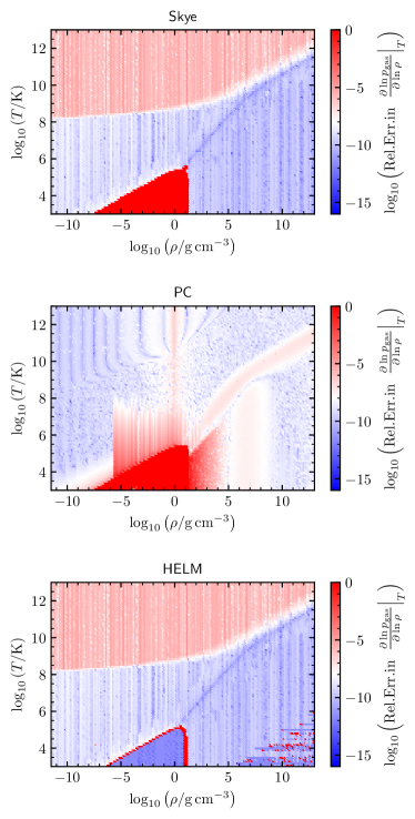
Figure 2: The logarithm of the relative difference between $\partial\ln p_{\rm gas}/\partial\ln\rho|_{T}$ and a finite difference approximation to the same is shown as a function of $T$ and $\rho$ for each of Skye, PC, and HELM for an equal-mass fraction mixture of ${}^{12}\mathrm{C}$ and ${}^{16}\mathrm{O}$. The feature in Skye and PC at intermediate densities and low temperatures results from negative pressures caused by the assumption of a fully ionized free energy in a region that should form bound states, indicating that these EOSes are not valid in that limit.

In general the quality of derivatives degrades as we look to higher orders because there is more room for precision issues. Figure 3 shows the relative difference between the reported derivative $\partial\chi_{T}/\partial\ln\rho|_{T}=\partial^{2}\ln p/\partial\ln\rho\,\partial\ln T$ and an iteratively acquired high-precision numerical derivative for Skye and HELM. Once more at high temperatures above $10^{9}\,\mathrm{K}$ the system becomes dominated by electron-positron pairs and so nearly independent of the $\rho$. The derivatives in Skye and HELM are then pushed towards the limits of floating point precision, degrading their quality.

$\partial\chi_{T}/\partial\ln\rho|_{T}$ is not reported natively by PC so we could not include PC in this comparison. Because MESA requires this derivative, when PC is used in MESA this derivative is estimated using finite differences in $\ln\rho$. This results in derivatives that are accurate at only around the $10^{-2}$ level, which was often a bottleneck in stellar evolution calculations.

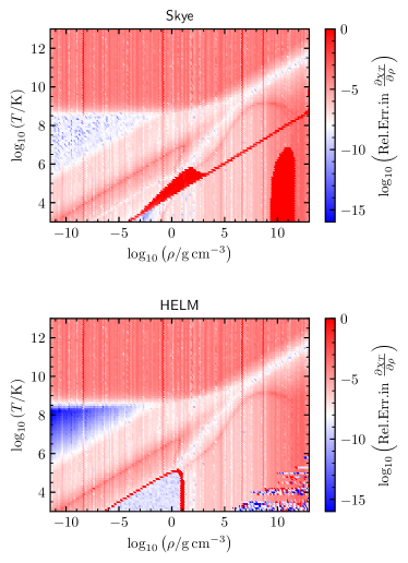
Figure 3: The logarithm of the relative difference between $\partial\chi_{T}/\partial\ln\rho|_{T}$ a finite difference approximation to the same is shown as a function of $T$ and $\rho$ for Skye and HELM for an equal-mass fraction mixture of ${}^{12}\mathrm{C}$ and ${}^{16}\mathrm{O}$.

6.2 Thermodynamic Consistency

The first law of thermodynamics is an exact differential and thus implies several consistency relations between the different thermodynamic quantities. These are (Timmes & Swesty, 2000; Paxton et al., 2019, see their Appendix A.1.3)

$$\mathrm{dpe}\equiv\frac{\rho^{2}}{p}\left.\frac{\partial e}{\partial\rho}\right|_{T,\{y_{j}\}}+\frac{T}{p}\left.\frac{\partial p}{\partial T}\right|_{\rho,\{y_{j}\}}-1 =0$$ (59)

$$\mathrm{dse}\equiv T\frac{\partial s/\partial T|_{\rho,\{y_{j}\}}}{\partial e/\partial T|_{\rho,\{y_{j}\}}}-1 =0$$ (60)

$$\mathrm{dsp}\equiv-\rho^{2}\frac{\partial s/\partial\rho|_{T,\{y_{j}\}}}{\partial p/\partial T|_{\rho,\{y_{j}\}}}-1 =0.$$ (61)

If these relations are not satisfied an equation of state is thermodynamically inconsistent. For simulations of physical scenarios this can result in artificial generation or loss of energy or entropy or incorrect conversion between these and mechanical work. Moreover thermodynamic inconsistency means that different forms of the same physical equations are not even mathematically identical. For instance, neglecting changes in composition, in stellar evolution the equation of local energy conservation is often written as (Paxton et al., 2015)

$$\frac{de}{dt}-\frac{p}{\rho}\frac{d\ln\rho}{dt}=T\frac{ds}{dt},$$ (62)

or alternatively as

$$c_{p}T\left[(1-\nabla_{\rm ad}\chi_{T})\frac{d\ln T}{dt}-\nabla_{\rm ad}\chi_{\rho}\frac{d\ln\rho}{dt}\right]=T\frac{ds}{dt}.$$ (63)

For numerical reasons it is often preferable to use one form over another, but these forms are only mathematically equivalent to the extent that the EOS is thermodynamically consistent.

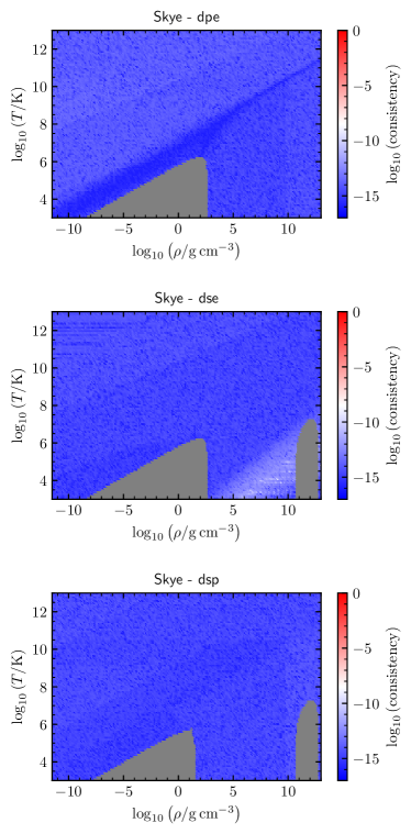
Figure 4: The thermodynamic consistency measures $\mathrm{dpe}$, $\mathrm{dse}$, and $\mathrm{dsp}$ are shown for Skye on a logarithmic scale for an equal-mass fraction mixture of ${}^{16}\mathrm{O}$ and ${}^{20}\mathrm{Ne}$. Grey indicates regions where the result is NaN due to negative reported entropy, energy, or pressure (solid regions) resulting in undefined logarithms in intermediate steps of the calculation. The feature at intermediate densities and low temperatures indicates negative pressures caused by our assumption of a fully ionized free energy in a region that should form bound states, indicating that Skye is not valid in that limit.

Figure 4 shows the quantities $\mathrm{dpe}$, $\mathrm{dse}$, and $\mathrm{dsp}$ from Skye as functions of $\rho$ and $T$ for an equal-mass fraction mixture of ${}^{16}\mathrm{O}$ and ${}^{20}\mathrm{Ne}$. Because Skye is derived from a free energy formalism it is thermodynamically consistent to the limits of floating-point precision.

Note that this high degree of consistency should not be confused with physical accuracy. Skye returns numerically accurate partial derivatives and thermodynamically consistent quantities, but this is not the same as physical accuracy, which is a matter of how well the input physics matches Nature.

6.3 Crystallization Curves

We demonstrate where and how crystallization occurs in Skye by first considering a pure ${}^{12}\rm C$ plasma at $\rho=10^{7}\mathrm{g\,cm^{-3}}$. Figure 5 shows the location of crystallization and how that depends on which terms are included in the free energy. The dotted line shows the result of considering only the classical OCP free energy, which we achieve by artificially forcing $\eta\to 0$ and deactivating the screening terms. This illustrates that crystallization is centered at the established value of $\Gamma\approx 175$ (e.g., Potekhin & Chabrier, 2000, and references therein) and occurs over an an interval of width $\Delta\Gamma\approx 10$ due to the blur described in Section 3. Including quantum corrections causes a small shift ($\delta\Gamma\lesssim 1$) to higher values of $\Gamma$. Adding screening results in much larger shift ($\delta\Gamma\approx 7$) towards lower values of $\Gamma$.

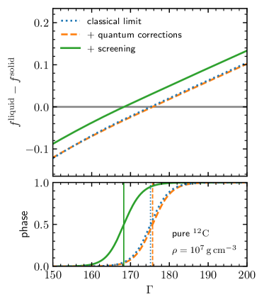
Figure 5: The liquid-solid free energy difference (top panel) and phase $\phi$ (bottom panel) as a function of $\Gamma$ for pure ${}^{12}\rm C$ plasma at $\rho=10^{7}\mathrm{g\,cm^{-3}}$. We show the effects of different terms in the free energy by first showing the result in the classical limit (forcing $\eta\to 0$), then adding quantum effects, and finally including screening corrections.

Skye determines the phase (solid/crystalline or liquid) self-consistently via free energy minimization, so it can model the effects of varying composition on melting temperature. Figure 6 shows the phase as a function of temperature and composition in a ${}^{12}{\rm C}$-${}^{16}{\rm O}$ mixture. The x-axis, $x_{\rm O}$, is the ${}^{16}\rm O$ number fraction. The y-axis, $T/T_{\rm m,C}$, is the ratio of the temperature to the melting temperature of a pure ${}^{12}\rm C$ plasma. Because $\phi$ is a smoothed measure of the phase it takes a non-zero width to transition from $\phi\approx 0$ to $\phi\approx 1$.

The work of Blouin et al. (2020), which adopts a Gibbs–Duhem integration technique coupled to Monte Carlo simulations, provides a useful point of comparison. Their phase curve is calculated at $P=10^{24}\,\mathrm{erg\,cm^{-3}}$ and so we calculate the Skye phase at $\rho=10^{7}\,\mathrm{g\,cm^{-3}}$ which corresponds to a similar pressure of $P\approx 8\times 10^{23}\,\mathrm{erg\,cm^{-3}}$. In Figure 6, we show the Blouin et al. (2020) liquidus and solidus. The reference melting temperature used for the Blouin et al. (2020) liquidus and solidus curves is the $T_{\rm m,C}$ value from Blouin et al. (2020), which differs from the Skye value. Recall Skye does not consider phase separation, so it produces a single (blurred) transition line.

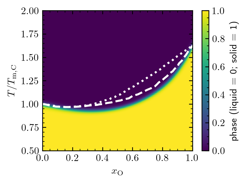
Figure 6: The phase $\phi$ as a function of the ratio of the temperature to the melting temperature of a pure ${}^{12}\rm C$ plasma, $T/T_{\rm m,C}$, and ${}^{16}\rm O$ number fraction, $x_{\rm O}$, at fixed density $\rho=10^{7}\mathrm{g\,cm^{-3}}$ for a mixture of ${}^{12}\rm C$ and ${}^{16}\rm O$. The white lines are the liquidus (dotted) and solidus (dashed) from Blouin et al. (2020).

As an example of how simple it is to swap out individual components in the Skye framework, Figure 7 shows the result when we replace the (default) fit of Potekhin & Chabrier (2013) for the solid mixing corrections with the form proposed by Ogata et al. (1993). The Potekhin & Chabrier (2013) form is in part motivated to overcome unphysical behavior present in the Ogata et al. (1993) fit at charge ratios $R>2$, though a C/O mixture ($R=4/3$) is not in the troublesome regime.

The agreement shown in Figure 7 between Blouin et al. (2020) and Skye when using Ogata et al. (1993) is anticipated. The results of Blouin et al. (2020) agree well with the results of Medin & Cumming (2010). In turn, Skye resembles the analytic-fit-based approach of Medin & Cumming (2010), with the same extension from two-component to multi-component plasmas, and Medin & Cumming (2010) uses the Ogata et al. (1993) formulation of the solid mixing free energy.

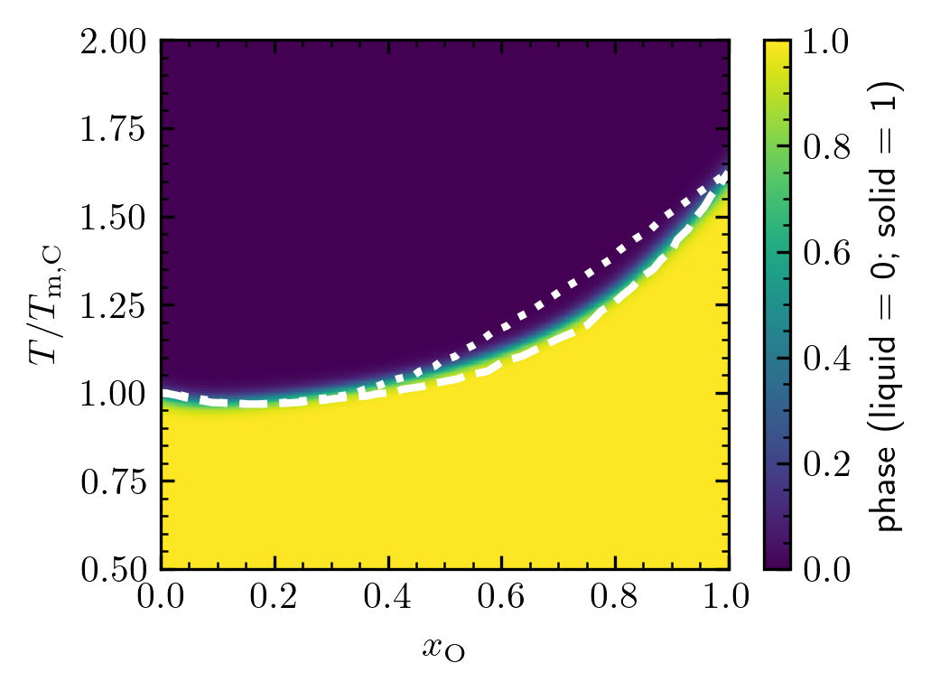
Figure 7: Same as Figure 6, except replacing the default solid mixing free energy from Potekhin & Chabrier (2013) with the form proposed by Ogata et al. (1993).

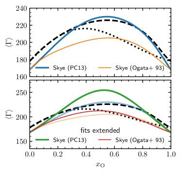
Figure 8: Value of $\langle\Gamma\rangle$ corresponding to the center of the Skye phase transition ($\phi=0.5$) as function of ${}^{16}\rm O$ number fraction $x_{\rm O}$ at fixed density $\rho=10^{7}\,\mathrm{g\,cm^{-3}}$ for a mixture of ${}^{12}\rm C$ and ${}^{16}\rm O$. The top panel compares the Skye results using the indicated solid mixing correction. The bottom panel shows the results when extending the limits of the solid and liquid fits (see text). The curves from the top panel are faintly shown for ease of comparison. In both panels, the black lines are the liquidus (dotted) and solidus (dashed) from Blouin et al. (2020).

.

The results shown in Figures 6 and 7 are summarized in the top panel of Figure 8 which plots the value of the average Coulomb parameter $\langle\Gamma\rangle$ at crystallization (defined as when $\phi=0.5$) as a function of the ${}^{16}\rm O$ number fraction. For pure compositions, the Skye phase transition occurs at a $\langle\Gamma\rangle$ value of about 10 less than Blouin et al. (2020), primarily reflecting the screening corrections shown in Figure 5. The two approaches to the mixing corrections give significantly different values for the phase transition in an equal (by number) mixture, with the Ogata et al. (1993) form yielding $\langle\Gamma\rangle\approx 205$ and the Potekhin & Chabrier (2013) form yielding $\langle\Gamma\rangle\approx 230$, with the Blouin et al. (2020) results intermediate.

Because the range of $\Gamma_{j}$ where both the liquid and solid free energy fits are valid is small, for charge ratios greater than $(\Gamma_{\rm max}^{\rm liquid}/\Gamma_{\rm min}^{\rm solid})^{1/2}\approx 1.1$ one species or the other will typically be extrapolated at the phase transition. To illustrate this effect, the bottom panel of Figure 8 shows a ‘fits extended’ calculation where we used $\Gamma_{\rm min}^{\rm solid}=100$ and $\Gamma_{\rm max}^{\rm liquid}=300$. This shows that the transition $\langle\Gamma\rangle$ may depend at the 10 per-cent level on the choice of $\Gamma_{\rm max}^{\rm liquid}$ and $\Gamma_{\rm min}^{\rm solid}$.

The structure of Skye demands individual fits that behave well over wide parameter ranges and a set of prescriptions that can collectively work well together. This is especially necessary for determining the location of the phase transition, given the small relative difference between the liquid and solid free energies. We observe that Skye, at some unusual conditions, reports that material returns to the liquid state at sufficiently low temperature as a result of the quantum corrections. We discuss this behavior in Appendix D. We hope that the ease of experimentation with Skye can help motivate improved fits for some of the key quantities.

6.4 Comparison with Other EOS

We now compare various outputs from Skye, PC and HELM. Figure 9 shows the adiabatic index $\Gamma_{1}$ as a function of $\rho$ and $T$ for an equal-mass fraction mixture of ${}^{12}\mathrm{C}$ and ${}^{16}\mathrm{O}$. The upper panel is for Skye  the others show the signed logarithm of the relative difference between Skye and PC and HELM. The outlined contour shows where $\Gamma_{1}=4/3$, signalling onset of the pair production instability.

At high temperatures and low densities ($T/10^{4}\,\mathrm{K}>(\rho/10^{-10}\,\mathrm{g\,cm^{-3}})^{1/3}$), Skye and HELM agree to better than one part in $10^{5}$, and both differ from PC by including positrons, which produce the feature that runs across the figure near $10^{9}\,\mathrm{K}$.

At lower temperatures and higher densities Skye and PC generally agree to better than one part in $10^{3}$. The first exception is at intermediate densities and low temperatures, where both Skye and PC show artifacts caused by the assumption of a fully ionized free energy in a region that should form bound states, indicating these equations of state are not valid in that limit. The other major difference is a series of scars at extreme densities and very low temperatures, which Skye inherits from the ideal electron-positron term in HELM. In that regime computing thermodynamic quantities often requires subtracting very similar numbers, resulting in loss of precision. The analytic fits PC uses for the ideal electron gas avoid this issue and produce smooth results there.

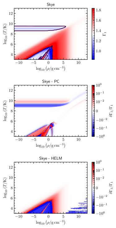
Figure 9: The adiabatic index $\Gamma_{1}$ is shown as a function of temperature and density for each of Skye, PC, and HELM for an equal-mass fraction mixture of ${}^{12}\mathrm{C}$ and ${}^{16}\mathrm{O}$. The upper panel is for Skye  the others show the relative difference between Skye and PC and HELM. The outlined contour shows where $\Gamma_{1}=4/3$, signalling onset of the pair production instability. Note that the outlined region in the bottom-right has $\Gamma_{1}<4/3$ because of precision issues in the ideal electron-positron tables and is not a sign of a physical instability.

Closely related to $\Gamma_{1}$, and of particular interest for asteroseismology, is the adiabatic temperature gradient $\nabla_{\rm ad}$. Figure 10 shows $\nabla_{\rm ad}$ as a function of $\rho$ and $T$ for the same composition used in Figure 9. Once more at high temperatures Skye and HELM agree at the $10^{-5}$ level, and both differ from PC by including positrons. At lower temperatures we see an order-unity difference between Skye and PC which stretches along a line of nearly constant $\langle\Gamma\rangle$. This difference is because PC places the phase transition at a fixed location in $\langle\Gamma\rangle$ while Skye determines the phase boundary from the input physics, which in this instance causes it to place the boundary at a slightly different $\langle\Gamma\rangle$. The other major difference is that Skye again shows scars at very high density that come from loss of precision in the ideal electron-positron term in HELM. Other than that region Skye and PC generally agree to better than one percent.

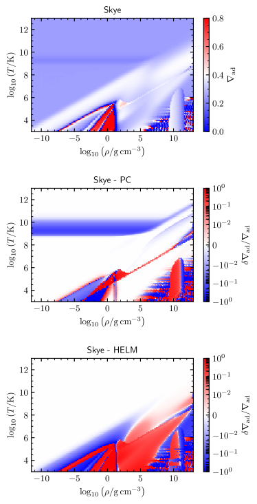
Figure 10: The adiabatic temperature gradient $\nabla_{\rm ad}$ is shown as a function of temperature and density for each of Skye, PC, and HELM for an equal-mass fraction mixture of ${}^{12}\mathrm{C}$ and ${}^{16}\mathrm{O}$. The upper panel is for Skye  the others show the relative difference between Skye and PC and HELM.

One of the most important quantities for white dwarf cooling models (Section 6.5) is the specific heat. Figure 11 compares this quantity between PC and Skye for ${}^{4}\rm He$ and ${}^{12}\rm C$. In the case of ${}^{12}\rm C$, the agreement is generally good, with some disagreement at the $\approx 10\%$ level around the temperature of crystallization in the highest density line shown. The dips near the location of the Skye phase transition are due to thermodynamic extrapolation and will be discussed in detail in Section 6.5.

In the case of ${}^{4}\rm He$, in coolest parts of the liquid regime, PC produces specific heats that fall rapidly with decreasing temperature and even become negative. This reflects a difference in the assumed physics. This version of PC contains only the leading-order term in the Wigner-Kirkwood expansion (which is pushed beyond its range of validity of $\eta_{j}\lesssim 1$ in these plots), while Skye includes the prescription of Baiko & Yakovlev (2019) which is valid up to $\eta_{j}\approx 12$. At densities $\log_{10}(\rho/{\rm g\,cm^{-3}})=$ 4, 5, and 6, Figure 11 illustrates that the Baiko & Yakovlev (2019) prescription reasonably joins onto the $\propto T^{3}$ specific heat of the Debye regime. For higher ${}^{4}\rm He$ densities, this join becomes less smooth and by $\log_{10}(\rho/{\rm g\,cm^{-3}})=7$, Skye too develops regions of negative specific heat, because by $\rho\gtrsim 10^{7}\mathrm{g\,cm^{-3}}$ for Helium, $r_{s,j}\lesssim 300$ which is beyond the validity of the fit by Baiko & Yakovlev (2019). Eliminating these features awaits future improvements in prescriptions for the free energy of the quantum Coulomb liquid.

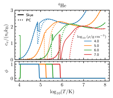
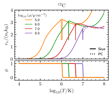
Figure 11: Comparison of specific heat between Skye and PC for ${}^{4}\rm He$ (top plot) and ${}^{12}\rm C$ (bottom plot) as function of temperature at an indicated set of densities. Within each plot, the top panel shows the total specific heat at constant volume per ion for each of Skye and PC, while the bottom panel shows the Skye phase.

6.5 White Dwarf Cooling Curves

We have computed white dwarf (WD) cooling curves using the Modules for Experiments in Stellar Astrophysics (MESA; Paxton et al., 2011, 2013, 2015, 2018, 2019) software instrument. MESA uses a blend of several equations of state, and we have configured the blend to use Skye in regions of high density or temperature. Details of MESA, the blend, and other microphysics inputs are provided in Appendix A.

Our example WD model is 0.6 $M_{\odot}$ with a C/O core and an initial hydrogen layer mass of $5\times 10^{-5}\ M_{\odot}$. This model is based on the MESA test case wd_cool_0.6M from MESA release version 15140. Our cooling tracks begin when the model has a core temperature of $\log_{10}(T_{\rm c}/K)=7.8$ and luminosity of 1 $L_{\odot}$, and the WD cools until the core temperature reaches $\log_{10}(T_{\rm c}/K)=6.0$. We use the DA WD atmosphere tables of Rohrmann et al. (2012) as our outer boundary conditions for these WD cooling models. The prior evolution of the WD progenitor model included heavy element sedimentation so that the envelope is stratified and the outer layers are composed of pure hydrogen, but for simplicity we turn diffusion off for the cooling tracks calculated in this paper. These models therefore do not include any cooling delay associated with heating from sedimentation of ²²Ne such as that described in Paxton et al. (2018) and Bauer et al. (2020). Instead, we focus on cooling effects directly associated with EOS quantities such as heat capacity and latent heat released by crystallization.

We run several versions of the WD cooling model described above, using either Skye or the PC EOS in the high density regime ($\log_{10}(\rho/{\rm g\,cm^{-3}})>4$). The PC EOS provides thermodynamics for both liquid and solid states, with the location of the phase transition a free parameter to be set by the user. As a baseline model for comparison, we run the cooling WD with crystallization in PC set to occur when the plasma reaches $\langle\Gamma\rangle=230$, but with no latent heat included in the model. Previous WD cooling models using MESA have adopted this choice of $\langle\Gamma\rangle=230$ as a rough approximation of the C/O phase curve in mixtures relevant for WD interiors (see Bauer et al. (2020) for a recent example and further discussion). We also run the WD cooling model using PC with crystallization occurring at $\langle\Gamma\rangle=175$ and $\langle\Gamma\rangle=230$ with the latent heat included in the models. When running with the PC EOS, MESA models include the latent heat by taking the difference of entropy $s$ in the solid and liquid states, smoothed over a narrow range of $\Gamma$ around the phase transition (e.g. in our case $228<\Gamma<232$ for crystallization at $\langle\Gamma\rangle=230$). The latent heating term is then constructed as $\epsilon_{\rm latent}=-T(s_{\rm solid}-s_{\rm liquid})/\delta t$, where $\delta t$ is the timestep. This latent heat is included in the evolution as part of $\epsilon_{\rm grav}\equiv-Tds/dt$ (Paxton et al., 2018). Finally, we run the same WD cooling model with Skye as the EOS, which includes the phase transition and the latent heat according the phase curves shown in Figures 6 and 8.

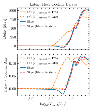
Figure 12: Comparison of latent heat cooling delays for Skye and PC with crystallization occurring at two different values of $\langle\Gamma\rangle$. All delays are relative to a model run using the PC EOS with $\langle\Gamma\rangle_{\rm crystal}=230$ and no latent heat release.

Figure 12 shows the cooling delay introduced into WD models by latent heat from crystallization in models run with each of the PC EOS and Skye. For Skye we performed two sets of calculations, one with the default extrapolation settings and another ‘fits extended’ calculation where we used $\Gamma_{\rm min}^{\rm solid}=100$ and $\Gamma_{\rm max}^{\rm liquid}=300$.

In general the Skye models agree well with the PC model run with crystallization occurring at $\langle\Gamma\rangle=230$, which represents the previous state of the art for WD cooling in MESA. Before crystallization begins around $\log_{10}(L/L_{\odot})=-3.8$, the lower panel of Figure 12 also shows that the Skye WD models agree with the overall cooling age of the PC model to better than 1%.

The Skye models also agree well with each other despite the ‘fits extended’ version applying the free energy fits over a wider range of temperatures. The reason for this is that Skye is thermodynamically consistent, so the overall cooling delay produced by the phase transition is insensitive to the choice of $\Gamma_{\rm max}^{\rm liquid}$ and $\Gamma_{\rm min}^{\rm solid}$. To see this note that the entropy deep in the liquid phase (all $\Gamma_{j}<\Gamma_{\rm max}^{\rm liquid}$) is independent of the extrapolation process, and likewise for the entropy deep in the solid phase (all $\Gamma_{j}>\Gamma_{\rm min}^{\rm solid}$). Hence, if the temperature varies little across the transition and extrapolation window then $\int T\partial s/\partial TdT$, counting the $\epsilon_{\rm latent}$ term, is nearly independent of the extrapolation limits.

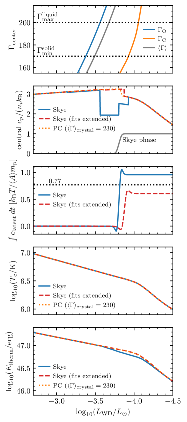
Figure 13: Core thermodynamic properties as a function of luminosity for WD cooling models running on Skye and PC. In the second panel Skye phase refers to the quantity $\phi$ from equation (42).

Figure 13 gives a comparison of the interior properties of the WD cooling models from Skye and PC with crystallization at $\langle\Gamma\rangle=230$. As expected, the $L$–$T_{\rm c}$ relation agrees very well between Skye and PC models, reflecting the similar input physics underlying these two EOSs. Similarly, the total WD thermal content, defined as $E_{\rm therm}\equiv\int c_{p}T\,dm$, agrees very well between the two models.

The heat capacity $c_{p}$ in Figure 13 shows some disagreement in the region near the phase transition from liquid to solid. The notch-like behavior in the Skye $c_{p}$ is a result of our thermodynamic extrapolation prescription (Section 2.3). This is because the one-component plasma contribution to $\partial s/\partial T$ vanishes when we extrapolate, so the contribution to $c_{v}$ vanishes:

$$c_{v} =\left.\frac{\partial e}{\partial T}\right|_{\rho}$$

$$=\left.\frac{\partial(F+Ts)}{\partial T}\right|_{\rho}$$

$$=\left.\frac{\partial F}{\partial T}\right|_{\rho}+s+T\left.\frac{\partial s}{\partial T}\right|_{\rho}$$

$$=T\left.\frac{\partial s}{\partial T}\right|_{\rho}.$$ (64)

Therefore, for any species at a $\Gamma_{j}$ where its free energy is being extrapolated, its OCP contribution to $c_{v}$ vanishes. Because $c_{p}\sim c_{v}$, this causes a drop in $c_{p}$ as well. Reading from left to right in the $c_{p}$ panel of Figure 13, the core begins in the liquid phase and initially no extrapolation is needed for the liquid phase free energy because $\Gamma_{j}<\Gamma_{\rm max}^{\rm liquid}$ for all species. As the core cools, the $\Gamma_{j}$ rise. The heat capacity falls sharply when $\Gamma_{{}^{16}\rm O}$ reaches $\Gamma_{\rm max}^{\rm liquid}$ because past that point we extrapolate the OCP free energy of ${}^{16}\rm O$. The core continues cooling and then crystallizes at $\log L/L_{\odot}=-3.8$. At this point the heat capacity is determined by the solid phase free energy. Because $\Gamma_{{}^{16}\rm O}>\Gamma_{\rm min}^{\rm solid}$, the OCP free energy of ${}^{16}\rm O$ is no longer extrapolated, but $\Gamma_{{}^{12}\rm C}<\Gamma_{\rm min}^{\rm solid}$ so the free energy of ${}^{12}\rm C$ is now extrapolated in the solid phase. Finally, once $\log L/L_{\odot}=-3.9$, $\Gamma_{{}^{12}\rm C}>\Gamma_{\rm min}^{\rm solid}$ so we stop extrapolating the ${}^{12}\rm C$ free energy, causing a jump in $c_{p}$. At this stage no species are extrapolated, and the heat capacity remains smooth for the rest of the run.

As before we note that because Skye is thermodynamically consistent the overall cooling delay is insensitive to the choice of limits for thermodynamic extrapolation and hence to these features in $c_{p}$. So for instance in Figure 13 extrapolation reduces $c_{p}$ near the phase transition relative to the ‘fits extended’ version of Skye. The third panel of Figure 13 shows the total latent heat released in the core in terms of the thermal energy per ion at the temperature of crystallization, and we see that this is decreased for the ‘fits extended’ version. Thus the decrease in $c_{p}$ is offset in the overall cooling calculating by an increase in $\epsilon_{\rm latent}$, resulting in the regular and ‘fits extended’ versions of Skye showing very similar cooling curves in Figure 12.

In both the regular and ‘fits extended’ versions of Skye we see that the overall magnitude of the latent heat is similar to the value of $0.77k_{\rm B}T/\langle A\rangle m_{\rm p}$ calculated by Salaris et al. (2000), which has often been adopted in recent studies of WD cooling using other stellar evolution codes (e.g., Camisassa et al. 2019). It is likewise similar to the results of Potekhin & Chabrier (2013), who obtained an improved value of $0.75k_{\mathrm{B}}T/Am_{\mathrm{p}}$ in the case of the one component plasma with the ‘rigid’ electron backgroung and showed that the allowance for electron polarization/screening can lead to deviations of up to a factor of two from this value.

In our testing these sharp features in $c_{p}$ have not caused any convergence problems in MESA. However, if this behavior is undesirable, $\Gamma_{\rm min}^{\rm solid}$ can be lowered and $\Gamma_{\rm max}^{\rm liquid}$ can be raised to ensure that, for any given composition, extrapolation is only used for the liquid phase when the system is solid, and vice versa, with the caveat that this risks using fitting formulas beyond the region in which they are known to be accurate. This is what is shown in the ‘fits extended’ curves in Figures 12 and 13, where we used $\Gamma_{\rm min}^{\rm solid}=100$ and $\Gamma_{\rm max}^{\rm liquid}=300$. Our hope is that future work on multi-component plasmas will provide a way to capture the behavior of, e.g., low-$\Gamma$ carbon in a multi-component solid. This could take the form of e.g., fits for the two-component plasma free energy at the phase transition as a function of the charge ratio between the two species.

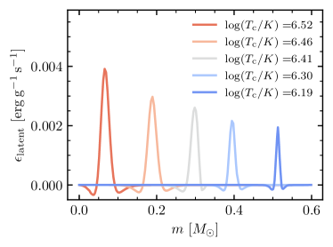
Figure 14: Evolution of the latent heating term from Skye as the WD model cools and the crystallization front moves from the center toward the surface.

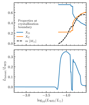
Figure 15: Upper panel: Curves showing the mass coordinate and composition of material at the crystallization boundary as a function of WD luminosity. Lower panel: Total luminosity from latent heating as a fraction of the WD luminosity, where $L_{\rm latent}\equiv\int\epsilon_{\rm latent}\,dm$.

Figures 14 and 15 show more details about the latent heating term from Skye in our WD cooling model. Figure 14 shows how the blurred phase transition distributes the latent heat in the WD interior as the crystallization front moves outward while the WD cools. Integrating these heating profiles over the entire WD gives a total latent heating luminosity $L_{\rm latent}$, which is shown in Figure 15. The upper panel of that figure also shows the composition and mass coordinate location of the crystallization boundary (defined as the location where Skye phase = 0.5). We note that as the crystallization front moves outward, there is a brief pause in crystallization and the latent heating goes to zero when the front reaches a location where the core composition becomes more carbon-rich. This location corresponds to the outer edge of the former convective He-burning core at the end of central He-burning, where C/O layers exterior to this point were produced by subsequent He shell burning and therefore have a different C/O composition than the interior homogeneous core. This relatively carbon-rich layer has a lower crystallization temperature than the adjacent C/O core interior to it, and so the core temperature must cool further before crystallization resumes and the latent heat returns.

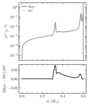
Figure 16: Upper panel: The Brünt-Väisälä frequency is shown as a function of mass coordinate for the Skye and PC WD models at a time when $\log T_{\rm c}/\mathrm{K}=7.05$ and $T_{\rm eff}=11,800\,\mathrm{K}$. Lower panel: The relative difference between the two models is shown as a function of mass coordinate.

Finally, Figure 16 shows the profile of the Brünt-Väisälä frequency for both the Skye and PC WD models, as well as the relative difference between the two. The differences are generally of order a few percent. For $m>0.3M_{\odot}$, there are differences in the composition gradient region. These arise because Skye treats the density $\rho$ as the baryonic mass density whereas PC treats it as the physical mass density. Either choice is valid, but neither is fully consistent with how MESA computes either the Brünt-Väisälä frequency or hydrostatic equilibrium, and these inconsistencies produce the differences we see for $m>0.3M_{\odot}$.

7 Execution Efficiency

Skye is designed to be fast enough to evaluate at runtime in stellar evolution calculations. We benchmarked Skye, HELM, and PC on a single core of an Intel Core i9 (I9-9980HK) CPU running at 2.4GHz. For this test PC was modified to use CR-LIBM for mathematical operations to ensure bit-for-bit identical results across platforms just like Skye and HELM.

We evaluated each EOS on a log-spaced grid in $\rho$ spanning $10^{-10}-10^{10}\,\mathrm{g\,cm^{-3}}$ with 600 points and in $T$ spanning $10^{3}-10^{10}\,\mathrm{K}$, with 500 points. We require each EOS to return all of the quantities listed in Section 3 except for the Skye-specific ones, as well as the partial derivatives of each of those quantities with respect to $\rho$ and $T$. Because PC does not natively provide those derivatives, we use three calls of PC per point and then extract the additional derivatives with finite differences.

Averaged over all points in our grid, Skye takes $17\mu\mathrm{s}$ per call, PC takes $9\mu\mathrm{s}$ per call, and HELM takes $6\mu\mathrm{s}$ per call, where again we evaluate PC three times per call to produce the additional derivatives required by stellar evolution software instruments such as MESA.

As a second benchmark, we tracked the time spent in the MESA EOS module during the white dwarf cooling study from Section 6.5. The EOS accounted for 10.5 per-cent of total run time when using PC, and 13.9 per-cent of total run time when using Skye. This understates the difference between the two slightly because some of the time the stellar model is at a temperature and density where neither PC nor Skye are used, but shows that the runtime difference is minimal not only on a grid but also in practice in stellar evolution calculations.

Skye and PC have similar performance for several reasons:

1. The physics that enters these equations of state is similar.

2. Our automatic differentiation type is heavily optimized, and in many cases produces performance similar to hand-coded derivatives.

3. The additional cost of determining higher-order derivatives with automatic differentiation happens to be very similar to the overhead of calling PC three times to obtain the same derivatives with finite differences.

4. While Skye has to compute the non-ideal free energy twice to obtain phase information, this extra cost relative to PC is offset by the fact that Skye uses free energy tables for the ideal electron-positron contribution while PC computes this with more expensive fitting formulas.

We determined (3) by producing a modified version of PC which produces higher-order derivatives using automatic differentiation rather than finite differences and found its performance to be similar to the unmodified PC.

HELM is much faster than either Skye or PC for three main reasons. First, HELM uses an average composition characterized by the mean molecular weight and mean charge, rather than directly using the full composition vector $\{y_{j}\}$. Second, the computationally expensive parts of HELM (a root-find for the electron chemical potential, high precision Fermi-Diac integrals, and nearly all operations involving division, exponentials, and power functions) are tabulated on a logically rectalinear array. Each call to HELM then consists of hash table lookups followed by calls to fast polynomial interpolation functions. Third, thermodynamic information for neighboring points are located next to each other in physical memory. Ordered sweeps, such as from the surface of a stellar model to the center, will usually access data already loaded into the processor cache rather than having to access data from the slower main memory. This reduction in the time required to access information from memory boosts the execution efficiency.

8 Availability

Skye is distributed as part of the eos module of the MESA stellar evolution software instrument. It is also available as a standalone package from https://github.com/adamjermyn/Skye, and the version used here is available from Jermyn et al. (2021a). Compilation is supported on the GNU Fortran compiler version 10.2.0.

9 Future Work

Because Skye is a framework for developing new EOS physics we expect future work to bring several key improvements. First, and most pressing, is handling of partial ionization and neutral matter. With that Skye could be used across the entire range of densities and temperatures which arise in stellar evolution calculations. This could be done in a Debye-Huckle-Thomas-Fermi formalism (Cowan & Kirkwood, 1958) or other approaches in the physical picture (Rogers & Nayfonov, 2002), or else via free energy minimization (Irwin, 2004) in the chemical picture (Saumon et al., 1995). The key constraint in each of these approaches is that Skye needs to remain fast enough to use in practical stellar evolution calculations. Our hope is that the flexibility afforded to Skye by its automatic differentiation machinery will allow us to rapidly prototype and test these various possibilities.

Along similar lines, Skye could be made to support phase separation by minimizing the free energy with respect to the compositions of the liquid and solid phases. The major bottleneck to supporting this is the current lack of Fortran compiler support for parameterized derived types. Once this compiler challenge is resolved, phase separation physics should not be difficult to implement.

More broadly, we make Skye openly available with the hope that it will grow into a community resource to use automatic differentiation to explore analytic free energy terms that captures improvements in existing physics and development of new or not yet considered physics.

Appendix A MESA

Our calculations of stellar structure and evolution were performed with commit 21fd6fa of the MESA software instrument, based upon the recent release r15140. We patched this commit to use the version of PC which ships with MESA revision 12778 because that is more similar to the original PC EOS. MESA uses a blend of Skye, OPAL (Rogers & Nayfonov, 2002), SCVH (Saumon et al., 1995), FreeEOS (Irwin, 2004), and HELM Timmes & Swesty (2000). The blend uses Skye in most of the region where $T>10^{6.2}\,\mathrm{K}$ or $\rho>10^{4}\,\mathrm{g\,cm^{-3}}$, though the precise shape of the blend between this EOS and the others is more complicated than a simple cutoff (see Figure 17), and was determined to minimize the the difference in energy between equations of state across the blend.

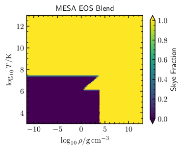
Figure 17: The fraction of Skye used in the MESA EOS is shown as a function of density and temperature.

Radiative opacities are primarily from OPAL (Iglesias & Rogers, 1993, 1996), with low-temperature data from Ferguson et al. (2005) and the high-temperature, Compton-scattering dominated regime by Poutanen (2017). Electron conduction opacities are from Cassisi et al. (2007).

Nuclear reaction rates are a combination of rates from NACRE (Angulo et al., 1999), JINA REACLIB (Cyburt et al., 2010), plus additional tabulated weak reaction rates Fuller et al. (1985); Oda et al. (1994); Langanke & Martínez-Pinedo (2000). Screening is included via the prescription of Chugunov et al. (2007). Thermal neutrino loss rates are from Itoh et al. (1996).

Appendix B EOS Comparisons

For standalone EOS comparisons we use the version of PC which ships with MESA revision 12778, which notably smooths thermodynamic quantities across the phase transition. This was a modification made for numerical reasons in MESA, but should not substantially affect the substance of our comparisons. We disable Coulomb corrections in HELM and enforce full ionization across the $\rho-T$ plane. We use the tabulated free energy for all HELM quantities, including $\partial p/\partial\rho|_{T}$ and $\partial^{2}p/\partial\rho^{2}|_{T}$, rather than the auxiliary tables which provide these separately. High quality numerical derivatives were determined using the $\mathrm{dfridr}$ option in the $\mathrm{eos\_plotter}$ routine in MESA.

Appendix C Data Availability

The data and related scripts used in this work are available at Jermyn et al. (2021b).

Appendix D Phase Transitions and Quantum Corrections

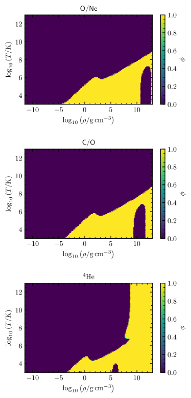
Figure 18: The phase $\phi$ is shown as a function of temperature and density for (upper) an equal-mass mixture of ${}^{16}\rm O$ and ${}^{20}\rm Ne$, (middle) an equal-mass mixture of ${}^{12}\rm C$ and ${}^{16}\rm O$, and (lower) pure ${}^{4}\rm He$.

Figure 18 shows the Skye phase $\phi$ as a function of $\rho$ and $T$ for three different compositions. At high temperatures and low densities the system is a liquid, and it crystallizes in the opposite limit. This standard OCP-like phase transition that occurs at approximately constant $\langle\Gamma\rangle$ is discussed in the main text. However, Figure 18 displays additional structure in the phase, which we determined to be primarily related to the quantum correction terms in the free energy. These features likely reflect limitations in the assumed prescriptions.

At high densities for the lightest elements ($\mathrm{H}$ and $\mathrm{He}$), quantum corrections dominate and favor the solid phase up to high temperatures. While a self-consistent consequence of the adopted inputs, we suspect this feature is spurious. However, as ${}^{4}\mathrm{He}$ and ${}^{1}\mathrm{H}$ are likely to have fused into heavier elements long before reaching these densities in typical astrophysical applications, we have done nothing to suppress this solidification in Skye.

At high densities and at low temperatures, quantum corrections dominate and cause the system to melt. This occurs at lower densities and temperatures for lower-mass lower-charge species: $10^{10}\,\mathrm{g\,cm^{-3}}$ for O/Ne, $10^{8}\,\mathrm{g\,cm^{-3}}$ for C/O, and $10^{4}\,\mathrm{g\,cm^{-3}}$ for ${}^{4}\mathrm{He}$). A similar effect has been seen in Monte Carlo calculations and analytic calculations (Chabrier, 1993; Ceperley, 1978; Jones & Ceperley, 1996). In those studies the Lindemann criterion was used to compute the quantum melt line, but the result has a rather different topology from the phase boundary we see (Figure 19). In particular we see the quantum melt only for a finite density range, whereas they predict it for all densities above a cutoff. The latter is more in line with our understanding of the physics of quantum melting, namely that it is driven by the zero-point energy of ions and so should only increase with increasing density. We therefore suspect that the topology of this melt region reflects limitations in our prescriptions for the OCP quantum corrections.

Moreover the temperature and density scale involved is rather different from Lindemann criterion calculations (Chabrier, 1993; Ceperley, 1978; Jones & Ceperley, 1996), though interestingly the scaling of these scales matches those from the Lindemann criterion. The melt line is predicted to peak around $k_{\rm B}T\approx 6\times 10^{-5}\,\mathrm{Ry}_{j}$, where

$$\mathrm{Ry}_{j}=(Z_{j}e)^{4}m_{j}/2\hbar^{2}$$ (D1)

is the ionic Rydberg. Instead we see a peak near $6\times 10^{-6}\,\mathrm{Ry}_{\rm ion}$. Likewise the melt line is predicted to peak in temperature when the dimensionless ion sphere radius

$$r_{s,j}\equiv\left(\frac{3m_{j}}{4\pi\rho}\right)^{1/3}\frac{m_{j}(Z_{j}e)^{2}}{\hbar^{2}}$$ (D2)

is of order $200$, and we see the peak around $1200$.

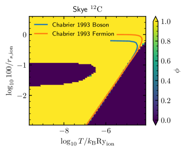
Figure 19: The phase $\phi$ is shown as a function of temperature in units of $\mathrm{Ry}_{\rm ion}$ and reciprocal ion spacing measured by $100/R_{S,\rm ion}$. The melt lines of Chabrier (1993) for bosons (blue) and fermions (orange) are over-plotted for comparison. This calculation was done for pure ${}^{12}\mathrm{C}$, but the choice of units means the results are universal for any pure ionic system.

Overall the disagreement between Skye and calculations based on the Lindemann criterion suggests caution in interpreting these results. This disagreement may be caused by our use of the fit by Baiko & Yakovlev (2019) beyond its range of validity, which is confined within the dark blue triangle at the lower right corner of Figure 19. These results are, however, a completely self-consistent consequence of the input physics so we have not done anything to impede quantum melting in Skye.

References

- Alastuey & Ballenegger (2012) Alastuey, A., & Ballenegger, V. 2012, Phys. Rev. E, 86, 066402, doi: 10.1103/PhysRevE.86.066402
- Alastuey et al. (2020) Alastuey, A., Ballenegger, V., & Wendland, D. 2020, Phys. Rev. E, 102, 023203, doi: 10.1103/PhysRevE.102.023203
- Angulo et al. (1999) Angulo, C., Arnould, M., Rayet, M., et al. 1999, Nuclear Physics A, 656, 3, doi: 10.1016/S0375-9474(99)00030-5
- Aparicio (1998) Aparicio, J. M. 1998, ApJS, 117, 627
- Baiko (2019) Baiko, D. A. 2019, MNRAS, 488, 5042, doi: 10.1093/mnras/stz2041
- Baiko et al. (2001) Baiko, D. A., Potekhin, A. Y., & Yakovlev, D. G. 2001, Phys. Rev. E, 64, 057402, doi: 10.1103/PhysRevE.64.057402
- Baiko & Yakovlev (2019) Baiko, D. A., & Yakovlev, D. G. 2019, MNRAS, 490, 5839, doi: 10.1093/mnras/stz3029
- Ballenegger et al. (2018) Ballenegger, V., Alastuey, A., & Wendland, D. 2018, Contributions to Plasma Physics, 58, 114, doi: 10.1002/ctpp.201700189
- Bartholomew-Biggs et al. (2000) Bartholomew-Biggs, M., Brown, S., Christianson, B., & Dixon, L. 2000, Journal of Computational and Applied Mathematics, 124, 171, doi: 10.1016/S0377-0427(00)00422-2
- Baturin et al. (2019) Baturin, V. A., Däppen, W., Oreshina, A. V., Ayukov, S. V., & Gorshkov, A. B. 2019, A&A, 626, A108, doi: 10.1051/0004-6361/201935669
- Bauer et al. (2020) Bauer, E. B., Schwab, J., Bildsten, L., & Cheng, S. 2020, ApJ, 902, 93, doi: 10.3847/1538-4357/abb5a5
- Becker et al. (2014) Becker, A., Lorenzen, W., Fortney, J. J., et al. 2014, ApJS, 215, 21, doi: 10.1088/0067-0049/215/2/21
- Blinnikov et al. (1996) Blinnikov, S. I., Dunina-Barkovskaya, N. V., & Nadyozhin, D. K. 1996, ApJS, 106, 171, doi: 10.1086/192334
- Blouin et al. (2020) Blouin, S., Daligault, J., Saumon, D., Bédard, A., & Brassard, P. 2020, A&A, 640, L11, doi: 10.1051/0004-6361/202038879
- Bludman & van Riper (1977) Bludman, S. A., & van Riper, K. A. 1977, ApJ, 212, 859, doi: 10.1086/155110
- Caillol (1999) Caillol, J. M. 1999, J. Chem. Phys., 111, 9695, doi: 10.1063/1.480302
- Camisassa et al. (2019) Camisassa, M. E., Althaus, L. G., Córsico, A. H., et al. 2019, A&A, 625, A87, doi: 10.1051/0004-6361/201833822
- Carr et al. (1961) Carr, W. J., Coldwell-Horsfall, R. A., & Fein, A. E. 1961, Physical Review, 124, 747, doi: 10.1103/PhysRev.124.747
- Cassisi et al. (2007) Cassisi, S., Potekhin, A. Y., Pietrinferni, A., Catelan, M., & Salaris, M. 2007, ApJ, 661, 1094, doi: 10.1086/516819
- Ceperley (1978) Ceperley, D. 1978, Phys. Rev. B, 18, 3126, doi: 10.1103/PhysRevB.18.3126
- Chabrier (1990) Chabrier, G. 1990, Journal de Physique, 51, 1607
- Chabrier (1993) —. 1993, ApJ, 414, 695, doi: 10.1086/173115
- Chabrier & Potekhin (1998) Chabrier, G., & Potekhin, A. Y. 1998, Phys. Rev. E, 58, 4941, doi: 10.1103/PhysRevE.58.4941
- Chugunov et al. (2007) Chugunov, A. I., DeWitt, H. E., & Yakovlev, D. G. 2007, Phys. Rev. D, 76, 025028, doi: 10.1103/PhysRevD.76.025028
- Cloutman (1989) Cloutman, L. D. 1989, ApJS, 71, 677, doi: 10.1086/191393
- Cowan & Kirkwood (1958) Cowan, R. D., & Kirkwood, J. G. 1958, Phys. Rev., 111, 1460, doi: 10.1103/PhysRev.111.1460
- Cox & Giuli (1968) Cox, J. P., & Giuli, R. T. 1968, Principles of stellar structure
- Cyburt et al. (2010) Cyburt, R. H., Amthor, A. M., Ferguson, R., et al. 2010, ApJS, 189, 240, doi: 10.1088/0067-0049/189/1/240
- Daeppen et al. (1990) Daeppen, W., Lebreton, Y., & Rogers, F. 1990, Sol. Phys., 128, 35, doi: 10.1007/BF00154145
- Däppen (2010) Däppen, W. 2010, Ap&SS, 328, 139, doi: 10.1007/s10509-010-0269-2
- Daramy-Loirat et al. (2006) Daramy-Loirat, C., Defour, D., de Dinechin, F., et al. 2006, CR-LIBM A library of correctly rounded elementary functions in double-precision, Research report, LIP,. https://hal-ens-lyon.archives-ouvertes.fr/ensl-01529804
- DeWitt & Slattery (1999) DeWitt, H., & Slattery, W. 1999, Contributions to Plasma Physics, 39, 97, doi: 10.1002/ctpp.2150390124
- DeWitt & Slattery (2003) —. 2003, Contributions to Plasma Physics, 43, 279, doi: 10.1002/ctpp.200310027
- Eggleton et al. (1973) Eggleton, P. P., Faulkner, J., & Flannery, B. P. 1973, A&A, 23, 325
- Farouki & Hamaguchi (1993) Farouki, R. T., & Hamaguchi, S. 1993, Phys. Rev. E, 47, 4330, doi: 10.1103/PhysRevE.47.4330
- Fattoyev et al. (2010) Fattoyev, F. J., Horowitz, C. J., Piekarewicz, J., & Shen, G. 2010, Phys. Rev. C, 82, 055803, doi: 10.1103/PhysRevC.82.055803
- Ferguson et al. (2005) Ferguson, J. W., Alexander, D. R., Allard, F., et al. 2005, ApJ, 623, 585, doi: 10.1086/428642
- Fuller et al. (1985) Fuller, G. M., Fowler, W. A., & Newman, M. J. 1985, ApJ, 293, 1, doi: 10.1086/163208
- Galam & Hansen (1976) Galam, S., & Hansen, J.-P. 1976, Phys. Rev. A, 14, 816, doi: 10.1103/PhysRevA.14.816
- Gong et al. (2001a) Gong, Z., Däppen, W., & Zejda, L. 2001a, ApJ, 546, 1178, doi: 10.1086/318307
- Gong et al. (2001b) Gong, Z., Zejda, L., Däppen, W., & Aparicio, J. M. 2001b, Computer Physics Communications, 136, 294
- Hansen & Vieillefosse (1975) Hansen, J., & Vieillefosse, P. 1975, Physics Letters A, 53, 187 , doi: https://doi.org/10.1016/0375-9601(75)90523-X
- Hempel et al. (2012) Hempel, M., Fischer, T., Schaffner-Bielich, J., & Liebendörfer, M. 2012, ApJ, 748, 70, doi: 10.1088/0004-637X/748/1/70
- Hunter (2007) Hunter, J. D. 2007, Computing In Science & Engineering, 9, 90
- Ichimaru et al. (1987) Ichimaru, S., Iyetomi, H., & Tanaka, S. 1987, Physics Reports, 149, 91 , doi: https://doi.org/10.1016/0370-1573(87)90125-6
- Iglesias & Rogers (1993) Iglesias, C. A., & Rogers, F. J. 1993, ApJ, 412, 752, doi: 10.1086/172958
- Iglesias & Rogers (1996) —. 1996, ApJ, 464, 943, doi: 10.1086/177381
- Irwin (2004) Irwin, A. W. 2004, The FreeEOS Code for Calculating the Equation of State for Stellar Interiors. http://freeeos.sourceforge.net/
- Itoh et al. (1996) Itoh, N., Hayashi, H., Nishikawa, A., & Kohyama, Y. 1996, ApJS, 102, 411, doi: 10.1086/192264
- Jermyn et al. (2021a) Jermyn, A. S., Schwab, J., Bauer, E., Timmes, F. X., & Potekhin, A. Y. 2021a, Supporting data for paper ’Skye: A Differentiable Equation of State’, 1.1, Zenodo, doi: 10.5281/zenodo.4641111
- Jermyn et al. (2021b) —. 2021b, Supporting data for paper ’Skye: A Differentiable Equation of State’, 1, Zenodo, doi: 10.5281/zenodo.4639793
- Jones & Ceperley (1996) Jones, M. D., & Ceperley, D. M. 1996, Phys. Rev. Lett., 76, 4572, doi: 10.1103/PhysRevLett.76.4572
- Kothari (1938) Kothari, D. S. 1938, Proceedings of the Royal Society A: Mathematical, Physical and Engineering Sciences, 165, 486, doi: 10.1098/rspa.1938.0073
- Langanke & Martínez-Pinedo (2000) Langanke, K., & Martínez-Pinedo, G. 2000, Nuclear Physics A, 673, 481, doi: 10.1016/S0375-9474(00)00131-7
- Lattimer & Swesty (1991) Lattimer, J. M., & Swesty, F. D. 1991, Nuclear Physics A, 535, 331 , doi: http://dx.doi.org/10.1016/0375-9474(91)90452-C
- Mazzola et al. (2018) Mazzola, G., Helled, R., & Sorella, S. 2018, Phys. Rev. Lett., 120, 025701, doi: 10.1103/PhysRevLett.120.025701
- Medin & Cumming (2010) Medin, Z., & Cumming, A. 2010, Phys. Rev. E, 81, 036107, doi: 10.1103/PhysRevE.81.036107
- Meurer et al. (2017) Meurer, A., Smith, C. P., Paprocki, M., et al. 2017, PeerJ Computer Science, 3, e103, doi: 10.7717/peerj-cs.103
- Militzer & Ceperley (2001) Militzer, B., & Ceperley, D. M. 2001, Phys. Rev. E, 63, 066404, doi: 10.1103/PhysRevE.63.066404
- Militzer & Hubbard (2013) Militzer, B., & Hubbard, W. B. 2013, ApJ, 774, 148, doi: 10.1088/0004-637X/774/2/148
- Nagara et al. (1987) Nagara, H., Nagata, Y., & Nakamura, T. 1987, Phys. Rev. A, 36, 1859, doi: 10.1103/PhysRevA.36.1859
- Oda et al. (1994) Oda, T., Hino, M., Muto, K., Takahara, M., & Sato, K. 1994, Atomic Data and Nuclear Data Tables, 56, 231, doi: 10.1006/adnd.1994.1007
- Ogata et al. (1993) Ogata, S., Iyetomi, H., Ichimaru, S., & van Horn, H. M. 1993, Phys. Rev. E, 48, 1344, doi: 10.1103/PhysRevE.48.1344
- Omarbakiyeva et al. (2015) Omarbakiyeva, Y. A., Reinholz, H., & Röpke, G. 2015, Phys. Rev. E, 91, 043103, doi: 10.1103/PhysRevE.91.043103
- Paxton et al. (2011) Paxton, B., Bildsten, L., Dotter, A., et al. 2011, ApJS, 192, 3, doi: 10.1088/0067-0049/192/1/3
- Paxton et al. (2013) Paxton, B., Cantiello, M., Arras, P., et al. 2013, ApJS, 208, 4, doi: 10.1088/0067-0049/208/1/4
- Paxton et al. (2015) Paxton, B., Marchant, P., Schwab, J., et al. 2015, ApJS, 220, 15, doi: 10.1088/0067-0049/220/1/15
- Paxton et al. (2018) Paxton, B., Schwab, J., Bauer, E. B., et al. 2018, ApJS, 234, 34, doi: 10.3847/1538-4365/aaa5a8
- Paxton et al. (2019) Paxton, B., Smolec, R., Schwab, J., et al. 2019, ApJS, 243, 10, doi: 10.3847/1538-4365/ab2241
- Pols et al. (1995) Pols, O. R., Tout, C. A., Eggleton, P. P., & Han, Z. 1995, MNRAS, 274, 964, doi: 10.1093/mnras/274.3.964
- Potekhin & Chabrier (2000) Potekhin, A. Y., & Chabrier, G. 2000, Phys. Rev. E, 62, 8554, doi: 10.1103/PhysRevE.62.8554
- Potekhin & Chabrier (2010) Potekhin, A. Y., & Chabrier, G. 2010, Contributions to Plasma Physics, 50, 82, doi: 10.1002/ctpp.201010017
- Potekhin & Chabrier (2013) —. 2013, A&A, 550, A43, doi: 10.1051/0004-6361/201220082
- Potekhin et al. (2009) Potekhin, A. Y., Chabrier, G., Chugunov, A. I., DeWitt, H. E., & Rogers, F. J. 2009, Phys. Rev. E, 80, 047401, doi: 10.1103/PhysRevE.80.047401
- Potekhin et al. (2009) Potekhin, A. Y., Chabrier, G., & Rogers, F. J. 2009, Phys. Rev. E, 79, 016411, doi: 10.1103/PhysRevE.79.016411
- Poutanen (2017) Poutanen, J. 2017, ApJ, 835, 119, doi: 10.3847/1538-4357/835/2/119
- Press et al. (1992) Press, W. H., Teukolsky, S. A., Vetterling, W. T., & Flannery, B. P. 1992, Numerical recipes in FORTRAN. The art of scientific computing, Vol. 2nd ed.; Cambridge: Cambridge Univ. Press (Cambridge: University Press)
- Rakavy & Shaviv (1967) Rakavy, G., & Shaviv, G. 1967, ApJ, 148, 803, doi: 10.1086/149204
- Ridders (1982) Ridders, C. 1982, Advances in Engineering Software (1978), 4, 75 , doi: https://doi.org/10.1016/S0141-1195(82)80057-0
- Rogers (1974) Rogers, F. J. 1974, Phys. Rev. A, 10, 2441, doi: 10.1103/PhysRevA.10.2441
- Rogers (1981) —. 1981, Phys. Rev. A, 24, 1531, doi: 10.1103/PhysRevA.24.1531
- Rogers & Nayfonov (2002) Rogers, F. J., & Nayfonov, A. 2002, ApJ, 576, 1064, doi: 10.1086/341894
- Rogers et al. (1996) Rogers, F. J., Swenson, F. J., & Iglesias, C. A. 1996, ApJ, 456, 902, doi: 10.1086/176705
- Rohrmann et al. (2012) Rohrmann, R. D., Althaus, L. G., García-Berro, E., Córsico, A. H., & Miller Bertolami, M. M. 2012, A&A, 546, A119, doi: 10.1051/0004-6361/201219292
- Salaris et al. (2000) Salaris, M., García-Berro, E., Hernanz, M., Isern, J., & Saumon, D. 2000, ApJ, 544, 1036, doi: 10.1086/317235
- Salpeter (1961) Salpeter, E. E. 1961, ApJ, 134, 669, doi: 10.1086/147194
- Saumon et al. (1995) Saumon, D., Chabrier, G., & van Horn, H. M. 1995, ApJS, 99, 713, doi: 10.1086/192204
- Schneider et al. (2017) Schneider, A. S., Roberts, L. F., & Ott, C. D. 2017, Phys. Rev. C, 96, 065802, doi: 10.1103/PhysRevC.96.065802
- Shen et al. (1998) Shen, H., Toki, H., Oyamatsu, K., & Sumiyoshi, K. 1998, Progress of Theoretical Physics, 100, 1013, doi: 10.1143/PTP.100.1013
- Steiner et al. (2013) Steiner, A. W., Hempel, M., & Fischer, T. 2013, ApJ, 774, 17, doi: 10.1088/0004-637X/774/1/17
- Sugahara & Toki (1994) Sugahara, Y., & Toki, H. 1994, Nucl. Phys. A, 579, 557, doi: 10.1016/0375-9474(94)90923-7
- Timmes & Arnett (1999) Timmes, F. X., & Arnett, D. 1999, ApJS, 125, 277
- Timmes & Swesty (2000) Timmes, F. X., & Swesty, F. D. 2000, ApJS, 126, 501, doi: 10.1086/313304
- Togashi et al. (2017) Togashi, H., Nakazato, K., Takehara, Y., et al. 2017, Nucl. Phys. A, 961, 78, doi: 10.1016/j.nuclphysa.2017.02.010
- Townsend (2019a) Townsend, R. H. D. 2019a, MESA SDK for Linux, 20190503, Zenodo, doi: 10.5281/zenodo.2669541
- Townsend (2019b) —. 2019b, MESA SDK for Mac OS, 20190503, Zenodo, doi: 10.5281/zenodo.2669543
- Typel et al. (2010) Typel, S., Röpke, G., Klähn, T., Blaschke, D., & Wolter, H. H. 2010, Phys. Rev. C, 81, 015803, doi: 10.1103/PhysRevC.81.015803
- van der Walt et al. (2011) van der Walt, S., Colbert, S. C., & Varoquaux, G. 2011, Computing in Science Engineering, 13, 22, doi: 10.1109/MCSE.2011.37
- Yakovlev & Shalybkov (1989) Yakovlev, D. G., & Shalybkov, D. A. 1989, Astrophys. Space Phys. Res., 7, 311