Classically-Verifiable Quantum Advantage from a Computational Bell Test

Abstract

We propose and analyze a novel interactive protocol for demonstrating quantum computational advantage, which is efficiently classically verifiable. Our protocol relies upon the cryptographic hardness of trapdoor claw-free functions (TCFs). Through a surprising connection to Bell’s inequality, our protocol avoids the need for an adaptive hardcore bit, with essentially no increase in the quantum circuit complexity and no extra cryptographic assumptions. Crucially, this expands the set of compatible TCFs, and we propose two new constructions: one based upon the decisional Diffie-Hellman problem and the other based upon Rabin’s function, $x^{2}\bmod N$. We also describe two independent innovations which improve the efficiency of our protocol’s implementation: (i) a scheme to discard so-called “garbage bits”, thereby removing the need for reversibility in the quantum circuits, and (ii) a natural way of performing post-selection which significantly reduces the fidelity needed to demonstrate quantum advantage. These two constructions may also be of independent interest, as they may be applicable to other TCF-based quantum cryptography such as certifiable random number generation. Finally, we design several efficient circuits for $x^{2}\bmod N$ and describe a blueprint for their implementation on a Rydberg-atom-based quantum computer.

I Introduction

The development of large-scale programmable quantum hardware has opened the door to testing a fundamental question in the theory of computation: can quantum computers outperform classical ones for certain tasks? This idea, termed quantum computational advantage, has motivated the design of novel algorithms and protocols to demonstrate advantage with minimal quantum resources such as qubit number and gate depth [1, 2, 3, 4, 5, 6, 7, 8, 9, 10]. Such protocols are naturally characterized along two axes: the computational speedup and the ease of verification. The former distinguishes whether a quantum algorithm exhibits a polynomial or super-polynomial speedup over the best known classical one. The latter classifies whether the correctness of the quantum computation is efficiently verifiable by a classical computer. Along these axes lie three broad paths to demonstrating advantage: 1) sampling from entangled quantum many-body wavefunctions, 2) solving a deterministic problem, e.g. prime factorization, via a quantum algorithm, and 3) proving quantumness through interactive protocols.

Sampling-based protocols directly rely on the classical hardness of simulating quantum mechanics [1, 3, 7, 8, 9, 10]. The “computational task” is to prepare and measure a generic complex many-body wavefunction with little structure. As such, these protocols typically require minimal resources and can be implemented on near-term quantum devices [11, 12]. The correctness of the sampling results, however, is exponentially difficult to verify. This has an important consequence: in the regime beyond the capability of classical computers, the sampling results cannot be explicitly checked, and quantum computational advantage can only be inferred (e.g. extrapolated from simpler circuits).

Algorithms in the second class of protocols are naturally broken down by whether they exhibit polynomial or super-polynomial speed-ups. In the case of polynomial speed-ups, there exist notable examples that are provably faster than any possible classical algorithm [13, 14]. However, polynomial speed-ups are tremendously challenging to demonstrate in practice, due to the slow growth of the separation between classical and quantum run-times . Accordingly, the most attractive algorithms for demonstrating advantage tend to be those with a super-polynomial speed-up, including Abelian hidden subgroup problems such as factoring and discrete logarithms [16]. The challenge is that for all known protocols of this type, the quantum circuits required to demonstrate advantage are well beyond the capabilities of near-term experiments.

The final class of protocols demonstrates quantum advantage through an interactive proof [17, 18, 19, 20, 21, 22, 23, 24]. At a high level, this type of protocol involves multiple rounds of communication between the classical verifier and the quantum prover; the prover must give self-consistent responses despite not knowing what the verifier will ask next. This requirement of self-consistency rules out a broad range of classical cheating strategies and can imbue “hardness” into questions that would otherwise be easy to answer. To this end, interactive protocols expand the space of computational problems that can be used to demonstrate quantum advantage; from a more pragmatic perspective, this can enable the realization of efficiently verifiable quantum advantage on near-term quantum hardware.

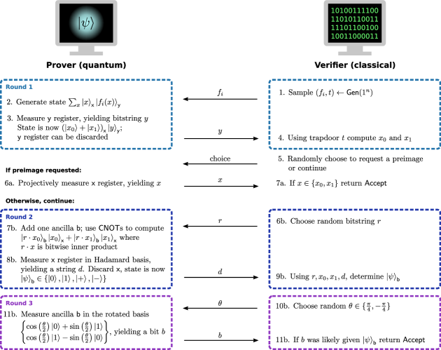
Figure 1: Schematic representation of the interactive quantum advantage protocol. In the first round of interaction, the classical verifier (right) selects a specific function from a trapdoor claw-free family and the quantum prover (left) evaluates it over a superposition of inputs. The goal of the second round is to condense the information contained in the prover’s superposition state onto a single ancilla qubit. The final round of interaction effectively performs a Bell inequality measurement, whose outcome is cryptographically protected.

Recently, a beautiful interactive protocol was introduced that can operate both as a test for quantum advantage and as a generator of certifiable quantum randomness [17]. The core of the protocol is a two-to-one function, $f$, built on the computational problem known as learning with errors (LWE) [25]. The demonstration of advantage leverages two important properties of the function: first, it is claw-free, meaning that it is computationally hard to find a pair of inputs $(x_{0},x_{1})$ such that $f(x_{0})=f(x_{1})$. . Second, there exists a trapdoor: given some secret data $t$, it becomes possible to efficiently invert $f$ and reveal the pair of inputs mapping to any output. (See supplemental information [27] for an overview of trapdoor claw-free functions). However, to fully protect against cheating provers, the protocol requires a stronger version of the claw-free property called the adaptive hardcore bit, namely, that for any input $x_{0}$ (which may be chosen by the prover), it is computationally hard to find even a single bit of information about $x_{1}$ . The need for an adaptive hardcore bit within this protocol severely restricts the class of functions that can operate as verifiable tests of quantum advantage.

Here, we propose and analyze a novel interactive quantum advantage protocol that removes the need for an adaptive hardcore bit, with essentially zero overhead in the quantum circuit and no extra cryptographic assumptions. We present four main results. First, we demonstrate how an idea from tests of Bell’s inequality can serve the same cryptographic purpose as the adaptive hardcore bit [29]. In essence, our interactive protocol is a variant of the CHSH (Clauser, Horne, Shimony, Holt) game [30] in which one player is replaced by a cryptographic construction. Normally, in CHSH, two quantum parties are asked to produce correlations that would be impossible for classical devices to produce. If space-like separation is enforced to rule out communication between the two parties, then the correlations constitute a proof of quantumness. In our case, the space-like separation is replaced by the computational hardness of a cryptographic problem. In particular, the quantum prover holds a qubit whose state depends on the cryptographic secret in the same way that the state of one CHSH player’s qubit depends on the secret measurement basis of the other player. An alternative interpretation, from the perspective of Bell’s theorem, is that the protocol can be thought of as a “single-detector Bell test”—the cryptographic task generates the same single-qubit state as would be produced by entangling a second qubit and measuring it with another detector. As in the CHSH game, a quantum device can pass the verifier’s test with probability $\sim 85\%$, but a classical device can only succeed with probability at most $75\%$. This finite gap in success probabilities is precisely what enables a verifiable test of quantum advantage.

Second, by removing the need for an adaptive hardcore bit, our protocol accepts a broader landscape of functions for interactive tests of quantum advantage (see Table 1 and Methods). We populate this list with two new constructions. The first is based on the decisional Diffie-Hellman problem (DDH) [31, 32, 33]; the second utilizes the function $f_{N}(x)=x^{2}\bmod N$ with $N$ the product of two primes, which forms the backbone of the Rabin cryptosystem [34, 35]. On the one hand, DDH is appealing because the elliptic-curve version of the problem is particularly hard for classical computers [36, 37, 38]. On the other hand, $x^{2}\bmod N$ can be implemented significantly more efficiently, while its hardness is equivalent to factoring. We hope that these two constructions will provide a foundation for the search for more TCFs with desirable properties (small key size and efficient quantum circuits).

Third, we describe two innovations that facilitate our protocol’s use in practice: a way to significantly reduce overhead arising from the reversibility requirement of quantum circuits, and a scheme for increasing noisy devices’ probability of passing the test. Normally, quantum implementations of classical functions like the TCFs used in this protocol have some overhead, due to the need to make the circuit reversible in order to be consistent with unitarity [39, 40, 41, 42, 43]. Our protocol exhibits the surprising property that it permits a measurement scheme to discard so-called “garbage bits” that arise during the computation, allowing classical circuits to be converted into quantum ones with essentially zero overhead. In the case of a noisy quantum device, the protocol also enables an inherent post-selection scheme for detecting and removing certain types of quantum errors. With this scheme it is possible for quantum devices to trade off low quantum fidelities for an increase in the overall runtime, while still passing the cryptographic test. We note that these constructions are likely applicable to other TCF-based quantum cryptography protocols as well, and thus may be of independent interest for tasks such as certifiable quantum random number generation.

Finally, focusing on the TCF $x^{2}\bmod N$, we provide explicit quantum circuits—both asymptotically optimal (requiring only $\mathcal{O}(n\log n)$ gates and $\mathcal{O}(n)$ qubits), as well as those aimed for near-term quantum devices. We show that a verifiable test of quantum advantage can be achieved with $\sim 10^{3}$ qubits and a gate depth $\sim 10^{5}$ (see Methods). We also co-design a specific implementation of $x^{2}\bmod N$ optimized for a programmable Rydberg-based quantum computing platform. The native physical interaction corresponding to the Rydberg blockade mechanism enables the direct implementation of multi-qubit-controlled arbitrary phase rotations without the need to decompose such gates into universal two-qubit operations [44, 45, 46, 47, 48]. Access to such a native gate immediately reduces the gate depth for achieving quantum advantage by an order of magnitude.

Problem	Trap door	Claw- free	Adaptive hard-core bit	Asymptotic complexity (gate count)
LWE [17]	✓	✓	✓	$n^{2}\log^{2}n$
$x^{2}\bmod N$	✓	✓	✗	$n\log n$
Ring-LWE [18]	✓	✓	✗	$n\log^{2}n$
Diffie-Hellman	✓	✓	✗	$n^{3}\log^{2}n$
Shor’s alg.	—	—	—	$n^{2}\log n$

Table 1: Cryptographic constructions for interactive quantum advantage protocols. $n$ represents the number of bits in the function’s input string. Big-$\mathcal{O}$ notation is implied and factors of $\log\log n$ and smaller are dropped. For references and derivations of the circuit complexities, see supplementary information [27].

II Background and Related work

The use of trapdoor claw-free functions for quantum cryptographic tasks was pioneered in two recent breakthrough protocols: (i) giving classical homomorphic encryption for quantum circuits [49] and (ii) for generating cryptographically certifiable quantum randomness from an untrusted black-box device [17]; this latter work also introduced the notion of an adaptive hardcore bit and serves as an efficiently verifiable test of quantum advantage. Remarkably, the scheme was further extended to allow a classical server to cryptographically verify the correctness of arbitrary quantum computations [50]; it has also been applied to remote state preparation with implications for secure delegated computation [51].

Recently, an improvement to the practicality of TCF-based proofs of quantumness was provided in the random oracle model (ROM)—a model of computation in which both the quantum prover and classical verifier can query a third-party “oracle,” which returns a random (but consistent) output for each input. In that work, the authors provide a protocol that both removes the need for the adaptive hardcore bit, and also reduces the interaction to a single round [18]. Because the security of the protocol is proven in the ROM, implementing this protocol in practice requires applying the random oracle heuristic, in which the random oracle is replaced by a cryptographic hash function, but the hardness of classically defeating the protocol is taken to still hold . Only contrived cryptographic schemes have ever been broken by attacking the random oracle heuristic [53, 54], so it seems to be effective in practice and the ROM protocol has significant potential for use as a practical tool for benchmarking untrusted quantum servers. On the other hand, for a robust experimental test of the foundational complexity theoretic claims of quantum computing—that quantum mechanics allows for algorithms that are superpolynomially faster than classical Turing machines—we desire the complexity-theoretic backing of the speedup to be as strong as possible (i.e. provable in the “standard model” of computation [55]), which is the goal pursued in the present work. With that said, we emphasize that the various optimizations described below—including the TCF families based on DDH and $x^{2}\bmod N$, as well as the schemes for postselection and discarding garbage bits—can be applied to the ROM protocol as well.

Lastly, we also note two recent works which demonstrate that any TCF-based proof of quantumness, including the present work, can be implemented in constant quantum circuit depth (at the cost of more qubits) [56, 57].

III Interactive Protocol for Quantum Advantage

Our full protocol is shown diagrammatically in Figure 1. It consists of three rounds of interaction between the prover and verifier (with a “round” being a challenge from the verifier, followed by a response from the prover). The first round generates a multi-qubit superposition over two bit strings that would be cryptographically hard to compute classically. The second round maps this superposition onto the state of one ancilla qubit, retaining enough information to ensure that the resulting single-qubit state is also hard to compute classically. The third round takes this single qubit as input to a CHSH-type measurement, allowing the prover to generate a bit of data that is correlated with the cryptographic secret in a way that would not be possible classically. Having described the intuition behind the protocol, we now lay out each round in detail.

III.1 Description of the protocol

The goal of the first round is to generate a superposition over two colliding inputs to the trapdoor claw-free function (TCF). It begins with the verifier choosing an instance $f_{i}$ of the TCF along with the associated trapdoor data $t$; $f_{i}$ is sent to the prover. As an example, in the case of $x^{2}\mod N$, the “index” $i$ is the modulus $N$, and the trapdoor data is its factorization, $p,q$. The prover now initializes two registers of qubits, which we denote as the $\mathsf{x}$ and $\mathsf{y}$ registers. On these registers, they compute the entangled superposition $\ket{\psi}=\sum_{x}\ket{x}_{\mathsf{x}}\ket{f_{i}(x)}_{\mathsf{y}}$, over all $x$ in the domain of $f_{i}$. The prover then measures the $\mathsf{y}$ register in the standard basis, collapsing the state to $\left(\ket{x_{0}}+\ket{x_{1}}\right)_{\mathsf{x}}\ket{y}_{\mathsf{y}}$, with $y=f(x_{0})=f(x_{1})$. The measured bitstring $y$ is then sent to the verifier, who uses the secret trapdoor to compute $x_{0}$ and $x_{1}$ in full.

At this point, the verifier randomly chooses to either request a projective measurement of the $\mathsf{x}$ register, ending the protocol, or to continue with the second and third rounds. In the former case, the prover communicates the result of that measurement, yielding either $x_{0}$ or $x_{1}$, and the verifier checks that indeed $f(x)=y$. In the latter case, the protocol proceeds with the final two rounds.

The second round of interaction converts the many-qubit superposition $\ket{\psi}=\ket{x_{0}}_{\mathsf{x}}+\ket{x_{1}}_{\mathsf{x}}$ into a single-qubit state $\{\ket{0}_{\mathsf{b}},\ket{1}_{\mathsf{b}},\ket{+}_{\mathsf{b}},\ket{-}_{\mathsf{b}}\}$ on an ancilla qubit $\mathsf{b}$. The final state of $\mathsf{b}$ depends on the values of both $x_{0}$ and $x_{1}$. The round begins with the verifier choosing a random bitstring $r$ of the same length as $x_{0}$ and $x_{1}$, and sending it to the prover. Using a series of CNOT gates from the $\mathsf{x}$ register to $\mathsf{b}$, the prover computes the state $\ket{r\cdot x_{0}}_{\mathsf{b}}\ket{x_{0}}_{\mathsf{x}}+\ket{r\cdot x_{1}}_{\mathsf{b}}\ket{x_{1}}_{\mathsf{x}}$, where $r\cdot x$ denotes the binary inner product. Finally, the prover measures the $\mathsf{x}$ register in the Hadamard basis, storing the result as a bitstring $d$ which is sent to the verifier. This measurement disentangles $\mathsf{x}$ from $\mathsf{b}$ without collapsing $\mathsf{b}$’s superposition. At the end of the second round, the prover’s state is $(-1)^{d\cdot x_{0}}\ket{r\cdot x_{0}}_{\mathsf{b}}+(-1)^{d\cdot x_{1}}\ket{r\cdot x_{1}}_{\mathsf{b}}$, which is one of $\{\ket{0},\ket{1},\ket{+},\ket{-}\}$. Crucially, it is cryptographically hard to predict whether this state is one of $\{\ket{0},\ket{1}\}$ or $\{\ket{+},\ket{-}\}$.

The final round of our protocol can be understood in analogy to the CHSH game [30]. While the prover cannot extract the polarization axis from their single qubit (echoing the no-signaling property of CHSH), they can make a measurement that is correlated with it. This measurement outcome ultimately constitutes the proof of quantumness. In particular, the verifier requests a measurement in an intermediate basis, rotated from the $Z$ axis around $Y$, by either $\theta=\pi/4$ or $-\pi/4$. Because the measurement basis is never perpendicular to the state, there will always be one outcome that is more likely than the other (specifically, with probability $\cos^{2}(\pi/8)\approx 0.85$). The verifier returns $\mathsf{Accept}$ if this “more likely” outcome is the one received.

In the next section, we prove that a quantum device can cause the verifier to $\mathsf{Accept}$ with substantially higher probability than any classical prover. A full test of quantum advantage would consist of running the protocol many times, until it can be established with high statistical confidence that the device has exceeded the classical probability bound.

III.2 Completeness and soundness

We now prove completeness (the noise-free quantum success probability) and soundness (an upper bound on the classical success probability). Recall that after the first round of the protocol, the verifier chooses to either request a standard basis measurement of the first register, or to continue with the second and third rounds. In the proofs below, we analyze the prover’s success probability across these two cases separately. We denote the probability that the verifier will accept the prover’s string $x$ in the first case as $p_{x}$, and the probability that the verifier will accept the single-qubit measurement result in the second case as $p_{\mathrm{CHSH}}$.

III.2.1 Perfect quantum prover (completeness)

Theorem 1.

An error-free quantum device honestly following the interactive protocol will cause the verifier to return $\mathsf{Accept}$ with $p_{x}=1$ and $p_{\mathrm{CHSH}}=\cos^{2}\left(\pi/8\right)\approx 0.85$.

Proof.

If the verifier chooses to request a projective measurement of $\mathsf{x}$ after the first round, an honest quantum prover succeeds with probability $p_{x}=1$ by inspection.

If the verifier chooses to instead perform the rest of the protocol, the prover will hold one of $\{\ket{0},\ket{1},\ket{+},\ket{-}\}$ after round 2. In either measurement basis the verifier may request in round 3, there will be one outcome that occurs with probability $\cos^{2}\left(\pi/8\right)$, which is by construction the one the verifier accepts. Thus, an honest quantum prover has $p_{\mathrm{CHSH}}=\cos^{2}(\pi/8)\approx 0.85$. ∎

III.2.2 Classical prover (soundness)

thmclassicalhardness Assume the function family used in the interactive protocol is claw-free. Then, $p_{x}$ and $p_{\mathrm{CHSH}}$ for any classical prover must obey the relation

$$p_{x}+4p_{\mathrm{CHSH}}-4<\epsilon(n)$$ (1)

where $\epsilon$ is a negligible function of $n$, the length of the function family’s input strings.

Proof.

We prove by contradiction. Assume that there exists a classical machine $\mathcal{A}$ for which $p_{x}+4p_{\mathrm{CHSH}}-4\geq\mu(n)$, for a non-negligible function $\mu$. We show that there exists another algorithm $\mathcal{B}$ that uses $\mathcal{A}$ as a subroutine to find a pair of colliding inputs to the claw-free function, a contradiction.

Given a claw-free function instance $f_{i}$, $\mathcal{B}$ acts as a simulated verifier for $\mathcal{A}$. $\mathcal{B}$ begins by supplying $f_{i}$ to $\mathcal{A}$, after which $\mathcal{A}$ returns a value $y$, completing the first round of interaction. $\mathcal{B}$ now chooses to request the projective measurement of the $x$ register, and stores the result as $x_{0}$. Letting $p_{x_{0}}$ be the probability that $x_{0}$ is a valid preimage, by definition of $p_{x}$ we have $p_{x_{0}}=p_{x}$.

Next, $\mathcal{B}$ rewinds the execution of $\mathcal{A}$, to its state before $x_{0}$ was requested. Crucially, rewinding is possible because $\mathcal{A}$ is a classical algorithm. $\mathcal{B}$ now proceeds by running $\mathcal{A}$ through the second and third rounds of the protocol for many different values of the bitstring $r$ (Fig. 1), rewinding each time.

We now show that, for $r$ selected uniformly at random, $\mathcal{B}$ can extract the value of the inner product $r\cdot x_{1}$ with probability $p_{r\cdot x_{1}}\geq 1-2(1-p_{\mathrm{CHSH}})$. $\mathcal{B}$ begins by sending $r$ to $\mathcal{A}$, and receiving the bitstring $d$. $\mathcal{B}$ then requests the measurement result in both the $\theta=\pi/4$ and $\theta=-\pi/4$ bases, by rewinding in between. Supposing that both the received values are “correct” (i.e. would be accepted by the real verifier), they uniquely determine the single-qubit state $\ket{\psi}\in\{\ket{0},\ket{1},\ket{+},\ket{-}\}$ that would be held by an honest quantum prover. This state reveals whether $r\cdot x_{0}=r\cdot x_{1}$, and because $\mathcal{B}$ already holds $x_{0}$, $\mathcal{B}$ can compute $r\cdot x_{1}$. We may define the probability (taken over all randomness except the choice of $\theta$) that the prover returns an accepting value in the cases $\theta=\pi/4$ and $\theta=-\pi/4$ as $p_{\pi/4}$ and $p_{-\pi/4}$ respectively. Then, via union bound, the probability that both are indeed correct is $p_{r\cdot x_{1}}\geq 1-(1-p_{\pi/4})-(1-p_{-\pi/4})$. Considering that $p_{\mathrm{CHSH}}=(p_{\pi/4}+p_{-\pi/4})/2$, we have $p_{r\cdot x_{1}}\geq 1-2(1-p_{\mathrm{CHSH}})$.

Now, we show that extracting $r\cdot x_{1}$ in this way allows $x_{1}$ to be determined in full even in the presence of noise, by rewinding many times and querying for specific (correlated) choices of $r$. In particular, the above construction is a noisy oracle to the encoding of $x_{1}$ under the Hadamard code. By the Goldreich-Levin theorem [58], list decoding applied to such an oracle will generate a polynomial-length list of candidates for $x_{1}$. If the noise rate of the oracle is noticeably less than $1/2$, $x_{1}$ will be contained in that list; $\mathcal{B}$ can iterate through the candidates until it finds one for which $f(x_{1})=y$.

By Lemma 1 in the Methods, for a particular iteration of the protocol, the probability that list decoding succeeds is bounded by $p_{x_{1}}>2p_{r\cdot x_{1}}-1-2\mu^{\prime}(n)$, for a noticeable function $\mu^{\prime}(n)$ of our choice . Setting $\mu^{\prime}(n)=\mu(n)/4$ and combining with the previous result yields $p_{x_{1}}>1-4(1-p_{\mathrm{CHSH}})-\mu(n)/2$.

Finally, via union bound, the probability that $\mathcal{B}$ returns a claw is

$${P}_{\mathcal{B}}\geq 1-(1-p_{x_{0}})-(1-p_{x_{1}})>p_{x}+4p_{\mathrm{CHSH}}-4-\mu(n)/2$$

and via the assumption that $p_{x}+4p_{\mathrm{CHSH}}-4>\mu(n)$ we have

$${P}_{\mathcal{B}}>\mu(n)/2$$

a contradiction. ∎

If we let $p_{x}=1$, the bound requires that $p_{\mathrm{CHSH}}<3/4+\epsilon(n)$ for a classical device, while $p_{\mathrm{CHSH}}\approx 0.85$ for a quantum device, matching the classical and quantum success probabilities of the CHSH game. In the supplementary information [27], we provide an example of a classical algorithm saturating the bound with $p_{x}=1$ and $p_{\mathrm{CHSH}}=3/4$.

III.3 Robustness: Error mitigation via postselection

The existence of a finite gap between the classical and quantum success probabilities implies that our protocol can tolerate a certain amount of noise. A direct implementation of our interactive protocol on a noisy quantum device would require an overall fidelity of $\sim 83$% in order to exceed the classical bound . To allow devices with lower fidelities to demonstrate quantum advantage, our protocol allows for a natural tradeoff between fidelity and runtime, such that the classical bound can, in principle, be exceeded with only a small [e.g. $1/\mathrm{poly}(n)$] amount of coherence in the quantum device .

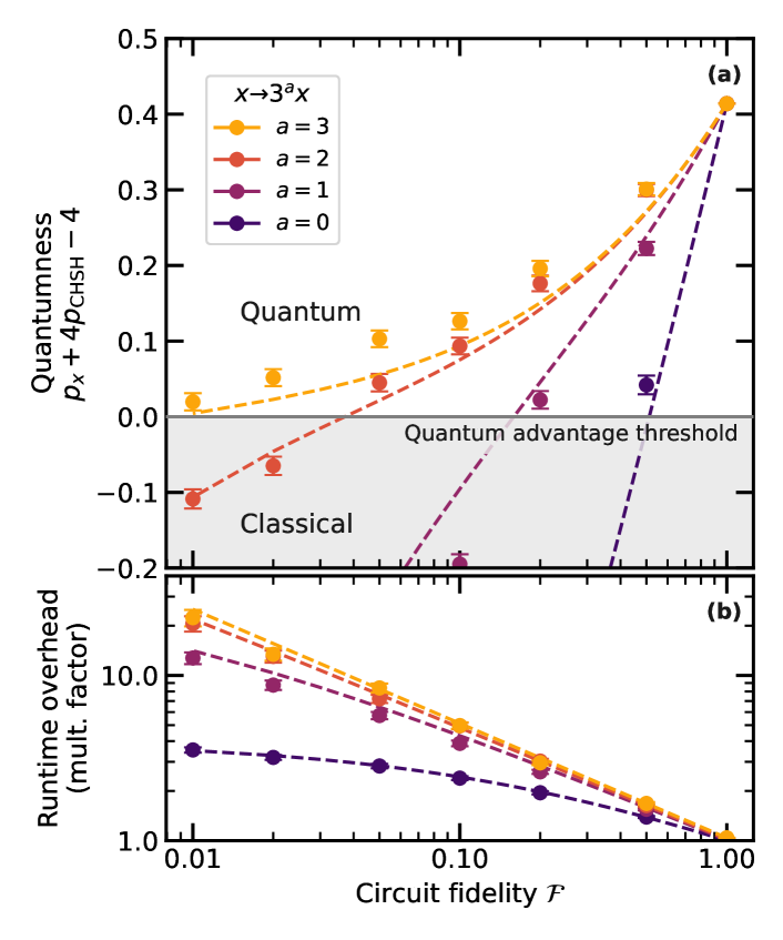
Figure 2: Performance of our post-selection scheme when redundancy is added to the function $x^{2}\bmod N$ by mapping it to $(3^{a}x)^{2}\bmod 3^{2a}N$. Numerical simulations are performed on a quantum circuit implementing the Karatsuba algorithm for $a=\{{0,1,2,3}\}$ (see supplemental information [27]). (a) “Quantumness” measured in terms of the classical bound from Eqn. 1 as a function of the total circuit fidelity. With $a=3$, even a quantum device with only 1% circuit fidelity can demonstrate quantum advantage. (b) Depicts the increased runtime associated the post-selection scheme, which arises from a combination of slightly larger circuit sizes and the need to re-run the circuit multiple times. The latter is by far the dominant effect. Dashed lines are a theory prediction with no fit parameters; points are the result of numerical simulations at $n=512$ bits and error bars depict $2\sigma$ uncertainty.

The key idea is based upon postselection. For most TCFs, there are many bitstrings of the correct length that are not valid outputs of $f$. Thus, if the prover detects such a $y$ value in step 3 (Fig. 1), they can simply discard it and try again . In principle, the verifier can even use their trapdoor data to silently detect and discard iterations of the protocol with invalid $y$ . Since $y$ is a function of $x_{0}$ and $x_{1}$, one might hope that this postselection scheme also rejects states where $x_{0}$ or $x_{1}$ has become corrupt. Although this may not always be the case, we demonstrate numerically that this assumption holds for a specific implementation of $x^{2}\bmod N$ in the following subsection. One could also compute a classical checksum of $x_{0}$ and $x_{1}$ before and after the main circuit to ensure that they have not changed during its execution. Assuming that such bit-flip errors are indeed rejected, the possibility remains of an error in the phase between $\ket{x_{0}}$ and $\ket{x_{1}}$. In the supplementary information [27], we demonstrate that a prover holding the correct bitstrings but with an error in the phase can still saturate the classical bound; if the prover can avoid phase errors even a small fraction of the time, they will push past the classical threshold.

III.3.1 Numerical analysis of the postselection scheme for $x^{2}\bmod N$

Focusing on the function $f(x)=x^{2}\bmod N$, we now explicitly analyze the effectiveness of the postselection scheme. Let $m$ be the length of the outputs of this function. In this case, approximately $1/4$ of the bitstrings of length $m$ are valid outputs, so one would naively expect to reject about $3/4$ of corrupted bitstrings. By introducing additional redundancy into the outputs of $f$ and thus increasing $m$, one can further decrease the probability that a corrupted $y$ will incorrectly be accepted. As an example, let us consider mapping $x^{2}\bmod N$ to the function $(kx)^{2}\bmod k^{2}N$ for some integer $k$. This is particularly convenient because the prover can validate $y$ by simply checking whether it is a multiple of $k^{2}$. Moreover, the mapping adds only $\log k$ bits to the size of the problem, while rejecting a fraction $1-1/k^{2}$ of corrupted bitstrings.

We perform extensive numerical simulations demonstrating that postselection allows for quantum advantage to be achieved using noisy devices with low circuit fidelities (Fig. 2). We simulate quantum circuits for $(kx)^{2}\bmod k^{2}N$ at a problem size of $n=512$ bits. Assuming a uniform gate fidelity across the circuit, we analyze the success rate of a quantum prover for $k=3^{a}$ and $a=\{0,1,2,3\}$. For these simulations we use our implementation of the Karatsuba algorithm (see Section IV.1) because it is the most efficient in terms of gate count and depth. The choice of $k=3^{a}$, and details of the simulation, are explained in the supplementary information [27].

For $a=0$, the circuit implements our original function $x^{2}\bmod N$, where in the absence of postselection, an overall circuit fidelity of $\mathcal{F}\sim 0.83$ is required to achieve quantum advantage. As depicted in Fig. 2(a), even for $a=0$, our postselection scheme improves the advantage threshold down to $\mathcal{F}\sim 0.51$. For $a=2$, circuit fidelities with $\mathcal{F}\gtrsim 0.1$ remain well above the quantum advantage threshold, while for $a=3$ the required circuit fidelity drops below $1\%$.

However, there is a tradeoff. In particular, one expects the overall runtime to increase for two reasons: (i) there will be a slight increase in the circuit size for $a>0$ and (ii) one may need to re-run the quantum circuit many times until a valid $y$ is measured. Somewhat remarkably, a runtime overhead of only $4.7$x already enables quantum advantage to be achieved with an overall circuit fidelity of $10\%$ [Fig. 2(b)]. Crucially, this increase in runtime is overwhelmingly due to re-running the quantum circuit and does not imply the need for longer experimental coherence times.

III.4 Efficient quantum evaluation of irreversible classical circuits

The central computational step in our interactive protocol (i.e. step 2, Fig. 1) is for the prover to apply a unitary of the form:

$$\mathcal{U}_{f_{i}}\sum_{x}\ket{x}_{\mathsf{x}}\ket{0^{\otimes m}}_{\mathsf{y}}=\sum_{x}\ket{x}_{\mathsf{x}}\ket{f_{i}(x)}_{\mathsf{y}},$$ (2)

where $f_{i}(x)$ is a classical function and $m$ is the length of the output register. This type of unitary operation is ubiquitous across quantum algorithms, and a common strategy for its implementation is to convert the gates of a classical circuit into quantum gates. Generically, this process induces substantial overhead in both time and space complexity owing to the need to make the circuit reversible to preserve unitarity [39, 40]. This reversibility is often achieved by using an additional register, $\mathsf{g}$, of so-called “garbage bits” and implementing: $\mathcal{U}_{f_{i}}^{\prime}\sum_{x}\ket{x}_{\mathsf{x}}\ket{0^{\otimes m}}_{\mathsf{y}}\ket{0^{\otimes l}}_{\mathsf{g}}=\sum_{x}\ket{x}_{\mathsf{x}}\ket{f_{i}(x)}_{\mathsf{y}}\ket{g_{i}(x)}_{\mathsf{g}}$. For each gate in the classical circuit, enough garbage bits are added to make the operation injective. In general, to maintain coherence, these bits cannot be discarded but must be “uncomputed” later, adding significant complexity to the circuits.

A particularly appealing feature of our protocol is the existence of a measurement scheme to discard garbage bits, allowing for the direct mapping of classical to quantum circuits with no overhead. Specifically, we envision the prover measuring the qubits of the $\mathsf{g}$ register in the Hadamard basis and storing the results as a bitstring $h$, yielding the state,

$$\ket{\psi}=\sum_{x}(-1)^{h\cdot g_{i}(x)}\ket{x}_{\mathsf{x}}\ket{f_{i}(x)}_{\mathsf{y}}.$$ (3)

The prover has avoided the need to do any uncomputation of the garbage bits, at the expense of introducing phase flips onto some elements of the superposition. These phase flips do not affect the protocol, so long as the verifier can determine them. While classically computing $h\cdot g_{i}(x)$ is efficient for any $x$, computing it for all terms in the superposition is infeasible for the verifier. However, our protocol provides a natural way around this. The verifier can wait until the prover has collapsed the superposition onto $x_{0}$ and $x_{1}$, before evaluating $g_{i}(x)$ only on those two inputs .

Crucially, the prover can measure away garbage qubits as soon as they would be discarded classically, instead of waiting until the computation has completed. If these qubits are then reused, the quantum circuit will use no more space than the classical one. This feature allows for significant improvements in both gate depth and qubit number for practical implementations of the protocol (see last rows of Table I in Methods). We note that performing many individual measurements on a subset of the qubits is difficult on some experimental systems, which may make this technique challenging to use in practice. However, recent hardware advances have demonstrated these “intermediate measurements” in practice with high fidelity, for example by spatially shuttling trapped ions [65, 66]. We thus expect that the capability to perform partial measurements will not be a barrier in the near term. This issue can also be mitigated somewhat by collecting ancilla qubits and measuring them in batches rather than one-by-one, allowing for a direct trade-off between ancilla usage and the number of partial measurements.

IV Quantum circuits for trapdoor claw-free functions

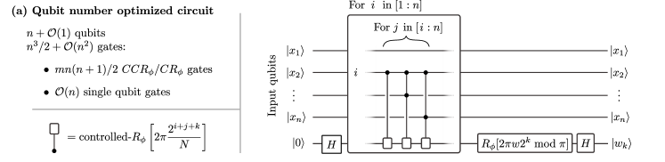
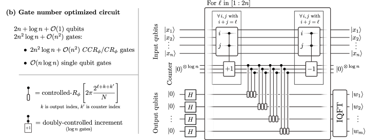
Figure 3: Quantum circuits implementing step 2 of our interactive protocol for $f(x)=x^{2}\bmod N$. $n$ is the length of the input register, and $m=n+\mathcal{O}(1)$ is the length of the output register. (a) Depicts a quantum circuit optimized for qubit number. The circuit shown computes the $k^{\mathrm{th}}$ bit of $w=x^{2}/N$ and should be iterated for $k$. This iteration should begin at the least significant bit to ensure that the final phase rotation can be estimated classically. Note that the only entangling operations necessary for the circuit are doubly-controlled gates, which can be natively implemented using the Rydberg blockade (see Section IV.2). (b) Depicts a quantum circuit optimized for gate number. By combining gates of equal phase, one can reduce the overall circuit complexity to $\mathcal{O}(n^{2}\log n)$ gates. We note that neither circuit requires use of the “garbage bit” procedure described in Section III.4; this design choice reduces measurement complexity. If desired, that procedure could be applied to the counter register of circuit (b) in place of the controlled-decrement operation.

While all of the trapdoor, claw-free functions listed in Table 1 can be utilized within our interactive protocol, each has its own set of advantages and disadvantages. For example, the TCF based on the Diffie-Hellman problem (described in the Methods) already enables a demonstration of quantum advantage at a key size of 160 bits (with a hardness equivalent to 1024 bit integer factorization [38]); however, building a circuit for this TCF requires a quantum implementation of Euclid’s algorithm, which is challenging [67]. Thus, we focus on designing quantum circuits implementing Rabin’s function, $x^{2}\bmod N$.

IV.1 Quantum circuits for $x^{2}\bmod N$

We explore four different circuits (implementations of these algorithms in Python using the Cirq library are included as supplementary files ). The first two are quantum implementations of the Karatsuba and “schoolbook” classical integer multiplication algorithms, where we leverage the reversibility optimizations described in Section III.4 (see supplementary information [27]). The latter pair, which we call the “phase circuits” and describe below, are intrinsically quantum algorithms that use Ising interactions to directly compute $x^{2}\bmod N$ in the phase. Using those circuits, we propose a near-term demonstration of our interactive protocol on a Rydberg-based quantum computer [45, 48]; crucially, the so-called “Rydberg blockade” interaction natively realizes multi-qubit controlled phase rotations, from which the entire circuits shown in Figure 3 are built (up to single qubit rotations). A comparison of approximate gate counts for each of the four circuits can be seen in Table I in the Methods. The Karatsuba algorithm is the most efficient in total gates and circuit depth, while the phase circuits are most efficient in terms of qubit usage and measurement complexity.

We now describe the two circuits, amenable to near-term quantum devices, that utilize quantum phase estimation to implement the function $f(x)=x^{2}\bmod N$. The intuition behind our approach is as follows: we will compute $x^{2}/N$ in the phase and transfer it to an output register via an inverse quantum Fourier transform [69, 70]; the modulo operation occurs automatically as the phase wraps around the unit circle, avoiding the need for a separate reduction step.

In order to implement $\sum_{x}\ket{x}_{\mathsf{x}}\ket{x^{2}\bmod N}_{\mathsf{y}}$, we design a circuit to compute:

$$(\mathbb{I}\otimes\mathrm{IQFT})\;\tilde{\mathcal{U}}_{w_{N}}\;(\mathbb{I}\otimes\mathrm{H^{\otimes m}})\ket{x}\ket{0^{\otimes m}}=\ket{x}\ket{w}$$ (4)

where $\mathrm{H}$ is a Hadamard gate, $\mathrm{IQFT}$ represents an inverse quantum Fourier transform, $w\equiv x^{2}/N=0.w_{1}w_{2}\cdots w_{m}$ is an $m$-bit binary fraction , and $\tilde{\mathcal{U}}_{w_{N}}$ is the diagonal unitary,

$$\tilde{\mathcal{U}}_{w_{N}}\ket{x}\ket{z}=\exp\left(2\pi i\frac{x^{2}}{N}z\right)\ket{x}\ket{z}.$$ (5)

By performing a binary decomposition of the phase in Eqn. 5:

$$\exp{\left(2\pi i\frac{x^{2}}{N}z\right)}=\prod_{i,j,k}\exp{\left(2\pi i\frac{2^{i+j+k}}{N}x_{i}x_{j}z_{k}\right)},$$ (6)

one immediately finds that $\tilde{\mathcal{U}}_{w_{N}}$ is equivalent to applying a series of controlled-controlled-phase rotation gates of angle,

$$\phi_{ijk}=\frac{2\pi 2^{i+j+k}}{N}\pmod{2\pi}.$$ (7)

Here, the control qubits are $i,j$ in the $\mathsf{x}$ register, while the target qubit is $k$ in the $\mathsf{y}$ register. Crucially, the value of this phase for any $i,j,k$ can be computed classically when the circuit is compiled.

As depicted in Figure 3, we propose two explicit circuits to implement $\tilde{\mathcal{U}}_{w_{N}}$, one optimizing for qubit count, and the other optimizing for gate count. The first circuit [Fig. 3(a)] takes advantage of the fact that the output register is measured immediately after it is computed; this allows one to replace the $m$ output qubits with a single qubit that is measured and reused $m$ times. Moreover, by replacing groups of doubly-controlled gates with a Toffoli and a series of singly-controlled gates, one ultimately arrives at an implementation, which requires $n^{3}/2+\mathcal{O}(n^{2})$ gates, but only $n+\mathcal{O}(1)$ qubits. We note that this does require individual measurement and re-use of qubits, which has been a challenge for experiments; recent experiments however have demonstrated this capability [65, 66].

Our second circuit [Fig. 3(b)], which optimizes for gate count, leverages the fact that $\phi_{ijk}$ (Eqn. 7) only depends on $i+j+k$, allowing one to combine gates with a common sum. In this case, one can define $\ell=i+j$ and then, for each value of $\ell$, simply “count” the number of values of $i,j$ for which both control qubits are 1. By then performing controlled gates off of the qubits of the counter register, one can reduce the total gate complexity by a factor of $n/\log n$, leading to a implementation with $2n^{2}\log n+\mathcal{O}(n^{2})$ gates.

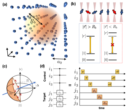
Figure 4: a, Schematic illustration of a three dimensional array of neutral atoms with Rydberg blockade interactions. The blockade radius can be significantly larger than the inter-atom spacing, enabling multi-qubit entangling operations. b, As an example, Rydberg atoms can be trapped in an optical tweezer array. The presence of an atom in a Rydberg excited state (red) shifts the energy levels of nearby atoms (blue), preventing the driving field (yellow arrow) from exciting them to their Rydberg state, $|r\rangle$. c, A single qubit phase rotation can be implemented by an off-resonant Rabi oscillation between one of the qubit states, e.g., $\ket{1}$, and the Rydberg excited state. This imprints a tunable, geometric phase $\phi$, which is determined by the detuning $\Delta$ and Rabi frequency $\Omega$. d, Multi-qubit controlled-phase rotations are implemented via a sequence of $\pi$-pulses between the $\ket{0}\leftrightarrow\ket{r}$ transition of control atoms (yellow) and off-resonant Rabi oscillations on the target atoms (orange).

IV.2 Experimental implementation

Motivated by recent advances in the creation and control of many-body entanglement in programmable quantum systems [72, 11, 73, 74], we propose an experimental implementation of our interactive protocol based upon neutral atoms coupled to Rydberg states [48]. We envision a three dimensional system of either alkali or alkaline-earth atoms trapped in an optical lattice or optical tweezer array [Fig. 4(a)] [75, 76, 77]. To be specific, we consider ${}^{87}\rm Rb$ with an effective qubit degree of freedom encoded in hyperfine states: $\ket{0}=\ket{F=1,m_{F}=0}$ and $\ket{1}=\ket{F=2,m_{F}=0}$. Gates between atoms are mediated by coupling to a highly-excited Rydberg state $\ket{r}$, whose large polarizability leads to strong van der Waals interactions. This microscopic interaction enables the so-called Rydberg “blockade” mechanism—when a single atom is driven to its Rydberg state, all other atoms within a blockade radius, $R_{b}$, become off-resonant from the drive, thereby suppressing their excitation [Fig. 4(a,b)] [44].

Somewhat remarkably, this blockade interaction enables the native implementation of all multi-qubit-controlled phase gates depicted in the circuits in Figure 3. In particular, consider the goal of applying a $C^{k}R^{\ell}_{\phi}$ gate; this gate applies phase rotations, $\{\phi_{1},\phi_{2},\dots,\phi_{\ell}\}$, to target qubits $\{j_{1},j_{2},\dots j_{\ell}\}$ if all $k$ control qubits $\{i_{1},i_{2},\dots i_{k}\}$ are in the $\ket{1}$ state [Fig. 4(d)]. Experimentally, this can be implemented as follows: (i) sequentially apply (in any order) resonant $\pi$-pulses on the $\ket{0}\leftrightarrow\ket{r}$ transition for the $k$ desired control atoms, (ii) off-resonantly drive the $\ket{1}\leftrightarrow\ket{r}$ transition of each target atom with detuning $\Delta$ and Rabi frequency $\Omega$ for a time duration $T=2\pi/(\Omega^{2}+\Delta^{2})^{1/2}$ [Fig. 4(c)], (iii) sequentially apply [in the opposite order as in (i)] resonant $-\pi$-pulses (i.e. $\pi$-pulses with the opposite phase) to the $k$ control atoms to bring them back to their original state. The intuition for why this experimental sequence implements the $C^{k}R^{\ell}_{\phi}$ gate is straightforward. The first step creates a blockade if any of the control qubits are in the $\ket{0}$ state, while the second step imprints a phase, $\phi=\pi(1-\Delta/\sqrt{\Delta^{2}+\Omega^{2}})$, on the $\ket{1}$ state, only in the absence of a blockade. Note that tuning the values of $\phi_{i}$ for each of the target qubits simply corresponds to adjusting the detuning and Rabi frequency of the off-resonant drive in the second step [Fig. 4(c,d)].

Demonstrations of our protocol can already be implemented in current generation Rydberg experiments, where a number of essential features have recently been shown, including: 1) the coherent manipulation of individual qubits trapped in a 3D tweezer array [75, 76], 2) the deterministic loading of atoms in a 3D optical lattice [77], and 3) fast entangling gate operations with fidelities, $F\geq 0.974$ [45, 46, 47]. In order to estimate the number of entangling gates achievable within decoherence time scales, let us imagine choosing a Rydberg state with a principal quantum number $n\approx 70$. This yields a strong van der Waals interaction, $V(\vec{r})=C_{6}/r^{6}$, with a $C_{6}$ coefficient $\sim(2\pi)\,880$ GHz$\cdot\mu$m⁶ [78]. Combined with a coherent driving field of Rabi frequency $\Omega\sim(2\pi)\,1-10$ MHz, the van der Waals interaction can lead to a blockade radius of up to, $R_{b}=\left(C_{6}/\Omega\right)^{1/6}\sim 10\,\mu$m. Within this radius, one can arrange $\sim 10^{2}$ all-to-all interacting qubits, assuming an atom-to-atom spacing of approximately, $a_{0}\approx 2\mu$m . In current experiments, the decoherence associated with the Rydberg transition is typically limited by a combination of inhomogeneous Doppler shifts and laser phase/intensity noise, leading to $1/T_{2}\sim 10-100$ kHz [80, 45, 81]. Taking everything together, one should be able to perform $\sim 10^{3}$ entangling gates before decoherence occurs (this is comparable to the number of two-qubit entangling gates possible in other state-of-the-art platforms [11, 82]). While this falls short of enabling an immediate full-scale demonstration of classically verifiable quantum advantage, we hasten to emphasize that the ability to directly perform multi-qubit entangling operations significantly reduces the cost of implementing our interactive protocol. For example, the standard decomposition of a Toffoli gate uses 6 CNOT gates and 7 $T$ and $T^{\dagger}$ gates, with a gate depth of 12 [83, 84, 85]; an equivalent three qubit gate can be performed in a single step via the Rydberg blockade mechanism.

V Conclusion and Outlook

The interplay between classical and quantum complexities ultimately determines the threshold for any quantum advantage scheme. Here, we have proposed a novel interactive protocol for classically verifiable quantum advantage based upon trapdoor claw-free functions; in addition to proposing two new TCFs [Table 1], we also provide explicit quantum circuits that leverage the microscopic interactions present in a Rydberg-based quantum computer. Our work allows near-term quantum devices to move one step closer toward a loophole-free demonstration of quantum advantage and also opens the door to a number of promising future directions.

First, our proof of soundness only applies to classical adversaries; whether it is possible to extend our protocol’s security to quantum adversaries remains an open question . A quantum-secure proof could enable our protocol’s use in a number of applications, such as certifiable random number generation [17] and the verification of arbitrary quantum computations [50]. Second, our work motivates the search for new trapdoor claw-free functions, which can be evaluated in the smallest possible quantum volume. Cryptographic primitives such as Learning Parity with Noise (LPN), which are designed for use in low-power devices such as RFID cards, represent a promising path forward [87]. More broadly, one could also attempt to build modified protocols, which simplify either the requirements on the cryptographic function or the interactions; interestingly, recent work has demonstrated that using random oracles can remove the need for interactions in a TCF-based proof of quantumness [18]. Finally, while we have focused our experimental discussions on Rydberg atoms, a number of other platforms also exhibit features that facilitate the protocol’s implementation. For example, both trapped ions and cavity-QED systems can allow all-to-all connectivity, while superconducting qubits can be engineered to have biased noise [88]. This latter feature would allow noise to be concentrated into error modes detectable by our proposed post-selection scheme.

We gratefully acknowledge the insights of and discussions with A. Bouland, S. Garg, A. Gheorghiu, Z. Landau, L. Lewis, and T. Vidick. We are particularly indebted to Joonhee Choi for insights about Rydberg-based quantum computing. This work was supported by the NSF QLCI program through grant number OMA-2016245, and the DOD through MURI grant number FA9550-18-1-0161. NYY acknowledges support from the David and Lucile Packard foundation and a Google research award. GDKM acknowledges support from the Department of Defense (DOD) through the National Defense Science & Engineering Graduate Fellowship (NDSEG) Program. SC acknowledges support from the Miller Institute for Basic Research in Science.

References

- Aaronson and Arkhipov [2011] S. Aaronson and A. Arkhipov, in Proceedings of the forty-third annual ACM symposium on Theory of computing, STOC ’11 (Association for Computing Machinery, New York, NY, USA, 2011) pp. 333–342.
- Farhi and Harrow [2016] E. Farhi and A. W. Harrow, arXiv:1602.07674 (2016).
- Bremner et al. [2016] M. J. Bremner, A. Montanaro, and D. J. Shepherd, Physical Review Letters 117, 080501 (2016).
- Lund et al. [2017] A. P. Lund, M. J. Bremner, and T. C. Ralph, npj Quantum Information 3, 1 (2017).
- Harrow and Montanaro [2017] A. W. Harrow and A. Montanaro, Nature 549, 203 (2017).
- Terhal [2018] B. M. Terhal, Nature Physics 14, 530 (2018).
- Boixo et al. [2018] S. Boixo, S. V. Isakov, V. N. Smelyanskiy, R. Babbush, N. Ding, Z. Jiang, M. J. Bremner, J. M. Martinis, and H. Neven, Nature Physics 14, 595 (2018).
- Bouland et al. [2019] A. Bouland, B. Fefferman, C. Nirkhe, and U. Vazirani, Nature Physics 15, 159 (2019).
- Aaronson and Chen [2017] S. Aaronson and L. Chen, in 32nd Computational Complexity Conference (CCC 2017), Leibniz International Proceedings in Informatics (LIPIcs), Vol. 79, edited by R. O’Donnell (Schloss Dagstuhl–Leibniz-Zentrum fuer Informatik, Dagstuhl, Germany, 2017) pp. 22:1–22:67.
- Neill et al. [2018] C. Neill, P. Roushan, K. Kechedzhi, S. Boixo, S. V. Isakov, V. Smelyanskiy, A. Megrant, B. Chiaro, A. Dunsworth, K. Arya, R. Barends, B. Burkett, Y. Chen, Z. Chen, et al., Science 360, 195 (2018).
- Arute et al. [2019] F. Arute, K. Arya, R. Babbush, D. Bacon, J. C. Bardin, R. Barends, R. Biswas, S. Boixo, F. G. S. L. Brandao, D. A. Buell, B. Burkett, Y. Chen, Z. Chen, B. Chiaro, et al., Nature 574, 505 (2019).
- Zhong et al. [2020] H.-S. Zhong, H. Wang, Y.-H. Deng, M.-C. Chen, L.-C. Peng, Y.-H. Luo, J. Qin, D. Wu, X. Ding, Y. Hu, P. Hu, X.-Y. Yang, W.-J. Zhang, H. Li, et al., Science 370, 1460 (2020).
- Bravyi et al. [2018] S. Bravyi, D. Gosset, and R. König, Science 362, 308 (2018).
- Bravyi et al. [2019] S. Bravyi, D. Gosset, R. Koenig, and M. Tomamichel, arXiv:1904.01502 [quant-ph] (2019).
- Note [1] They also have some other caveats: a provable speedup of quantum complexity over classical complexity is promising, but just reading the input may require time, hiding the computational speedup in practice.
- Shor [1997] P. W. Shor, SIAM Journal on Computing 26, 1484 (1997).
- Brakerski et al. [2019] Z. Brakerski, P. Christiano, U. Mahadev, U. Vazirani, and T. Vidick, arXiv:1804.00640 [quant-ph] (2019).
- Brakerski et al. [2020] Z. Brakerski, V. Koppula, U. Vazirani, and T. Vidick, arXiv:2005.04826 [quant-ph] (2020).
- Aharonov et al. [2017] D. Aharonov, M. Ben-Or, E. Eban, and U. Mahadev, arXiv:1704.04487 (2017).
- Watrous [1999] J. Watrous, arXiv:cs/9901015 (1999).
- Kitaev and Watrous [2000] A. Kitaev and J. Watrous, in Proceedings of the thirty-second annual ACM symposium on Theory of computing (2000) pp. 608–617.
- Kobayashi and Matsumoto [2003] H. Kobayashi and K. Matsumoto, Journal of Computer and System Sciences 66, 429 (2003).
- Fitzsimons and Vidick [2015] J. Fitzsimons and T. Vidick, in Proceedings of the 2015 Conference on Innovations in Theoretical Computer Science (2015) pp. 103–112.
- Markov et al. [2018] I. L. Markov, A. Fatima, S. V. Isakov, and S. Boixo, arXiv:1807.10749 (2018).
- Regev [2005] O. Regev, in Proceedings of the thirty-seventh annual ACM symposium on Theory of computing, STOC ’05 (Association for Computing Machinery, New York, NY, USA, 2005) pp. 84–93.
- Note [2] “Claw-free” is often used to refer to a pair of functions such that for appropriate we have . Here, we use the slightly more general idea of a single 2-to-1 function for which it is hard to find such that . This is a special case of a “collision-resistant function,” which could potentially be many-to-one. We also note that a claw-free pair of functions can be converted into a single claw-free function by defining , where denotes concatenation.
- [27] See Supplementary Information for additional details and supporting derivations.
- Note [3] To be precise, it is hard to find both and the parity of any subset of the bits of .
- Bell [1964] J. S. Bell, Physics Physique Fizika 1, 195 (1964).
- Clauser et al. [1969] J. F. Clauser, M. A. Horne, A. Shimony, and R. A. Holt, Physical Review Letters 23, 880 (1969).
- Diffie and Hellman [1976] W. Diffie and M. Hellman, IEEE Transactions on Information Theory 22, 644 (1976).
- Peikert and Waters [2008] C. Peikert and B. Waters, in Proceedings of the fortieth annual ACM symposium on Theory of computing, STOC ’08 (Association for Computing Machinery, New York, NY, USA, 2008) pp. 187–196.
- Freeman et al. [2010] D. M. Freeman, O. Goldreich, E. Kiltz, A. Rosen, and G. Segev, in Public Key Cryptography – PKC 2010, Lecture Notes in Computer Science, edited by P. Q. Nguyen and D. Pointcheval (Springer, Berlin, Heidelberg, 2010) pp. 279–295.
- Rabin [1979] M. O. Rabin, Digitalized signatures and public-key functions as intractable as factorization, Technical Report (Massachusetts Institute of Technology, USA, 1979).
- Goldwasser et al. [1988] S. Goldwasser, S. Micali, and R. L. Rivest, SIAM Journal on Computing 17, 281 (1988).
- Miller [1986] V. S. Miller, in Advances in Cryptology — CRYPTO ’85 Proceedings, Lecture Notes in Computer Science, edited by H. C. Williams (Springer, Berlin, Heidelberg, 1986) pp. 417–426.
- Koblitz [1987] N. Koblitz, Mathematics of Computation 48, 203 (1987).
- Barker [2016] E. Barker, Recommendation for Key Management Part 1: General, Tech. Rep. NIST SP 800-57pt1r4 (National Institute of Standards and Technology, 2016).
- Bennett [1989] C. H. Bennett, SIAM Journal on Computing 18, 766 (1989).
- Levine and Sherman [1990] R. Y. Levine and A. T. Sherman, SIAM Journal on Computing 19, 673 (1990).
- Aharonov et al. [1998] D. Aharonov, A. Kitaev, and N. Nisan, in Proceedings of the thirtieth annual ACM symposium on Theory of computing (1998) pp. 20–30.
- Babu et al. [2004] H. M. H. Babu, M. R. Islam, S. M. A. Chowdhury, and A. R. Chowdhury, in 17th International Conference on VLSI Design. Proceedings. (IEEE, 2004) pp. 757–760.
- Kotiyal et al. [2014] S. Kotiyal, H. Thapliyal, and N. Ranganathan, in 2014 27th international conference on VLSI design and 2014 13th international conference on embedded systems (IEEE, 2014) pp. 545–550.
- Saffman [2016] M. Saffman, Journal of Physics B: Atomic, Molecular and Optical Physics 49, 202001 (2016).
- Levine et al. [2019] H. Levine, A. Keesling, G. Semeghini, A. Omran, T. T. Wang, S. Ebadi, H. Bernien, M. Greiner, V. Vuletić, H. Pichler, and M. D. Lukin, Phys. Rev. Lett. 123, 170503 (2019).
- Graham et al. [2019] T. Graham, M. Kwon, B. Grinkemeyer, Z. Marra, X. Jiang, M. Lichtman, Y. Sun, M. Ebert, and M. Saffman, Physical Review Letters 123, 230501 (2019).
- Madjarov et al. [2020] I. S. Madjarov, J. P. Covey, A. L. Shaw, J. Choi, A. Kale, A. Cooper, H. Pichler, V. Schkolnik, J. R. Williams, and M. Endres, Nature Physics 16, 857 (2020).
- Browaeys and Lahaye [2020] A. Browaeys and T. Lahaye, Nature Physics 16, 132 (2020).
- Mahadev [2018a] U. Mahadev, arXiv:1708.02130 [quant-ph] (2018a), arXiv: 1708.02130.
- Mahadev [2018b] U. Mahadev, arXiv:1804.01082 [quant-ph] (2018b).
- Gheorghiu and Vidick [2019] A. Gheorghiu and T. Vidick, arXiv:1904.06320 [quant-ph] (2019), arXiv: 1904.06320.
- Note [4] Replacing the random oracle with a hash function is termed a heuristic rather than an assumption because the security of this procedure generally holds in practice but is not provable—in fact, there exist constructions that are provably secure in the random oracle model but trivially insecure when instantiated with a hash function [53].
- Canetti et al. [1998] R. Canetti, O. Goldreich, and S. Halevi, The Random Oracle Methodology, Revisited, Tech. Rep. 011 (1998).
- Koblitz and Menezes [2015] N. Koblitz and A. J. Menezes, Designs, Codes and Cryptography 77, 587 (2015).
- Aaronson and Chen [2016] S. Aaronson and L. Chen, arXiv:1612.05903 [quant-ph] (2016).
- Liu and Gheorghiu [2021] Z. Liu and A. Gheorghiu, arXiv:2107.02163 [quant-ph] (2021), arXiv: 2107.02163.
- Hirahara and Gall [2021] S. Hirahara and F. L. Gall, arXiv:2105.05500 [quant-ph] (2021), arXiv: 2105.05500.
- Goldreich and Levint [1989] O. Goldreich and L. A. Levint, in In Proceedings of the Twenty First Annual ACM Symposium on Theory of Computing (1989) pp. 25–32.
- Note [5] The oracle’s noise rate is not simply : that is the probability that any single value is correct, but all of the queries to the oracle are correlated (they are for the same iteration of the protocol, and thus the same value of ).
- Note [6] This number comes from solving the classical bound (Equation 1) for circuit fidelity , with and .
- Note [7] This is true even if the coherence is exponentially small in . Of course, with arbitrarily low coherence the runtime may become excessively large such that quantum advantage cannot be demonstrated—the point is that regardless of runtime, the classical probability bound can be exceeded with a device that has arbitrarily low circuit fidelity.
- Note [8] This scheme will only remove errors in the first round of the protocol, but fortunately, one expects the overwhelming majority of the quantum computation, and thus also the majority of errors, to occur in that round.
- Note [9] This procedure does not leak data to a classical cheater, because the verifier does not communicate which runs were discarded. Furthermore, it does not affect the soundness of Theorem III.2.2, because the machine in that theorem’s proof can simply iterate until it encounters a valid .
- Note [10] This is true because is the result of adding extra output bits to the gates of a classical circuit, which is efficient to evaluate on any input.
- Zhu et al. [2021] D. Zhu, C. Noel, A. Risinger, L. Egan, D. Biswas, Q. Wang, Y. Nam, G. Meyer, U. Vazirani, N. Yao, et al., Bulletin of the American Physical Society (2021).
- Ryan-Anderson et al. [2021] C. Ryan-Anderson, J. G. Bohnet, K. Lee, D. Gresh, A. Hankin, J. P. Gaebler, D. Francois, A. Chernoguzov, D. Lucchetti, N. C. Brown, T. M. Gatterman, S. K. Halit, K. Gilmore, J. Gerber, B. Neyenhuis, D. Hayes, and R. P. Stutz, arXiv:2107.07505 [quant-ph] (2021), arXiv: 2107.07505.
- Häner et al. [2020] T. Häner, S. Jaques, M. Naehrig, M. Roetteler, and M. Soeken, arXiv:2001.09580 [quant-ph] (2020).
- Note [11] Code is available at https://github.com/GregDMeyer/quantum-advantage and is archived on Zenodo [89].
- Draper [2000] T. G. Draper, arXiv:quant-ph/0008033 (2000).
- Beauregard [2003] S. Beauregard, arXiv:quant-ph/0205095 (2003).
- Note [12] We must take to sufficiently resolve the value in post-processing.
- Zhang et al. [2017] J. Zhang, G. Pagano, P. W. Hess, A. Kyprianidis, P. Becker, H. Kaplan, A. V. Gorshkov, Z.-X. Gong, and C. Monroe, Nature 551, 601 (2017).
- Scholl et al. [2020] P. Scholl, M. Schuler, H. J. Williams, A. A. Eberharter, D. Barredo, K.-N. Schymik, V. Lienhard, L.-P. Henry, T. C. Lang, T. Lahaye, A. M. Läuchli, and A. Browaeys, arXiv:2012.12268 [cond-mat, physics:physics, physics:quant-ph] (2020).
- Ebadi et al. [2020] S. Ebadi, T. T. Wang, H. Levine, A. Keesling, G. Semeghini, A. Omran, D. Bluvstein, R. Samajdar, H. Pichler, W. W. Ho, S. Choi, S. Sachdev, M. Greiner, V. Vuletic, and M. D. Lukin, arXiv:2012.12281 [cond-mat, physics:physics, physics:quant-ph] (2020).
- Wang et al. [2015] Y. Wang, X. Zhang, T. A. Corcovilos, A. Kumar, and D. S. Weiss, Phys. Rev. Lett. 115, 043003 (2015).
- Wang et al. [2016] Y. Wang, A. Kumar, T.-Y. Wu, and D. S. Weiss, Science 352, 1562 (2016).
- Kumar et al. [2018] A. Kumar, T.-Y. Wu, F. Giraldo, and D. S. Weiss, Nature 561, 83 (2018).
- Löw et al. [2012] R. Löw, H. Weimer, J. Nipper, J. B. Balewski, B. Butscher, H. P. Büchler, and T. Pfau, Journal of Physics B: Atomic, Molecular and Optical Physics 45, 113001 (2012).
- Note [13] We note that this spacing is ultimately limited by a combination of the optical diffraction limit and the orbital size of Rydberg states.
- de Léséleuc et al. [2018] S. de Léséleuc, D. Barredo, V. Lienhard, A. Browaeys, and T. Lahaye, Physical Review A 97, 053803 (2018).
- Liu et al. [2020] Y. Liu, Y. Sun, Z. Fu, P. Xu, X. Wang, X. He, J. Wang, and M. Zhan, arXiv:2012.12589 [quant-ph] (2020).
- Schäfer et al. [2018] V. M. Schäfer, C. J. Ballance, K. Thirumalai, L. J. Stephenson, T. G. Ballance, A. M. Steane, and D. M. Lucas, Nature 555, 75 (2018).
- Nielsen and Chuang [2011] M. A. Nielsen and I. L. Chuang, Quantum Computation and Quantum Information: 10th Anniversary Edition, 10th ed. (Cambridge University Press, USA, 2011).
- Shende and Markov [2009] V. V. Shende and I. L. Markov, Quantum Information & Computation 9, 461 (2009).
- Barenco et al. [1995] A. Barenco, C. H. Bennett, R. Cleve, D. P. DiVincenzo, N. Margolus, P. Shor, T. Sleator, J. A. Smolin, and H. Weinfurter, Physical Review A 52, 3457 (1995).
- Note [14] By “secure against quantum adversaries” we mean that it is possible to ensure that the quantum prover is actually following the prescribed protocol, to whatever extent is necessary for the desired cryptographic task.
- Pietrzak [2012] K. Pietrzak, in SOFSEM 2012: Theory and Practice of Computer Science, Lecture Notes in Computer Science, edited by M. Bieliková, G. Friedrich, G. Gottlob, S. Katzenbeisser, and G. Turán (Springer, Berlin, Heidelberg, 2012) pp. 99–114.
- Puri et al. [2020] S. Puri, L. St-Jean, J. A. Gross, A. Grimm, N. E. Frattini, P. S. Iyer, A. Krishna, S. Touzard, L. Jiang, A. Blais, S. T. Flammia, and S. M. Girvin, Science Advances 6, eaay5901 (2020).
- Meyer [2022] G. Meyer, Gregdmeyer/quantum-advantage: v1.1 (2022).