Local Projections vs. VARs:
Lessons From Thousands of DGPs

Abstract:

We conduct a simulation study of Local Projection (LP) and Vector Autoregression (VAR) estimators of structural impulse responses across thousands of data generating processes, designed to mimic the properties of the universe of U.S. macroeconomic data. Our analysis considers various identification schemes and several variants of LP and VAR estimators, employing bias correction, shrinkage, or model averaging. A clear bias-variance trade-off emerges: LP estimators have lower bias than VAR estimators, but they also have substantially higher variance at intermediate and long horizons. Bias-corrected LP is the preferred method if and only if the researcher overwhelmingly prioritizes bias. For researchers who also care about precision, VAR methods are the most attractive—Bayesian VARs at short and long horizons, and least-squares VARs at intermediate and long horizons.

Keywords: external instrument, impulse response function, local projection, proxy variable, structural vector autoregression. JEL codes: C32, C36.

1 Introduction

Since Jordà (2005) introduced the popular local projection (LP) impulse response estimator, there has been a debate about its benefits and drawbacks relative to Vector Autoregression (VAR) estimation (Sims, 1980). Recently, Plagborg-Møller & Wolf (2021) proved that these two methods in fact estimate precisely the same impulse responses asymptotically, provided that the lag length used for estimation tends to infinity. This result holds regardless of identification scheme and regardless of the underlying data generating process (DGP). Nevertheless, the question of which estimator to choose in finite samples remains open. It is also an urgent question, since researchers have remarked that LPs and VARs can give conflicting results when applied to central economic questions such as the effects of monetary or fiscal stimulus (e.g., Ramey, 2016; Nakamura & Steinsson, 2018).

Whereas the LP estimator utilizes the sample autocovariances flexibly by directly projecting an outcome at the future horizon $h$ on current covariates, a VAR($p$) estimator instead extrapolates longer-run impulse responses from the first $p$ sample autocovariances. Hence, though the estimates from the two methods agree approximately at horizons $h\leq p$, they can disagree substantially at intermediate and long horizons. Intuitively, the extrapolation employed by VARs should yield a lower variance but potentially a higher bias than for LPs, perfectly analogous to the trade-off between direct and iterated reduced-form forecasts (Schorfheide, 2005; Kilian & Lütkepohl, 2017). How much more should one care about bias than variance to optimally choose the LP estimator over the VAR estimator in realistic sample sizes? And how does the trade-off depend on the DGP? Unfortunately, these questions are challenging to answer analytically, due to the dynamic and nonlinear nature of the time series estimators, as well as the breadth of DGPs encountered in applied practice.

In this paper we illuminate the bias-variance trade-off in impulse response estimation through a comprehensive simulation study, applying LP and VAR methods to thousands of empirically relevant DGPs. Our goal is to identify which estimators perform well on average across many DGPs and thus may serve as practical default procedures. Rather than insisting on the usual binary distinction between “local projections” and “VARs”, we furthermore consider an entire menu of related estimation approaches that employ bias correction, shrinkage, or model-averaging. We find that the usual least-squares LP estimator tends to have lower bias than the least-squares VAR estimator, as expected, but also that this bias reduction comes at the cost of substantially higher variance. Out of all the procedures we analyze, bias-corrected LP is the most attractive estimator if and only if the researcher overwhelmingly prioritizes bias. If, however, the researcher also cares about precision (as in the conventional mean squared error criterion), then VAR methods are the most attractive; in particular, Bayesian VARs perform well at short and long horizons, while it is difficult to beat the least-squares VAR estimator at intermediate and long horizons.

Our simulation study considers an extensive array of DGPs, obtained by drawing specifications at random from a large-scale, empirically calibrated dynamic factor model (DFM). We fit the DFM to the data set of Stock & Watson (2016), which contains a large number of quarterly U.S. macroeconomic time series spanning a wide variety of variable categories. As emphasized by Stock & Watson, such DFMs can accurately capture the joint co-movements of conventional macroeconomic data, and so our simulation results will be informative about the universe of standard U.S. time series. This estimated DFM exhibits realistic and complex dynamics in the short and long run, including cointegrating relationships among the latent factors. From the encompassing 207-variable DFM we then draw 6,000 random subsets of five variables (subject to constraints that emulate applied practice); all results reported below are essentially unchanged if instead we limit attention to 17 of the most commonly used macro series out of the 207. The randomly drawn subsets of time series constitute the set of DGPs that we consider for our simulation study. As the calibrated DFM is known to us, we can compute the true impulse responses, and therefore also estimator biases and mean squared errors. Importantly, none of these many DGPs can be exactly represented as a finite-order VAR model, yielding a non-trivial bias-variance trade-off between the LP and VAR estimators. Moreover, our DGPs exhibit substantial heterogeneity in how well they can be approximated by VAR models, in persistence and shape of impulse response functions, and in the invertibility of the structural shocks, consistent with the heterogeneity faced by applied researchers. While our results inevitably depend on the specification of the encompassing model, we believe that an estimation method that works well across our multitude of empirically calibrated DGPs has substantial promise as a default procedure.

We study the ability of several variants of LP and VAR methods to accurately estimate impulse response functions. Consistent with the majority of applied work, the estimators are applied to data in levels, rather than transforming to stationarity prior to estimation. Since VARs with very large lag lengths are asymptotically equivalent to LPs (Plagborg-Møller & Wolf, 2021; Xu, 2023), we focus on VAR estimators with moderate lag length choices, as conventionally found in the literature. In addition to the popular least-squares LP and VAR estimators, we further enrich the bias-variance possibility frontier by considering: (i) small-sample bias correction of the VAR coefficients (Pope, 1990; Kilian, 1998) and LP impulse response estimates (Herbst & Johannsen, 2023); (ii) penalized LP (Barnichon & Brownlees, 2019), which smooths out impulse response functions; (iii) Bayesian VAR estimation, with priors selected as in Giannone et al. (2015); and (iv) model averaging of univariate and multivariate VAR models of various lag lengths (Hansen, 2016). For each estimation method, we consider three oft-used structural identification schemes: observed shocks, instrumental variables (IVs)/proxies, and recursive identification. For IV identification, we further distinguish between internal IV methods (Ramey, 2011; Plagborg-Møller & Wolf, 2021) and external IV methods (Stock, 2008; Stock & Watson, 2012; Mertens & Ravn, 2013). We then evaluate the performance of these estimators through the lens of loss functions with varying weights on bias and variance.

Applying the estimation methods to simulated data from the thousands of DGPs, a clear and unavoidable bias-variance trade-off emerges. We highlight four main lessons:

1. Though they perform similarly at short horizons, least-squares LP and VAR estimators lie on opposite ends of the bias-variance spectrum at intermediate and long horizons: small bias and large variance for LPs, and large bias and small variance for VARs. Strictly speaking, this statement is only true after applying the small-sample bias correction procedures of Pope (1990), Kilian (1998), and Herbst & Johannsen (2023), which partially ameliorate the deleterious effects of the high persistence of our DGPs on the biases of the respective estimators. We find such bias correction to be particularly important for LPs.

2. Out of all the estimators we consider, bias-corrected LP is the preferred option if and only if the loss function almost exclusively puts weight on bias (at the expense of variance). This is because the lower bias of LP relative to VAR comes at the cost of substantially higher variance, especially at longer horizons.

3. If the loss function attaches at least moderate weight to variance (in addition to bias), such as in the case of mean squared error loss, VAR methods are attractive. But the optimal VAR method depends on the horizon: Bayesian VARs tend to perform well at short horizons, least-squares VARs at intermediate horizons, and the two methods are comparable at long horizons.

4. In the case of IV identification, the SVAR-IV estimator is heavily median-biased, but provides substantial reduction in dispersion, measured by the interquartile range. Depending on the weight attached to bias, it may therefore be justifiable to use external IV methods despite their lack of robustness to non-invertibility (unlike internal IV methods).

Our findings provide a novel perspective on recent work emphasizing the potential dangers of VAR model mis-specification (Ramey, 2016; Nakamura & Steinsson, 2018). We consider DGPs that do not admit finite-order VAR representations, so VAR methods indeed suffer from larger bias, as cautioned there. Reducing that bias via direct projection, however, tends to incur a steep cost in terms of increased sampling variance at intermediate and long horizons. Researchers who prefer to employ LP estimators should therefore be prepared to pay that price, and furthermore should apply the Herbst & Johannsen (2023) bias correction procedure when their data is persistent, as is usually the case.

Literature.

Our simulation study is inspired by the seminal work of Marcellino et al. (2006) on direct and iterated multi-step forecasts, though we focus instead on structural impulse responses. While simulation studies in the forecasting literature often analyze low-dimensional specifications, we consider multi-variable systems, consistent with standard practice in the applied structural macroeconometrics literature. The structural perspective also requires us to contend with issues such as the variety of different popular shock identification schemes, normalization of impulse responses, and the special role of external instrumental variables.

Our large-scale model set-up differs from prior simulation studies of LP and VAR methods, which have considered at most a handful of DGPs. Examples here include Jordà (2005), Meier (2005), Kilian & Kim (2011), Brugnolini (2018), Choi & Chudik (2019), Austin (2020), and Bruns & Lütkepohl (2022). These papers either obtain their DGPs from stylized, low-dimensional VARMA models, calibrated DSGE models, and/or a few empirically calibrated VAR models. Our encompassing DGP is instead designed to closely mimic applied practice: we consider a non-stationary DFM with rich common and idiosyncratic dynamics that accurately captures key properties of the kinds of aggregate time series typically used in standard macroeconometric analyses. Our analysis also differs in the following respects: we consider shrinkage estimation procedures as competitors to the least-squares estimators; we study several popular structural identification schemes; and we examine how our conclusions vary with the impulse response horizon and the researcher’s loss function. All these features are essential to the above-mentioned main lessons that we draw from our results.

Even though the simulation results are at the heart of our analysis, we start off by illustrating the bias-variance trade-off through an analytical example that builds on Schorfheide (2005). That paper develops a general theory of the asymptotic bias and variance of direct and iterated (reduced-form) forecasts under local mis-specification. While these theoretical results are valuable for analytically distilling the forces at work, they do not by themselves resolve the bias-variance trade-off faced by practitioners, as this trade-off invariably depends in a complicated fashion on many features of the DGP.

Finally, we stress that our paper focuses solely on point estimation, as opposed to inference or hypothesis testing. See Inoue & Kilian (2020), Montiel Olea & Plagborg-Møller (2021), and Xu (2023) for theoretical as well as simulation results on VAR and LP confidence interval procedures. Moreover, we focus exclusively on impulse response estimands, rather than variance decompositions or historical decompositions.

Outline.

Section 2 illustrates the bias-variance trade-off for LP and VAR estimators using a simple analytical example. Section 3 describes the empirically calibrated dynamic factor model that we use to generate our many DGPs. Section 4 defines the menu of LP- and VAR-based estimation procedures. Section 5 contains our main simulation results and robustness checks. Section 6 summarizes the lessons for applied researchers and then offers guidance for future research. The appendix contains implementation details. A supplemental appendix with proofs and further simulation results as well as a Matlab code suite are available online.

2 The bias-variance trade-off

This section motivates our simulation study with an analytical discussion of the bias-variance trade-off between LP and VAR impulse response estimators. Section 2.1 analyzes these estimators in the context of a simple toy model that cleanly illustrates the trade-off, and Section 2.2 connects this analytical discussion to the rest of the paper.

2.1 Illustrative example

Plagborg-Møller & Wolf (2021) show that the impulse response estimands of VAR and LP estimators with $p$ lags generally differ at horizons $h>p$: the VAR extrapolates from the first $p$ sample autocovariances, while LP exploits all autocovariances out to horizon $h+p$. This observation suggests the presence of a bias-variance trade-off whenever the true DGP is not a finite-order VAR, perfectly analogous to the choice between “direct” and “iterated” predictions in multi-step forecasting (Marcellino et al., 2006). We here formalize this basic intuition by extending the arguments of Schorfheide (2005) to structural impulse response estimation in a simple, albeit non-stationary DGP.

Model.

Consider a simple sequence of drifting DGPs for the scalar time series $y_{t}$:

$$y_{t}=y_{t-1}+\varepsilon_{1,t}+\tau\varepsilon_{1,t-1}+\frac{\alpha}{\sqrt{T}}\varepsilon_{1,t-2}+\varepsilon_{2,t},$$ (1)

where $\varepsilon_{t}\equiv(\varepsilon_{1,t},\varepsilon_{2,t})^{\prime}$ is an i.i.d. white noise process with $\operatorname*{Var}(\varepsilon_{t})=\operatorname*{diag}(1,\sigma_{2}^{2})$, and $y_{0}=0$. We assume that the researcher observes $w_{t}\equiv(\varepsilon_{1,t},y_{t})^{\prime}$, i.e., she observes the shock $\varepsilon_{1,t}$ but not $\varepsilon_{2,t}$. The above DGP drifts towards a unit-root VAR(1) process in $w_{t}$ at rate $T^{-1/2}$, where $T$ is the sample size. We show below that this ensures a non-trivial bias-variance trade-off in the limit $T\to\infty$. The DGP captures the notion that finite-order autoregressive models are often a good—but not exact—approximation to the true underlying DGP. The degree of autoregressive mis-specification is governed by the parameter $\alpha$.

We are interested in the impulse responses of $y_{t}$ with respect to a unit impulse in $\varepsilon_{1,t}$. The true impulse response function implied by the model (1) equals $\theta_{h,T}\equiv 1+\tau\mathbbm{1}(h\geq 1)+\alpha T^{-1/2}\mathbbm{1}(h\geq 2)$ at horizon $h$. This impulse response function reflects—in stark fashion—the common empirical finding that signal-to-noise ratios are especially low at longer horizons, here $h\geq 2$, in the sense that the increment $\theta_{2,T}-\theta_{1,T}$ is of the same asymptotic order as the standard errors of the LP and VAR estimators, as shown formally below.

Estimators.

For now, we consider two estimators of $\theta_{h,T}$.

1. LP. The least-squares local projection estimator $\hat{\beta}_{h}$ is obtained from the OLS regression

   $$y_{t+h}=\hat{\beta}_{h}\varepsilon_{1,t}+\hat{\zeta}_{h}^{\prime}w_{t-1}+\text{residual}_{t,h},$$ (2)

   at each horizon $h$. Notice that this LP specification controls for one lag of the data.

2. VAR. We consider a recursive VAR specification in $w_{t}=(\varepsilon_{1,t},y_{t})^{\prime}$, again with one lag. Define the usual least-squares coefficient estimator $\hat{A}\equiv(\sum_{t=2}^{T}w_{t}w_{t-1}^{\prime})(\sum_{t=2}^{T}w_{t-1}w_{t-1}^{\prime})^{-1}$ and residual covariance matrix $\hat{\Sigma}\equiv T^{-1}\sum_{t=2}^{T}\hat{u}_{t}\hat{u}_{t}^{\prime}$, where $\hat{u}_{t}\equiv w_{t}-\hat{A}w_{t-1}$. Define the lower triangular Cholesky factor $\hat{C}$, where $\hat{C}\hat{C}^{\prime}=\hat{\Sigma}$. The un-normalized VAR impulse responses with respect to the first orthogonalized shock at horizon $h$ are given by $\hat{A}^{h}\hat{C}e_{1}$, where $e_{j}$ is the $j$-th unit vector of dimension 2, $j=1,2$. To facilitate comparison with LP, we normalize the impact response of the first variable in the VAR (i.e., $\varepsilon_{1,t}$) with respect to the first shock to be 1. This yields the estimator $\hat{\delta}_{h}\equiv e_{2}^{\prime}\hat{A}^{h}\hat{\gamma}$, where $\hat{\gamma}\equiv(1,\hat{\kappa})^{\prime}$ and $\hat{\kappa}\equiv\hat{\Sigma}_{21}/\hat{\Sigma}_{11}$.

Trade-off.

Along the stated asymptote, the researcher faces a clear bias-variance trade-off between the LP and VAR impulse response estimators:

Proposition 1.

Consider the model (1), and fix $h\geq 0$, $\tau\in\mathbb{R}$, $\sigma_{2}>0$, and $\alpha\in\mathbb{R}$. Assume $E(\varepsilon_{j,t}^{4})<\infty$ for $j=1,2$. Then, as $T\rightarrow\infty$,

$$\sqrt{T}(\hat{\beta}_{h}-\theta_{h,T})\stackrel{{\scriptstyle d}}{{\to}}N(\operatorname{aBias}_{\text{LP},h},\operatorname{aVar}_{\text{LP},h}),\quad\sqrt{T}(\hat{\delta}_{h}-\theta_{h,T})\stackrel{{\scriptstyle d}}{{\to}}N(\operatorname{aBias}_{\text{VAR},h},\operatorname{aVar}_{\text{VAR},h}),$$ (3)

where for all $h\geq 0$,

$$\operatorname{aBias}_{\text{LP},h}\equiv 0,\quad\operatorname{aVar}_{\text{LP},h}\equiv\{1+(h-1)(1+\tau)^{2}\}\mathbbm{1}(h\geq 1)+(h+1)\sigma_{2}^{2}.$$

For $h\in\{0,1\}$, we have $\operatorname{aBias}_{\text{VAR},h}=\operatorname{aBias}_{\text{LP},h}=0$ and $\operatorname{aVar}_{\text{VAR},h}=\operatorname{aVar}_{\text{LP},h}$. For $h\geq 2$,

$$\operatorname{aBias}_{\text{VAR},h}\equiv-\alpha,\quad\operatorname{aVar}_{\text{VAR},h}\equiv(1+\tau)^{2}+2\sigma_{2}^{2}.$$

Proof.

Please see LABEL:app:proofs. ∎

At horizons $h\in\{0,1\}$, there is no bias-variance trade-off: on impact, the two estimators are numerically equivalent; at $h=1$, both are asymptotically unbiased with identical asymptotic variance, consistent with Plagborg-Møller & Wolf (2021). Intuitively, the equivalence at $h=1$ reflects the fact that the VAR(1) estimator does not extrapolate, instead reporting the direct projection of $y_{t+1}$ on $w_{t}$, exactly as LP does (Plagborg-Møller & Wolf, 2021).

At horizons $h\geq 2$ (i.e., exceeding the lag length used for estimation), the bias-variance trade-off is non-trivial. Specifically, the asymptotic biases satisfy $|\operatorname{aBias}_{\text{VAR},h}|=|\alpha|>0=|\operatorname{aBias}_{\text{LP},h}|$ whenever $\alpha\neq 0$, while the asymptotic variances satisfy $\operatorname{aVar}_{\text{LP},h}-\operatorname{aVar}_{\text{VAR},h}=1+\sigma_{2}^{2}+(h-2)[(1+\tau)^{2}+\sigma_{2}^{2}]>0$. Intuitively, LP directly projects $y_{t+h}$ on the shock $\varepsilon_{1,t}$, which is uncorrelated with any lagged controls, so the asymptotic bias is always zero. In contrast, the VAR(1) estimator extrapolates the response at horizon $h$: the model’s structure implies that the precisely estimated autocovariances at lag 1 suffice to compute impulse responses at longer horizons. Though this tight parametric extrapolation yields a low variance relative to LP, it incurs a bias due to dynamic mis-specification when $\alpha\neq 0$. In the simple DGP (1), the asymptotic bias of the VAR estimator could be eliminated by simply increasing the lag length to 2 or higher, but in practice it may be difficult to determine the appropriate lag length, as we demonstrate below in Section 5.6. The fact that both the asymptotic bias and variance of the VAR impulse response estimator are constant at horizons $h\geq 2$ is a special feature of the stylized DGP (1). Nevertheless, our simulation study below will demonstrate the robustness of the qualitative predictions that (i) the bias of VAR is high at intermediate and long horizons relative to LP, and (ii) the difference between the variance of LP and that of VAR tends to increase as a function of the horizon.

How does the optimal choice of estimator depend on the researcher’s preferences concerning bias and variance? To evaluate the performance of a given estimator $\hat{\theta}_{h}$ of $\theta_{h,T}$, we will throughout this paper consider loss functions of the form

$$\mathcal{L}_{\omega}(\theta_{h,T},\hat{\theta}_{h})=\omega\times\left(\mathbb{E}[\hat{\theta}_{h}-\theta_{h,T}]\right)^{2}+(1-\omega)\times\operatorname*{Var}(\hat{\theta}_{h}).$$ (4)

For $\omega=\frac{1}{2}$, this is proportional to the mean squared error (MSE). For $\omega>\frac{1}{2}$, the researcher is more concerned about (squared) bias than variance, and for $\omega=1$ the researcher exclusively cares about bias. Substituting the asymptotic bias and variance expressions in 1 into the above loss function, we find that LP is preferred over VAR (asymptotically) if and only if the researcher prioritizes bias sufficiently heavily at the expense of variance, namely when $\omega\geq\omega_{h}^{*}\equiv 1-\alpha^{2}/(\alpha^{2}+\operatorname{aVar}_{\text{LP},h}-\operatorname{aVar}_{\text{VAR},h})\in(0,1)$ (focusing here on the interesting case $h\geq 2$ and $\alpha\neq 0$). We remark that—even in the very simple DGP (1)—the indifference weight $\omega_{h}^{*}$ depends sensitively on all the model parameters and the horizon $h$.

2.2 Outlook

Because analytical bias-variance calculations will invariably end up depending in complicated ways on a multitude of parameters, we will in the rest of this paper use simulations to explore the nature of the bias-variance trade-off across a rich and empirically relevant set of DGPs. In the language of Section 2.1, these DGPs will inform us about empirically plausible degrees of mis-specification $\alpha$, impulse response function shapes $\tau$, and relative shock importances $\sigma_{2}^{2}$, and therefore about the practically relevant bias weight $\omega_{h}^{*}$ necessary to justify the use of one linear projection technique over another one. Moreover, we will also consider several variants of the standard least-squares LP and VAR estimators, thus allowing us to further trace out the bias-variance possibility frontier.

3 Data generating processes

This section presents our DGPs. We define the empirically calibrated encompassing model in Section 3.1, from which we draw thousands of DGPs with corresponding structural impulse response estimands, as described in Section 3.2. We discuss implementation details in Section 3.3, and provide summary statistics for the DGPs in Section 3.4. Various modifications to this baseline set of DGPs are considered later in Section 5.5.

3.1 Encompassing model

We construct our simulation DGPs from an encompassing model that is known to accurately capture the time series properties of many U.S. macroeconomic time series: a dynamic factor model (DFM) fitted to the well-known Stock & Watson (2016) data set. Because we seek to follow applied practice in using data in levels rather than first differences, we employ a non-stationary variant of the DFM estimated by Stock & Watson.

The DFM postulates that a large-dimensional $n_{X}\times 1$ vector $X_{t}$ of observed macroeconomic time series is driven by a low-dimensional $n_{f}\times 1$ vector $f_{t}$ of latent factors, as well as an $n_{X}\times 1$ vector $v_{t}$ of idiosyncratic components. The latent factors are assumed to follow a non-stationary Vector Error Correction Model (VECM) with VAR($p_{f}$) representation

$$f_{t}=\Phi(L)f_{t-1}+H\varepsilon_{t},$$ (5)

where $\varepsilon_{t}=(\varepsilon_{1,t},\dots,\varepsilon_{n_{f},t})^{\prime}$ is an $n_{f}\times 1$ vector of aggregate shocks, which are i.i.d. and mutually uncorrelated, with $\operatorname*{Var}(\varepsilon_{t})=I_{n_{f}}$. The $n_{f}\times n_{f}$ matrix $H$ determines the impact impulse responses of the factors with respect to the aggregate shocks. The observed macroeconomic series $X_{t}$ are given by

$$X_{t}=\Lambda f_{t}+v_{t},$$ (6)

where the idiosyncratic component $v_{i,t}$ for macro observable $X_{i,t}$ follows the potentially non-stationary AR($p_{v}$) process

$$v_{i,t}=\Gamma_{i}(L)v_{i,t-1}+\Xi_{i}\xi_{i,t},$$ (7)

with $\xi_{i,t}$ i.i.d. across $t$ and $i$. We assume that all shocks and innovations are jointly normal and homoskedastic. We will next in Section 3.2 describe how we construct our many lower-dimensional DGPs from this encompassing large-scale DFM; Section 3.3 then follows up with implementation details, including in particular a discussion of how the parameters of this non-stationary DFM are calibrated to the Stock & Watson (2016) data set.

3.2 DGPs and impulse response estimands

We use the encompassing model (5)–(7) to build thousands of lower-dimensional DGPs for our simulation study. Specifically, for each DGP, we draw a random subset of $n_{\bar{w}}$ variables $\bar{w}_{t}$ from the large vector $X_{t}$, i.e., $\bar{w}_{t}\subset X_{t}$. The variables $\bar{w}_{t}$ follow the time series process implied by the encompassing model (5)–(7). In particular, $\bar{w}_{t}$ is driven by some combination of aggregate structural shocks $\varepsilon_{t}$ and idiosyncratic components $v_{t}$. We draw thousands of such random combinations of variables, thus yielding thousands of lower-dimensional DGPs. The details of how we select the variable combinations are postponed until Section 3.3.

For each DGP drawn in this way, we consider three types of structural impulse response estimands, chosen to mimic as closely as possible popular schemes for identifying the effects of policy shocks in applied macroeconometrics (Ramey, 2016; Stock & Watson, 2016). In the following, $y_{t}\in\bar{w}_{t}$ denotes a response variable of interest in the DGP, $i_{t}\in\bar{w}_{t}$ is a policy variable used to normalize the scale of the shock (if applicable), $z_{t}$ is an external instrument (if applicable), and $w_{t}$ denotes the vector of all observed time series in the DGP.

1. Observed shock identification. In this identification scheme we assume that the econometrician observes both the endogenous variables $\bar{w}_{t}$ and the first structural shock $\varepsilon_{1,t}$, so the full vector of observables is $w_{t}=(\varepsilon_{1,t},\bar{w}_{t})^{\prime}$. The objects of interest are the impulse responses of an outcome variable $y_{t}$ with respect to a one standard deviation (i.e., one unit) innovation to $\varepsilon_{1,t}$:

   $$\theta_{h}\equiv\bar{\Lambda}_{\iota_{y},\bullet}\Theta_{\bullet,1,h}^{f},\quad h=0,1,2,\dots,$$ (8)

   where $\Theta^{f}(L)$ are the impulse responses of the factors $f_{t}$ to the structural shocks $\varepsilon_{t}$ implied by (5), while $\bar{\Lambda}$ are those rows of $\Lambda$ that correspond to the observables $\bar{w}_{t}$. The index $\iota_{y}$ corresponds to the location of $y_{t}$ in the vector $\bar{w}_{t}$.

   This set-up captures those empirical studies in which the researcher has constructed a plausible direct measure of the shock of interest. Examples include the monetary shock series of Romer & Romer (2004) or the fiscal shock series of Ramey (2011). While one may worry about measurement error in practice, it is common in applied work to treat shocks as known, so we include this identification approach as a useful baseline. Measurement error is introduced in the next identification scheme.

2. IV/proxy identification. In this scheme, instead of directly observing the structural shock $\varepsilon_{1,t}$, the econometrician observes the noisy proxy

   $$z_{t}=\rho_{z}z_{t-1}+\varepsilon_{1,t}+\nu_{t},$$ (9)

   where $\nu_{t}$ is an i.i.d. process (independent of all shocks and innovations in the DFM) with $\operatorname*{Var}(\nu_{t})=\sigma_{\nu}^{2}$. The full vector of observables is thus $w_{t}=(z_{t},\bar{w}_{t})^{\prime}$. As is standard in IV applications, we here adopt the “unit effect” normalization of Stock & Watson (2016), so the object of interest becomes

   $$\theta_{h}\equiv\frac{\bar{\Lambda}_{\iota_{y},\bullet}\Theta_{\bullet,1,h}^{f}}{\bar{\Lambda}_{\iota_{i},\bullet}\Theta_{\bullet,1,0}^{f}},\quad h=0,1,2,\dots,$$ (10)

   where the index $\iota_{i}$ corresponds to the location of a policy variable $i_{t}$ in the vector $\bar{w}_{t}$. The above unit effect normalization defines the magnitude of the shock $\varepsilon_{1,t}$ such that it raises the policy variable $i_{t}$ by one unit on impact.

   One example of an IV $z_{t}$ is the high-frequency change in futures prices around monetary policy announcements employed by Gertler & Karadi (2015) to identify the effects of monetary policy shocks.

3. Recursive identification. The final identification scheme is recursive (Cholesky) shock identification (e.g., Christiano et al., 1999). Because it turns out that the simulation results for such shocks are qualitatively similar to the results when the shock is directly observed, we relegate discussion of recursive identification to a robustness check in Section 5.5, with technical definitions in LABEL:app:recursive.

3.3 Implementation

This section first discusses how we estimate the DFM and then specifies the particular DGPs and structural impulse responses that we consider in the simulation study.

DFM parameters.

We parametrize the DFM (5)–(7) by estimating the model on the Stock & Watson (2016) data set. Recall that we model the variables in levels rather than first differences, unlike Stock & Watson. We provide a brief overview of our approach here, with details in LABEL:app:dfm_estim.

We begin with the vector of observables $X_{t}$. As in Stock & Watson (2016), that vector contains quarterly observations on 207 time series for 1959Q1–2014Q4, mostly consisting of real activity variables, price measures, interest rates, asset and wealth variables, and productivity series. Each series is seasonally adjusted as in Stock & Watson (2016). However, unlike those authors we do not transform the series to stationarity. Instead, variables that they transform to (non-log or log) first differences, we now keep in (non-log or log) levels; and variables that they transform to log second differences (which are mostly price indices), we only transform to log first differences. All estimation procedures mentioned below control for series-specific and common deterministic linear time trends.

Our estimation approach is intended to allow for rich long- and short-run dynamics, opening the door for meaningful mis-specification of short-lag VARs. Following Bai & Ng (2004) and Barigozzi et al. (2021), we estimate the non-stationary DFM by extracting factors from differenced (and subsequently de-meaned) data, cumulating these factors, and then fitting a VECM to the cumulated factors; the aforementioned papers show that this estimation strategy consistently estimates the true VECM parameters under weak conditions that allow for cointegration. We set the number of factors $n_{f}$ equal to 6 as in Stock & Watson (2016). The VECM is estimated by quasi-maximum-likelihood without restricting the adjustment coefficients or cointegrating relations. The cointegration rank of the VECM is selected by the Johansen (1995) maximum eigenvalue test, which indicates that the latent factors are driven by four common stochastic trends. As in Stock & Watson (2016), we fit AR($p_{v}$) processes by OLS to each idiosyncratic residual after removing the estimated factors, separately for each $i$. We use lag lengths $p_{f}=p_{v}=4$ for both the factor process and the idiosyncratic component processes, which is at the upper end of what is preferred by the Akaike Information Criterion, consistent with our goal of allowing rich dynamics. The above-mentioned estimation procedure pins down all parameters of the DFM except for the structural impact response matrix $H$; we discuss below how we construct that matrix.

While the estimated encompassing DFM assumes a cointegrated VECM for the latent factors, the lower-dimensional DGPs that we subsequently extract from the DFM will not satisfy exact finite-order VECM or VAR processes, and will not be exactly cointegrated. This follows from the presence of the idiosyncratic components and the mismatch in dimensions between the latent factors and the observable series (as specified below). Indeed, we show below that most of the lower-dimensional DGPs feature a combination of exact unit roots (imposed in the factor VECM), several roots near unity (owing partly to the factor process and partly to the idiosyncratic component processes), as well as smaller roots that induce transitory dynamics. Our DGPs are therefore consistent with the common empirical finding that there is often substantial ambiguity about the appropriate VAR lag lengths, the exact magnitude of roots, and the presence or absence of cointegrating relationships.

DGP and estimand selection.

To provide a comprehensive picture of the bias-variance trade-off, we select thousands of different sets of observables $\bar{w}_{t}\subset X_{t}$. We consider two protocols for selecting these observables—one aimed at mimicking monetary policy shock applications, and one aimed at fiscal policy shock applications. Specifically, for each type of policy shock, we randomly draw 3,000 configurations of $n_{\bar{w}}=5$ macroeconomic observables $\bar{w}_{t}$. Thus, we end up with a total of 6,000 DGPs. For the monetary policy DGPs we restrict $\bar{w}_{t}$ to always contain the federal funds rate, while for the fiscal policy DGPs we restrict $\bar{w}_{t}$ to contain federal government spending. These two series are chosen as the policy variables $i_{t}$ for the IV and recursive estimands. The remaining four variables in $\bar{w}_{t}$ are then selected uniformly at random from $X_{t}$, except we impose that at least one variable should be a measure of real activity, and at least one other variable a measure of prices. The impulse response variable $y_{t}$ is selected uniformly at random from the four series (other than $i_{t}$).

For each of the DGPs, we implement the structural impulse response estimands as follows:

1. Observed shock. We select the structural impact response matrix $H$ in the factor equation (5) so as to maximize the impact effect of the shock $\varepsilon_{1,t}$ on the federal funds rate (for monetary shocks) and government spending (for fiscal shocks), subject to the constraint that $H$ is consistent with our estimate of the reduced-form innovation variance-covariance matrix for the factors. This ensures that monetary and fiscal shocks account for substantial short-run variation in nominal interest rates and government spending, respectively. Additionally, we avoid issues related to division by near-zeros when normalizing the impulse responses for the IV estimand. See Section A.1 for further details.

2. IV. The matrix $H$ is defined just as in the “observed shock” case. Next, turning to the IV parameters in equation (9), we draw $\rho_{z}$ uniformly at random from the set $\{0,0.25,0.5\}$. To ensure an empirically plausible signal-to-noise ratio, we calibrate $\sigma_{\nu}^{2}$ to three different values that yield population IV first-stage F-statistics between 10 and 30, roughly in line with heterogeneity in applied practice. See Section A.2 for details.

3. Recursive identification. Implementation details are in LABEL:app:recursive.

3.4 Summary statistics

Consistent with the experience of applied researchers, our DGPs exhibit substantial heterogeneity along several dimensions. Table 1 displays the distribution of various population parameters across our 6,000 DGPs. The table focuses on impulse responses with respect to directly observed monetary policy and government spending shocks, though results for recursively defined shocks are similar, as shown in LABEL:app:results_recursive.

DGP summary statistics
Percentile min 10 25 50 75 90 max Data and shocks trace(long-run var)/trace(var) 0.03 0.27 0.54 1.02 1.98 3.54 23.73 Fraction of VAR coef’s $\ell\geq 5$ 0.07 0.14 0.17 0.23 0.29 0.37 0.81 Degree of shock invertibility 0.24 0.30 0.34 0.39 0.44 0.49 0.65 IV first stage F-statistic 7.18 7.91 10.55 21.13 24.20 33.29 33.97 Impulse responses up to $h=20$ No. of interior local extrema 0 1 2 2 3 3 5 Horizon of max abs. value 0 0 1 4 8 19 20 Average/(max abs. value) -0.87 -0.67 -0.48 0.01 0.33 0.64 0.89 $R^{2}$ in regression on quadratic 0.04 0.46 0.70 0.85 0.95 0.98 1.00

Table 1: Quantiles of various population parameters across the DGPs for observed shock and IV identification. “long-run var”: long-run variance of differenced series. “var”: variance of differenced series. “Fraction of VAR coef’s $\ell\geq 5$”: $\sum_{\ell=5}^{1000}\|A_{\ell}^{w}\|/\sum_{\ell=1}^{1000}\|A_{\ell}^{w}\|$, where $A_{\ell}^{w}$ are the population VAR($\infty$) coefficient matrices and $\|\cdot\|$ is the Frobenius norm. “Degree of shock invertibility”: $R^{2}$ in a projection of $\varepsilon_{1,t}$ on $\{\bar{w}_{t-\ell}\}_{\ell=0}^{\infty}$. “IV first stage F-statistic”: $T\times R^{2}/(1-R^{2})$, where $T=200$ and $R^{2}$ is the population $R^{2}$ in a projection of $i_{t}$ on $z_{t}$, controlling for $\{w_{t-\ell}\}_{\ell=1}^{\infty}$. “Average/(max abs. value)”: $(\frac{1}{21}\sum_{h=0}^{20}\theta_{h})/\max_{h}\{|\theta_{h}|\}$. “$R^{2}$ in regression on quadratic”: $R^{2}$ from a regression of the impulse response function $\{\theta_{h}\}_{h=0}^{20}$ on a quadratic polynomial in $h$.

First of all, the DGPs feature varying degrees of persistence. All DGPs have unit roots by construction; nevertheless, the DGPs differ in how heavily they load on the various non-stationary and stationary linear combinations of the latent factors. Table 1 reports the ratio of the traces of the long-run variance matrix and variance matrix applied to differenced data, $\operatorname*{trace}(\mathit{LRV}(\Delta\bar{w}_{t}))/\operatorname*{trace}(\operatorname*{Var}(\Delta\bar{w}_{t}))$. This measure varies widely across the DGPs, with median equal to 1.02 (as when all series are simple random walks), and the 90th percentile equal to 3.54 (consistent with strong positive autocorrelation of the first differences). We will consider an alternative set of moderately persistent, stationary DGPs in one of our main robustness checks in Section 5.5.

Second, the DGPs are heterogeneous in terms of how well they can be approximated by a low-order VAR. Table 1 reports the ratio $\sum_{\ell=5}^{1000}\|A_{\ell}^{w}\|/\sum_{\ell=1}^{1000}\|A_{\ell}^{w}\|$, which measures the relative magnitude of the coefficient matrices $\{A_{\ell}^{w}\}_{\ell}$ in the VAR($\infty$) representation for $\{\bar{w}_{t}\}$ at or after lag 5 (with $\|\cdot\|$ here denoting the Frobenius matrix norm). The 10th and 90th percentiles equal 0.14 and 0.37, respectively. Hence, the analysis in Section 2 suggests that the bias of low-order VAR procedures will vary substantially across the various DGPs that we consider in our simulations.

Third, for the IV specifications, we note that our DGPs differ in terms of shock invertibility and IV strength. The degree of invertibility is defined as the R-squared in a population projection of the shock of interest on current and lagged macro observables $\{\bar{w}_{t-\ell}\}_{\ell=0}^{\infty}$. The bias of some SVAR-based external instrument procedures depends on how far below 1 this measure is, as discussed further in Section 4. The table shows that 90% of the DGPs have degrees of invertibility below 49%, i.e., substantial non-invertibility. This is not surprising: the DFM (5)–(7) features a realistic amount of idiosyncratic noise $v_{t}$, making it challenging to accurately back out the aggregate shock $\varepsilon_{1,t}$ from a small number of time series $\bar{w}_{t}$. The strength of the IV is by construction borderline weak to moderate, as the population first stage F-statistic (from a regression of the policy variable $i_{t}$ on the IV $z_{t}$, controlling for lagged data) is calibrated to vary between approximately 10 and 30, given sample size $T=200$.

Selected impulse response function estimands

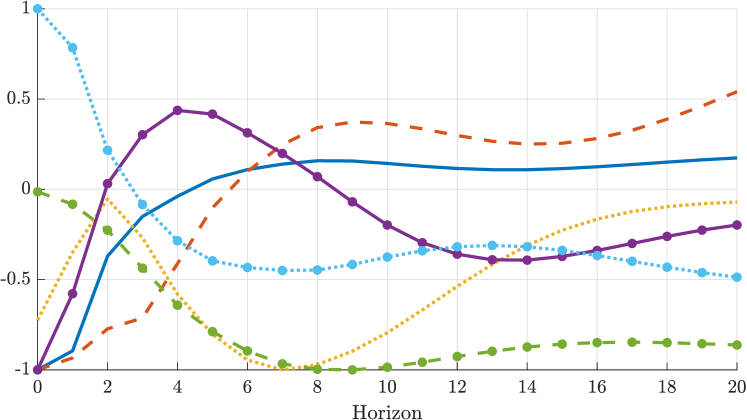
Figure 1: Selected impulse responses of macro observables to monetary and fiscal policy shocks. Here the impulse response functions are normalized to have a maximum value of $1$ or $-1$.

Finally, the true impulse response estimands exhibit a wide variety of shapes. Table 1 shows that the impulse response functions peak at very different horizons and are typically not simple monotonically decaying or even hump-shaped functions: the median number of interior local extrema of the impulse response functions is 2 (a monotonic function would have 0; a hump-shaped function would have 1). Many impulse response functions change sign at some horizon, as evidenced by the average response (across horizons) typically being much smaller than the maximal response. Finally, the smoothness of the impulse response functions varies substantially: the R-squared value in a regression of the impulse responses $\{\theta_{h}\}_{h=0}^{20}$ on a quadratic polynomial $b_{0}+b_{1}\times h+b_{2}\times h^{2}$ has 10th and 90th percentiles given by 0.46 and 0.98, respectively. For further illustration, Figure 1 displays the true values of six impulse response functions, providing a representative picture of the heterogeneity. The figure illustrates that, while some impulse response functions approximately return to 0 at long horizons, many do not, and some have the largest response even beyond horizon $h=20$.

4 Estimation methods

We now give a brief overview of the different VAR- and LP-based estimation methods that we consider in the simulation study. Though all these methods aim at estimating the same population impulse responses defined in Section 3.2, they differ in terms of their bias-variance properties, and in terms of their robustness to non-invertibility. Further implementation details are relegated to Appendix B. All estimators include an intercept.

Local projection approaches.

The basic idea behind local projections, as proposed by Jordà (2005), is to estimate the impulse responses separately at each horizon by a direct regression of the future outcome on current covariates. We consider three such approaches:

1. Least-squares LP. OLS regression of the response variable $y_{t+h}$ on some innovation variable $x_{t}$, controlling for $p$ lags of all data series $w_{t}$. The innovation variable equals $x_{t}=\varepsilon_{1,t}$ for “observed shock” identification. For recursive identification, $x_{t}$ equals the policy variable $i_{t}$, and we additionally control for the contemporaneous values of the variables that are ordered before $i_{t}$ in the system (Plagborg-Møller & Wolf, 2021). For IV identification, we set $x_{t}=i_{t}$ and instrument for this variable using the IV $z_{t}$ (this is the LP-IV estimator of Stock & Watson, 2018). Since least-squares LP does not mechanically impose any functional form on the relationship between impulse responses at different horizons $h$, it does not suffer from extrapolation bias. However, these estimated impulse response functions tend to look jagged in finite samples and be estimated with high variance at longer horizons.

2. Bias-corrected LP (abbreviated “BC LP”). Herbst & Johannsen (2023) propose a bias-corrected version of LP, which partially removes the bias that is due to high persistence in the data. Though this bias is theoretically of order $T^{-1}$ (where $T$ is the sample size) and thus asymptotically negligible relative to the standard deviation, Herbst & Johannsen demonstrate that the bias can be sizable in sample sizes typical in the applied macroeconometrics literature.

3. Penalized LP (abbreviated “Pen LP”). To lower the variance of least-squares LP at the expense of potentially increasing the bias, Barnichon & Brownlees (2019) propose a penalized regression modification of LP. The estimator minimizes the sum of squared forecast residuals (across both horizons and time) plus a penalty term that encourages the estimation of smooth impulse responses. This is a type of shrinkage estimation: the unrestricted least-squares estimate is pushed in the direction of a smooth quadratic function of the horizon. The degree of shrinkage is chosen by cross-validation.

VAR approaches.

Like local projections, a VAR with lag length $p$ flexibly estimates the impulse responses out to horizon $p$; however, the VAR extrapolates the responses at longer horizons $h>p$ using only the sample autocovariances out to lag $p$. As suggested by the analysis in Section 2, this tends to generate impulse response estimates with lower variance but higher bias than LP estimates at intermediate and long horizons. We consider four such VAR-based approaches:

1. Least-squares VAR. Standard VAR impulse response estimates based on equation-by-equation OLS estimates of the reduced-form coefficients.

2. Bias-corrected VAR (abbreviated “BC VAR”). As above, but follows Kilian (1998) in using the formula in Pope (1990) to analytically correct the order-$T^{-1}$ bias of the reduced-form coefficients caused by persistent data.

3. Bayesian VAR (abbreviated “BVAR”). As above, but where the reduced-form coefficients are estimated from a Bayesian VAR with automatic prior selection as in Giannone et al. (2015). We report the posterior means of the impulse responses calculated from 100 draws. The prior specification follows the popular Minnesota prior, but with modifications that allow for cointegration. The prior variance hyper-parameters (and thus the degree of shrinkage) are chosen in a data-dependent way by maximizing the marginal likelihood.

4. VAR model averaging (abbreviated “VAR Avg”). Hansen (2016) develops a data-driven method for averaging across the impulse response estimates produced by several different VAR specifications. We construct a weighted average of 40 different specifications, each of which is estimated by OLS: univariate AR(1) to AR(20) models, and multivariate VAR(1) to VAR(20) models. The weights are chosen to minimize an empirical estimate of the final impulse response estimator’s MSE.

   The VAR model averaging estimator effectively includes LP among the list of candidate estimators (as in the related approach of Miranda-Agrippino & Ricco, 2021). This is because the candidate VAR(20) model gives results similar to LP with several lagged controls, at all horizons considered in our study (Plagborg-Møller & Wolf, 2021).

Observed shock identification is carried out by simply ordering the shock first in the recursive VAR. Recursive identification is implemented as usual in the VAR literature. We consider two different approaches to IV estimation:

1. Internal instruments. Proceed as if the IV were equal to the true shock of interest, i.e., order the IV first in the VAR and compute responses to the first orthogonalized innovation (Ramey, 2011). Plagborg-Møller & Wolf (2021) prove that this approach consistently estimates the normalized structural impulse responses (10) even if the IV is contaminated with measurement error as in (9), and even if the shock is non-invertible.

2. SVAR-IV (also known as proxy-SVAR). Exclude the IV from the reduced-form VAR, and estimate the structural shock by projecting the IV on the reduced-form VAR innovations (Stock, 2008; Stock & Watson, 2012; Mertens & Ravn, 2013; Gertler & Karadi, 2015). This estimator is consistent if the shock of interest is invertible, but not otherwise (Forni et al., 2019; Plagborg-Møller & Wolf, 2022; Miranda-Agrippino & Ricco, 2023). We shall see that the SVAR-IV estimator tends to exhibit lower dispersion than the “internal instruments” estimator due to the smaller dimension of the VAR system.

We implement the “internal instruments” approach using all four types of VAR estimation techniques described earlier. For brevity, we only consider the least-squares version of the “external instrument” SVAR-IV estimator.

Lag length selection.

As a baseline, the LP and VAR estimators use $p=4$ lags for estimation (except of course VAR model averaging, which uses many different lag lengths). In our DGPs, the Akaike Information Criterion almost always selects very short lag lengths $\hat{p}_{AIC}$, as we discuss further in Section 5.6 below. Thus, for all intents and purposes, our results may be interpreted as having been generated by the lag length selection rule $p=\max\{\hat{p}_{AIC},4\}$. Our reading of applied practice is that researchers typically include at least 4 lags in quarterly data. Results for $p=8$ are discussed in Section 5.5.

5 Results

This section presents our simulation results. We summarize the results through four lessons, presented in separate subsections. The first three lessons focus on observed shock identification. The fourth lesson is concerned with IV identification. We show in Section 5.5 that these conclusions are qualitatively robust to several alterations of our baseline simulation specification (including less persistent DGPs and recursive identification). Finally, in Section 5.6, we justify our focus on the average performance of estimators across DGPs, by arguing that there is limited scope for selecting among estimators in a data-dependent way.

Throughout this section we present results for our 6,000 monetary and fiscal policy shock DGPs considered jointly rather than separately. For each DGP, we simulate time series of length $T=200$ quarters and approximate the population bias and variance of the estimators by averaging across 5,000 Monte Carlo simulations. The main results (excluding robustness checks) take about one week to produce in Matlab on a research computing cluster with 300 parallel cores.

5.1 There is a clear bias-variance trade-off between LP and VAR

Our first takeaway is that researchers invariably face a bias-variance trade-off: because most of our DGPs are not well approximated by finite-order VAR models, least-squares LPs tend to have lower bias, while least-squares VAR estimators tend to have lower variance, consistent with the simple analytical example provided in Section 2. Strictly speaking, these statements are only exactly true for the bias-corrected versions of the estimators (Herbst & Johannsen, 2023; Pope, 1990; Kilian, 1998), as the high persistence of our DGPs imparts a sizable finite-sample bias in the estimators at intermediate and long horizons, particularly for LPs. This bias correction, however, is not a free lunch, as it increases variance.

Observed shock: Bias of estimators

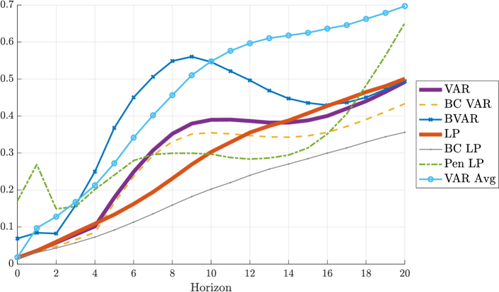
Figure 2: Median (across DGPs) of absolute bias $|E(\hat{\theta}_{h}-\theta_{h})|$ of the different estimation procedures, relative to $\sqrt{\frac{1}{21}\sum_{h=0}^{20}\theta_{h}^{2}}$.

Observed shock: Standard deviation of estimators

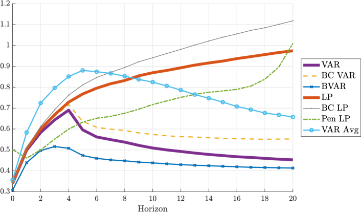
Figure 3: Median (across DGPs) of standard deviation $\sqrt{\operatorname*{Var}(\hat{\theta}_{h})}$ of the different estimation procedures, relative to $\sqrt{\frac{1}{21}\sum_{h=0}^{20}\theta_{h}^{2}}$.

Figures 3 and 3 depict the bias-variance trade-off at various horizons. These figures show the median (across our 6,000 DGPs) of the absolute bias $|E(\hat{\theta}_{h}-\theta_{h})|$ or the standard deviation $\sqrt{\operatorname*{Var}(\hat{\theta}_{h})}$, respectively, as a function of the horizon. The different lines correspond to different estimators $\hat{\theta}_{h}$, with least-squares LP and VAR being the thick lines. Before taking the median, we cancel out the units of the response variables by dividing the bias and standard deviation by $\sqrt{\frac{1}{21}\sum_{h=0}^{20}\theta_{h}^{2}}$, i.e., the root mean squared value of the true impulse response function out to horizon 20. Note that the scale of the vertical axis differs between the bias and standard deviation plots.

The figures show that least-squares LP and VAR estimators have similar bias and variance at horizons $h\leq p=4$, but not at longer horizons $h>p$. The median biases then generally increase with the horizon, with the bias of VAR exceeding that of LP, except at long horizons. While the median standard deviation of LP is increasing in the horizon, that of VAR instead displays a hump-shaped pattern. At long horizons, the median standard deviation of LP is about double that of VAR. These observations are broadly consistent with the asymptotic results in Section 2, Schorfheide (2005), and Plagborg-Møller & Wolf (2021).

Our results also show that the bias correction procedure of Herbst & Johannsen (2023) is critical to achieving uniformly low bias for the LP approach. Though the asymptotic bias of LP is zero when the shock is observed, as discussed in Section 2, the high persistence of our DGPs implies that the small-sample bias of least-squares LP is non-negligible at intermediate and long horizons, especially the latter. The bias-corrected version of LP proposed by Herbst & Johannsen (thin line with small dots in the figures) eliminates about a third of the bias at all horizons. In comparison with the LP case, bias correction is not as critical for VAR estimation, though the bias-corrected VAR estimator (dashed line) does have a somewhat lower bias than the least-squares VAR estimator at long horizons. After bias correction, LP has lower (median) bias than VAR at all horizons, as predicted by asymptotic theory. We further show in Section 5.5 below that such bias correction is not nearly as important in less persistent, stationary DGPs.

Observed shock: Least-squares LP vs. Bias-Corrected LP

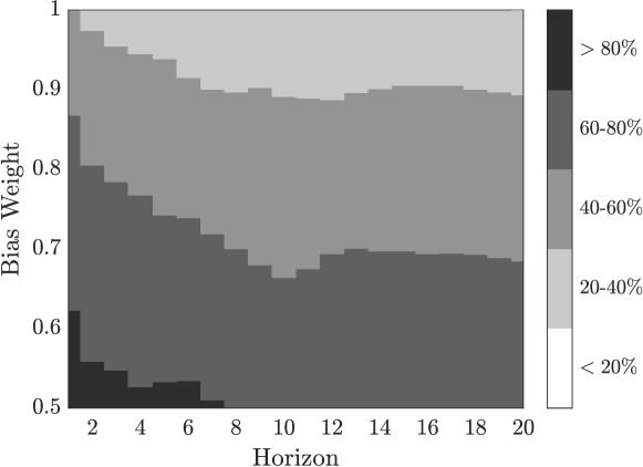
Figure 4: Fraction of DGPs for which the least-squares LP estimator has a lower loss than bias-corrected LP. The darker the region, the higher the fraction of DGPs for which least-squares LP is preferred. Horizontal axis: impulse response horizon $h$. Vertical axis: weight $\omega$ on squared bias in the loss function (4). The loss function is normalized by the scale of the true impulse response function, as in Figures 3 and 3. The impact horizon $h=0$ is omitted due to numerical equivalence between the estimators.

Observed shock: Least-squares VAR vs. Bias-Corrected VAR

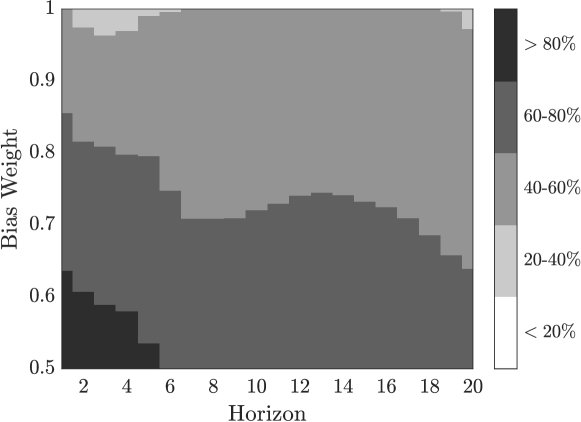
Figure 5: Fraction of DGPs for which the least-squares VAR estimator has a lower loss than the bias-corrected VAR estimator. The darker the region, the higher the fraction of DGPs for which least-squares VAR is preferred. See caption for Figure 5. The impact horizon $h=0$ is omitted due to numerical equivalence between the estimators.

Bias correction is not a free lunch, however, as it is associated with a substantial increase in variance. Figure 3 shows that the bias-corrected LP and VAR estimators have uniformly higher median standard deviation than the uncorrected estimators. In fact, bias-corrected LP has not only the uniformly lowest median bias among the methods we consider, it also has the uniformly highest standard deviation. Figures 5 and 5 show head-to-head comparisons of the least-squares and bias-corrected estimators for the LP and VAR cases, respectively. The figures show the fraction of DGPs for which the least-squares estimator achieves a lower loss (4) than the bias-corrected estimator, as a function of the horizon $h$ and the weight $\omega$ attached to squared bias in the loss function; to interpret the figures, recall that $\omega=0.5$ corresponds to MSE loss, while $\omega=1$ corresponds to an exclusive focus on bias at the expense of variance. The darker the plot, the more often is the least-squares estimator preferred over the bias-corrected one. Evidently, one has to attach a very high weight $\omega$ to bias in the loss function to prefer the bias-corrected estimator in more than 60% of DGPs; furthermore, a researcher with MSE loss would usually prefer the uncorrected estimators.

5.2 Bias-corrected LP is the best estimator if and only if the researcher overwhelmingly prioritizes bias

Our second takeaway is that bias-corrected LP is the single best estimator in our choice set if and only if the researcher’s loss function overwhelmingly prioritizes bias. In contrast, uncorrected LP is never the best option if the goal is to minimize average loss across our DGPs. Under MSE loss, penalized LP typically outperforms the other LP procedures as it has substantially lower variance, though at the expense of a moderate increase in bias.

Observed shock: Optimal estimation method

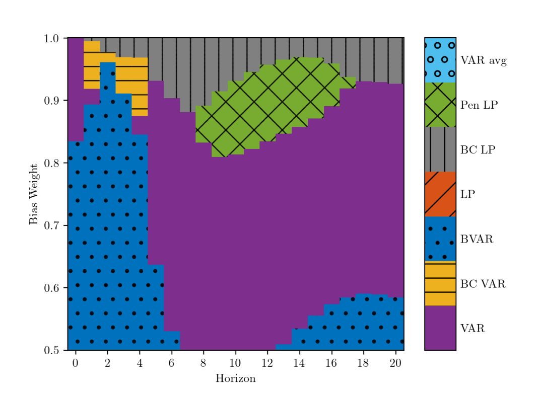
Figure 6: Method that minimizes the average (across DGPs) loss function (4). Horizontal axis: impulse response horizon. Vertical axis: weight on squared bias in loss function. The loss function is normalized by the scale of the impulse response function, as in Figures 3 and 3. At $h=0$, VAR and LP are numerically identical; we break the tie in favor of VAR.

Figure 6 shows the optimal estimation method as a function of the horizon $h$ and the bias weight $\omega$. The colors and patterns indicate the estimation method that minimizes the average loss (4) across DGPs, after normalizing the loss to cancel out units as in Figures 3 and 3. In this subsection we focus on the top part of Figure 6, i.e., where the weight $\omega$ on bias in the loss function is high. Bias-corrected LP emerges as the best estimator at most horizons in this case, as is to be expected given its excellent bias properties in Figure 3; nevertheless, the figure shows that the optimality of bias-corrected LP is predicated on $\omega$ exceeding roughly 0.9, or even higher at some horizons, corresponding to an overwhelming focus on minimizing bias rather than variance. In contrast, uncorrected least-squares LP is essentially dominated: it has greater bias than bias-corrected LP (notably at longer horizons), yet materially higher variance than least-squares VAR or other shrinkage methods, and so no part of Figure 6 is orange with diagonal lines. We discuss the rest of Figure 6 in the next subsection.

Observed shock: Bias-corrected LP vs. Bias-corrected VAR

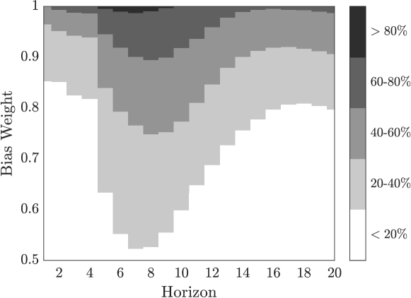
Figure 7: Fraction of DGPs for which the bias-corrected LP estimator has a lower loss than bias-corrected VAR. The darker the region, the higher the fraction of DGPs for which bias-corrected LP is preferred. Horizontal axis: impulse response horizon $h$. Vertical axis: weight $\omega$ on squared bias in the loss function (4). The loss function is normalized by the scale of the true impulse response function, as in Figures 3 and 3. The impact horizon $h=0$ is omitted due to numerical equivalence between the estimators.

Observed shock: Bias-corrected LP vs. Penalized LP

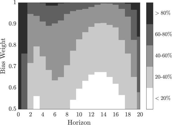
Figure 8: Fraction of DGPs for which the bias-corrected LP estimator has a lower loss than the penalized LP estimator. The darker the region, the higher the fraction of DGPs for which bias-corrected LP is preferred. See caption for Figure 5.

Figures 8 and 8 compare bias-corrected LP to bias-corrected VAR and to penalized LP, respectively. The former figure shows that bias-corrected LP is only preferred to bias-corrected VAR in at least 60% of DGPs when $\omega\geq 0.9$. In the latter figure, we see that the smoothing of impulse responses across horizons that the penalized LP estimator performs is usually attractive whenever $\omega\leq 0.9$, except at very short and very long horizons. By “betting on smoothness”, penalized LP achieves a substantial variance reduction relative to the un-penalized LP procedures, at the expense of a moderate increase in bias, see Figures 3 and 3. In fact, there is a region of Figure 6 with intermediate horizons and moderately high weight on bias where penalized LP (green with diagonal cross-hatching) is the single best estimator. These findings underscore our conclusion that, across the majority of the DGPs, the use of bias-corrected LP can only be justified by committing to a nearly exclusive focus on minimizing bias, with little regard for precision.

5.3 VARs are attractive if there is some concern for precision

Our third takeaway is that VAR estimators are attractive to researchers who place at least moderate weight on variance in their loss function. But the choice of VAR method depends on the horizon: Bayesian VARs perform well at short horizons, least-squares VARs at intermediate horizons, and at long horizons the two are comparable. VAR model averaging, on the other hand, performs poorly regardless of bias-variance preferences.

Returning to Figure 6, we see that for bias weights $\omega$ below 0.9, the optimal estimation method is almost always either least-squares VAR (purple areas) or BVAR (solid-dotted blue). The key attractive property of BVAR is that it has the lowest (median) standard deviation at all horizons among the methods we consider, as seen in Figure 3, though it also has high bias relative to least-squares VAR at intermediate horizons, as shown in Figure 3. The relatively high bias at intermediate horizons is possibly due to the fact that its prior specification, which is conventional in the literature, is motivated by one-step-ahead and long-run forecasting properties, as opposed to medium-run properties.

Observed shock: Least-squares VAR vs. Bayesian VAR

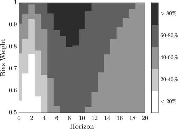
Figure 9: Fraction of DGPs for which the least-squares VAR estimator has a lower loss than the BVAR estimator. The darker the region, the higher the fraction of DGPs for which least-squares VAR is preferred. See caption for Figure 5.

Figure 9 shows that the head-to-head performance of least-squares VAR vs. Bayesian VAR depends on the horizon. At short horizons $h\leq 4$, BVAR is preferred in the majority of DGPs, and indeed it is the overall best estimator for most loss functions that place non-trivial weight on variance (see Figure 6). However, at intermediate horizons $h\in[5,12]$, least-squares VAR is preferred over BVAR in the clear majority of DGPs for most loss functions, and the former estimator is the overall preferred method for loss functions with $\omega\leq 0.8$. At long horizons $h\geq 13$, the two VAR methods are comparable and outperform all other methods, unless the weight on bias in the loss function is high.

Finally, we remark that bias-corrected VAR and VAR model averaging are rarely, if ever, optimal. Bias-corrected VAR (yellow with horizontal lines in Figure 6) can be rationalized at short horizons if the concern for bias is high, but the difference compared to least-squares VAR is small at these horizons, as discussed in Section 5.2. VAR model averaging performs poorly regardless of loss function and horizon, as it has substantial bias as well as a high standard deviation relative to other VAR-based estimators (see Figures 3 and 3). Closer inspection reveals that the high standard deviation is a consequence of a very fat-tailed sampling distribution, with a non-negligible probability of erratic estimates.

5.4 SVAR-IV is heavily biased, but has relatively low dispersion

Our last takeaway is concerned with IV/proxy identification. Among the invertibility-robust “internal instruments” estimators, the bias-variance trade-off is very similar to that already discussed above for the case of an observed shock. The alternative “external instruments” SVAR-IV procedure, however, contributes starkly to the trade-off: it can be severely biased due to its lack of robustness to non-invertibility, but at the same time it also has substantially lower dispersion than the “internal instruments” procedures.

Since first and second moments of IV estimators may not exist theoretically (Sawa, 1972), we in this subsection report median bias (i.e., in each DGP, the median of the estimation error) instead of (mean) bias, and the interquartile range instead of the standard deviation. We refer to the latter as “dispersion.”

IV: Median bias of estimators

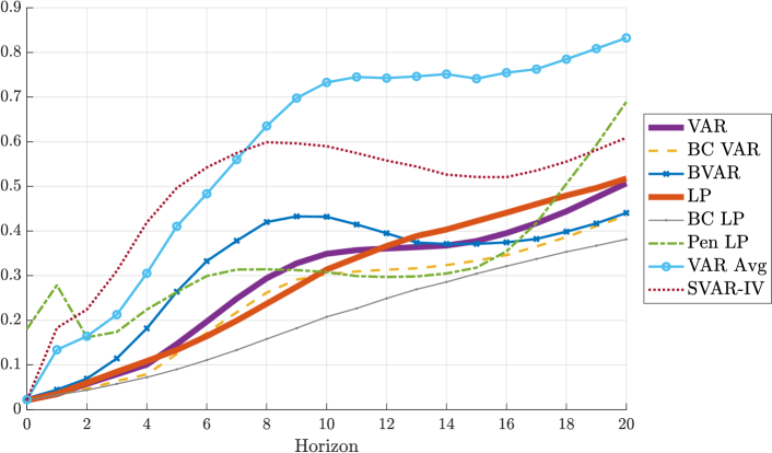
Figure 10: Median (across DGPs) of absolute median bias of the different estimation procedures, relative to $\sqrt{\frac{1}{21}\sum_{h=0}^{20}\theta_{h}^{2}}$. The first seven estimators listed in the figure legend include the proxy/IV directly in the observed data vector, see Section 4.

IV: Interquartile range of estimators

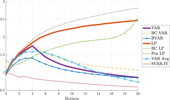
Figure 11: Median (across DGPs) of interquartile range of the different estimation procedures, relative to $\sqrt{\frac{1}{21}\sum_{h=0}^{20}\theta_{h}^{2}}$. See caption for Figure 11.

Figures 11 and 11 show the median bias and interquartile range of the various IV estimators. If we ignore the dotted line representing SVAR-IV, these figures are qualitatively similar to those presented in Section 5.1. However, SVAR-IV stands out by exhibiting especially high median bias and especially low interquartile range at all horizons. This is consistent with the existing theoretical work referenced in Section 4: unlike the “internal instruments” procedures, SVAR-IV is asymptotically biased when the shock is not invertible, and we saw in Section 3.4 that the degree of invertibility is generally low in our DGPs. On the other hand, the SVAR-IV procedure has fewer parameters to estimate (as it excludes the IV $z_{t}$ from the reduced-form VAR regression), causing a reduction in dispersion relative to the other procedures. Though we view the high median bias of SVAR-IV across our DGPs as worrying, its low dispersion is intriguing and may in some cases trump the bias concerns.

5.5 Robustness

This section argues that our main conclusions in Sections 5.1, 5.2, 5.3 and 5.4 are robust to several alterations of our baseline simulation specification. We pay particular attention to an exercise that replaces our non-stationary encompassing DFM with a stationary version. Various other robustness checks are listed subsequently, with details relegated to LABEL:app:results.

Stationary DGPs.

While the majority of applied papers estimate VARs and LPs with a mix of non-stationary and stationary variables in levels (e.g., Ramey, 2016), in some cases researchers transform all their data to stationarity prior to the analysis. To cover such applications, we have repeated our analysis using the stationary estimated DFM of Stock & Watson (2016) as our encompassing model. We construct impulse response estimands as before and compare the performance of the same estimation methods, except that the BVAR estimator uses a prior that shrinks towards white noise rather than random walks. Details on the implementation and results are presented in LABEL:app:results_stationary.

Our headline qualitative conclusions go through in the stationary DGPs. We observe the same bias-variance trade-off as in our main analysis, with LPs achieving lower bias than VARs at the cost of elevated variance. As a result, except for researchers that exclusively prioritize bias, least-squares VARs or some kind of shrinkage—in the form of Bayesian VARs or penalized LPs—are preferred. The two most notable differences from our baseline analysis are that (i) penalized LP outperforms BVAR for MSE loss at very short horizons, and (ii) due to the moderate persistence of the stationary DGPs, bias correction has less bite, and uncorrected least-squares LP has near-zero bias at all horizons.

Other robustness checks.

The following modifications to our baseline simulation specification all leave our main conclusions qualitatively unchanged.

• Recursive identification: To complement the earlier results with observed shocks and proxy identification, we also consider recursive (Cholesky) identification schemes. We sidestep the controversial issue of whether recursive identification is an economically valid identification strategy by taking as the parameter of interest the shared large-sample limit of the recursive LP/VAR estimators (as the lag length tends to infinity). Details on the definition and empirical implementation are provided in LABEL:app:recursive. Simulation results for recursively identified shocks are similar to those for observed shock identification when the weight $\omega$ on (squared) bias in the loss function exceeds 0.8. However, when $\omega\leq 0.8$, BVAR is more attractive than in our baseline analysis. This is because recursive (i.e., Cholesky) identification relies heavily on estimation of the reduced-form innovation variance-covariance matrix. Uniquely among the estimation procedures we consider, BVAR imposes useful shrinkage on this matrix through the prior. See LABEL:app:results_recursive.

• Salient observables: Our results remain essentially unchanged if we restrict attention to a subset of 17 oft-used, salient macroeconomic time series out of the 207 ones in the full Stock & Watson (2016) data set. We consider the exhaustive list of all 1,581 five-variable DGPs that can be formed from these 17 series, subject to the selection rules in Section 3.3. See LABEL:app:results_salientobs.

• Near-worst-case performance: Whereas our baseline results pertain to the median performance of estimators across DGPs, some researchers may instead prefer to focus on ensuring acceptable performance for particularly challenging DGPs. To this end, LABEL:app:results_losspcntl reports the 90th percentiles of the bias and standard deviation across DGPs. Interestingly, adopting this “near-worst-case” perspective does not alter much the relative magnitudes of bias and standard deviation across estimation procedures. Hence, none of the estimation procedures seem to have a particular advantage in ensuring robustness to challenging environments, over and above their performance in typical DGPs.

• Monetary vs. fiscal shocks: If we consider the monetary shock DGPs separately from the fiscal shock DGPs, then the bias-variance trade-off is almost identical to that when we consider the DGPs jointly. See LABEL:app:results_fiscal_monetary.

• Larger lag length: If the lag length $p$ is set to 8 instead of 4, then LP and VAR are approximately equivalent out to horizon 8, as predicted by asymptotic theory. BVAR is relatively more attractive than in the $p=4$ case, as the prior reduces the effective dimensionality of the otherwise high-dimensional VAR system. Beyond that our conclusions on the overall nature of the bias-variance trade-off are unaffected. See LABEL:app:results_lag.

• Smaller sample size: Halving the sample size to $T=100$ quarters tends to increase the estimator standard deviations more than the biases, so shrinkage techniques look even more desirable than in our baseline, including in particular BVAR. Conversely, for bias-corrected LP to be optimal, bias needs to be prioritized even more heavily. See LABEL:app:results_smallsample.

• Larger sample size and lag length: We set sample size $T=720$ and lag length $p=12$, a configuration reminiscent of monthly data. However, we caution that the set-up does not faithfully represent actual monthly data sets, since our DFM parameters remain fixed at the quarterly calibration described in Section 3. As expected, least-squares LP and VAR have approximately equivalent properties out to horizon 12, while the trade-off between estimators at longer horizons is qualitatively similar to our baseline. At horizons below 12, shrinkage via BVAR or penalized LP is even more attractive than in our baseline, unless the bias weight in the loss function is high. See LABEL:app:results_large.

• More observables: If we increase the number of observed macro variables per DGP from 5 to 7, our conclusions are not affected. The only notable quantitative change is that, for IV identification, SVAR-IV has slightly smaller bias relative to the internal instruments procedures, due to the mechanical increase in the degree of invertibility. See LABEL:app:results_more.

• Variable categories: We find little evidence that the biases or standard deviations of individual impulse response estimators depend systematically on which categories of time series are included in the DGP (e.g., how many real activity or price series are used). See LABEL:app:results_cat.

5.6 Discussion: can we select the estimator based on the data?

It is natural to ask whether, instead of selecting estimators based on average performance across DGPs, the choice of estimator can be guided by the data at hand in each given DGP. We now show that this appears to be difficult, as conventional model selection or evaluation criteria are unable to detect even substantial mis-specification of the VAR(4) model in the vast majority of our DGPs. These findings are consistent with the previously documented poor performance of the VAR model averaging estimator. For simplicity, we focus here on observed shock identification.

First, the Akaike Information Criterion tends to select very short lag lengths $\hat{p}_{AIC}$ in our DGPs, as already mentioned earlier. The 90th percentile of $\hat{p}_{AIC}$ (across simulations) does not exceed 2 in any of our 6,000 DGPs, and it in fact equals 2 in only 68.3% of those DGPs. This frequently used model selection tool therefore essentially never indicates that the VAR(4) specification is mis-specified.

Second, the Lagrange Multiplier test of residual serial correlation has low power in most of our DGPs. We carry out this test by regressing the sample VAR residuals on their first lags, controlling for four lags of the observed variables, and employing the likelihood ratio test defined in Johansen (1995). Using a 10% significance level for the test, only around 8% of the DGPs exhibit a rejection probability above 25%, and none of the DGPs have a rejection probability above 50%. Hence, this conventional specification test of the VAR(4) model is under-powered, despite the fact that many of our DGPs are in fact not well approximated by a VAR(4) model in population, as shown in Section 3.4.

It is of course possible that other model selection criteria or specification tests will work better. However, at a minimum, the performance of the VAR model averaging estimator discussed in Section 5.3 and the evidence presented in this subsection together suggest that it is not straightforward to develop effective data-dependent estimator selection rules for use on conventional macroeconomic time series data.

6 Conclusion and directions for future research

We conducted a large-scale simulation study of the performance of LP and VAR structural impulse response estimators, as well as several variants of these methods. We drew the following four main conclusions.

1. As predicted by theory, there is a non-trivial bias-variance trade-off between least-squares LP and VAR estimators (after bias correction). Empirically relevant DGPs are unlikely to admit exact finite-order VAR representations, and so mis-specification of VAR estimators is indeed a valid concern, as discussed by Ramey (2016) and Nakamura & Steinsson (2018), among others. Nevertheless, the slope of the trade-off is steep, with the lower bias of LP coming at the cost of substantially higher variance.

2. Bias-corrected LP is the preferred estimator if and only if the researcher overwhelmingly prioritizes minimizing bias, with little regard to precision. Researchers who use LP should acknowledge their focus on bias, and they should apply the Herbst & Johannsen (2023) bias correction procedure when the data are persistent.

3. For researchers that attach at least moderate weight to variance in their loss function (such as under the conventional MSE criterion), VAR methods are attractive. Specifically, Bayesian VARs perform well at short horizons, least-squares VARs at intermediate horizons, and the two methods are comparable at long horizons. The fact that no single VAR method dominates at all horizons means that researchers must take a stand not only on their preferences for bias and variance, but also on their primary horizons of interest, or alternatively ensure that their findings are supported by multiple procedures.

4. In the case of IV identification, the popular SVAR-IV (or proxy-SVAR) procedure can be severely biased, but it has substantially lower dispersion at all horizons than “internal instruments” procedures such as LP-IV or internal-IV VARs. The high (median) bias of SVAR-IV is due to its lack of robustness to non-invertibility, which is a pervasive and realistic feature of our DGPs.

These conclusions inevitably depend on the choice of encompassing model and the specific implementation of the impulse response estimators. Our paper first and foremost has aimed to bring the bias-variance trade-off in impulse response estimation to the attention of applied researchers. Our particular quantification of this trade-off has sought to capture the wide range of applied settings faced by macroeconomists, by fitting a dynamic factor model with rich short-run and long-run dynamics to the well-known Stock & Watson (2016) data set. Our online code repository (see Footnote 4) facilitates experimentation with alternative encompassing models or estimation procedures.

Our findings point to several potential areas for future research. First, we conjecture that the bias-variance trade-off may differ quantitatively in panel data settings, to the extent that the availability of a large cross section reduces the sampling variance of the estimators for a given time dimension, thus potentially making LP relatively more attractive than in the pure time series case. Second, our analysis has focused on the average performance of estimators across DGPs because we find that conventional model selection or evaluation tools are unable to detect substantial mis-specification of low-order VARs in our simulations; nevertheless, we view data-dependent estimator selection as an area ripe for further investigation. Third, it may be worth investigating whether the performance of the Bayesian VAR procedure at intermediate horizons can be improved by developing alternative prior specifications that are specifically aimed at structural impulse response estimation rather than forecasting, unlike the priors used in much of the literature. Fourth, for the case of IV/proxy identification, an interesting question is whether it is possible to develop alternative invertibility-robust estimation procedures that capture some of the variance improvement enjoyed by the non-robust SVAR-IV estimator. Fifth, we leave exploration of other structural shock identification schemes—such as sign restrictions, long-run restrictions, and non-recursive short-run restrictions—to future work. Sixth, while our simulations were calibrated to quarterly data, it would be illuminating to see whether our conclusions apply also to monthly calibrations.

Appendix A Details on DGP definitions

A.1 Shock definition

Our definition of the structural shock of interest, $\varepsilon_{1,t}$, ensures that it has the largest possible contemporaneous effect on nominal interest rates (for monetary shocks) and government spending (for fiscal shocks). Letting $\eta_{t}\equiv H\varepsilon_{t}$, $\Sigma_{\eta}\equiv\operatorname*{Var}(\eta_{t})$, and $\iota^{*}$ denote the index of the policy instrument $i_{t}$ in the vector $X_{t}$, the shock is thus defined through the solution of the following problem:

$$\max_{H}\quad\Lambda_{\iota^{*},\bullet}He_{1}\quad\text{s.t.}\quad HH^{\prime}=\Sigma_{\eta},$$

where $e_{1}$ selects the first column of $H$. The solution equals $H_{\bullet,1}=\Sigma_{\eta}\Lambda_{\iota^{*},\bullet}^{\prime}(\Lambda_{\iota^{*},\bullet}\Sigma_{\eta}\Lambda_{\iota^{*},\bullet}^{\prime})^{-1/2}$.

A.2 IV process calibration

We calibrate the innovation noise $\sigma_{\nu}^{2}$ in the IV equation to target population IV first-stage F-statistics between 10 and 30 when $T=200$, consistent with borderline weak to moderately strong identification, as in the majority of applied work. This yields $\sigma_{\nu}\in\{1.1,1.5,2.3\}$. We draw $\rho_{z}$ and $\sigma_{\nu}$ uniformly at random from their two sets.

Appendix B Details on estimation procedures

Least-squares LP.

The least-squares LP estimator of the impulse response at horizon $h$ is based on the coefficient $\hat{\beta}_{h}$ in the $h$-step-ahead OLS regression

$$y_{t+h}=\hat{\mu}_{h}+\hat{\beta}_{h}x_{t}+\hat{\zeta}_{h}q_{t}+\sum_{\ell=1}^{p}\hat{\varphi}_{h,\ell}w_{t-\ell}+\text{residual}_{t,h},$$ (B.1)

that is, we regress on the variable $x_{t}$, with controls given by the vector $q_{t}$ as well as $p$ lags of all of the data $w_{t}$. The estimands of Section 3.2 can now be estimated as follows:

1. Observed shock. We set $x_{t}$ equal to the observed shock $\varepsilon_{1,t}$ and omit the contemporaneous controls $q_{t}$ (we still control for lagged data).

2. IV. We estimate a Two-Stage Least Squares (2SLS) version of (B.1), setting $x_{t}$ equal to the policy variable $i_{t}$, and instrumenting for this variable with the IV $z_{t}$. We omit $q_{t}$ in this specification (but still include lagged controls). This is numerically the same as doing a LP of $y_{t+h}$ on $z_{t}$ (with lagged controls), and dividing this coefficient by the LP coefficient in a regression of $i_{t}$ on $z_{t}$ (with lagged controls), see Stock & Watson (2018) and Plagborg-Møller & Wolf (2021).

3. Recursive identification. $x_{t}=i_{t}$ is the policy variable, while $q_{t}$ are the variables ordered before $i_{t}$ in the identification scheme (Plagborg-Møller & Wolf, 2021).

Bias-corrected LP.

We implement the bias-corrected LP estimator of Herbst & Johannsen (2023), using their approximate analytical bias formula for LP with controls and with population autocovariances substituted with sample analogues. Following their recommendation, we implement an iterative bias correction, where the impulse response estimate at horizon $h$ is bias-corrected using the previously corrected impulse response estimates at horizons $1,2,\dots,h-1$.

Penalized LP.

The Barnichon & Brownlees (2019) estimator lowers the variance of LP by exploiting a prior belief in smoothness of the impulse response function across horizons. Following their preferred implementation, we model the impulse response function using B-spline basis functions. The jaggedness penalty function penalizes deviations from a quadratic function of the horizon $h$. We penalize impulse responses up to horizon 20. The penalty parameter is selected in a data-dependent way using 5-fold cross-validation. We do not penalize the coefficients on the control variables in the LP. When reporting relative impulse responses (10), we divide by the least-squares LP estimate of the impact response of the policy variable $i_{t}$ to the structural shock.

Least-squares VAR.

The least-squares VAR coefficient estimates are obtained through equation-by-equation OLS regressions. We perform a Cholesky decomposition of the forecast error variance-covariance matrix and compute impulse response functions with respect to the orthogonalized shocks. The estimands of Section 3.2 can now be estimated as follows:

1. Observed shock. The shock $\varepsilon_{1,t}$ is ordered first in $w_{t}$, and we compute responses to the first innovation.

2. IV. We initially consider an “internal instruments” approach as in Ramey (2011). That is, we include the IV $z_{t}$ in the data vector $w_{t}$, order the IV first, and compute responses with respect to the first innovation (Plagborg-Møller & Wolf, 2021). The relative impulse response (10) is obtained by dividing by the impact response of the policy variable $i_{t}$.

3. Recursive identification. The ordering of variables in $w_{t}$ equals the ordering of the desired population impulse response estimand (cf. Section 3.2), and we compute responses to the innovation of the policy instrument $i_{t}$.

In contrast to the above internal instruments approach, the SVAR-IV (or “proxy-SVAR”) estimator of Stock (2008) is obtained by computing the reduced-form impulse responses $\hat{\Psi}_{h}$ ($h=0,1,\dots$) corresponding to a VAR in $\bar{w}_{t}$ (i.e., excluding $z_{t}$), and then reporting relative impulse responses (10) corresponding to the absolute structural impulse responses $\hat{\Psi}_{h}\hat{\gamma}$, where $\hat{\gamma}$ is the sample covariance vector of the reduced-form VAR residuals $\hat{u}_{t}$ and the IV $z_{t}$.

Bias-corrected VAR.

We follow Kilian (1998) and consider a modification of the standard least-squares VAR estimator that applies the Pope (1990) analytical bias correction to the reduced-form VAR coefficient matrices. We use Kilian’s procedure for ensuring the largest eigenvalue of the bias-corrected VAR companion matrix does not exceed 1.

Bayesian VAR.

Our BVAR implementation follows the default prior recommendations of Giannone et al. (2015), as implemented in their replication code. The prior is therefore a Minnesota prior, extended with the “sum-of-coefficients” and “dummy-initial-observation” priors to improve long-run forecasts. The degrees of shrinkage provided by each of the three prior components are governed by three prior hyper-parameters, which are selected by maximizing the marginal likelihood. To save on computation time, we do not optimize the hyper-parameter-vector $\psi$ (in their notation), i.e., the diagonal of the scale matrix in the Wishart prior on the innovation variance matrix; instead, these hyper-parameters are fixed at the residual variance estimates from preliminary AR(1) regressions.

VAR model averaging.

Hansen (2016) proposes a data-dependent procedure for averaging across impulse responses estimates produced by a collection of different AR and VAR models with different lag lengths. Let $\hat{\delta}_{h}(r)$ denote the un-normalized, least-squares recursive impulse response estimate at some horizon $h$ for model $r=1,\dots,R$. We estimate $\hat{\delta}_{h}(r)$ from $R=40$ candidate models: first, univariate AR models for $y_{t}$ with lag lengths from $p=1$ up to $p=20$; and second, VAR models in $w_{t}$ with lag lengths from $p=1$ up to $p=20$. As in Hansen (2016), the variance-covariance matrix of innovations $\Sigma$ and thus the impact effect $\delta_{0}$ are fixed across candidate models and treated as known without error. The VAR model averaging estimator is given by $\sum_{r=1}^{R}\hat{\omega}_{r}\hat{\delta}_{h}(r)$, where the weights $\{\hat{\omega}_{r}\}_{r=1}^{R}$ are chosen to minimize the data-dependent approximated MSE estimate $\hat{M}(\omega_{1},\dots,\omega_{R})\approx E[T(\sum_{r=1}^{R}\omega_{r}\hat{\delta}_{h}(r)-\delta_{h})^{2}]$, subject to the constraints that all weights are nonnegative and $\sum_{r=1}^{R}\omega_{r}=1$. Details of the MSE estimate are given in Hansen (2016, Section 6). We run this optimization for the weights separately at each impulse response horizon. Relative impulse responses (10) are computed by dividing the absolute impulse response by the least-squares VAR(4) impact impulse response estimate of $i_{t}$ with respect to the identified shock.

References

- Austin (2020) Austin, B. A. (2020). Essays on Labor Economics and Econometrics. PhD thesis, Harvard University. Chapter 2: “The trade-off between LP-IV and SVAR-IV estimation”.
- Bai & Ng (2004) Bai, J. & Ng, S. (2004). A PANIC Attack on Unit Roots and Cointegration. Econometrica, 72(4), 1127–1177.
- Barigozzi et al. (2021) Barigozzi, M., Lippi, M., & Luciani, M. (2021). Large-dimensional Dynamic Factor Models: Estimation of Impulse–Response Functions with I(1) cointegrated factors. Journal of Econometrics, 221(2), 455–482.
- Barnichon & Brownlees (2019) Barnichon, R. & Brownlees, C. (2019). Impulse Response Estimation by Smooth Local Projections. The Review of Economics and Statistics, 101(3), 522–530.
- Brugnolini (2018) Brugnolini, L. (2018). About Local Projection Impulse Response Function Reliability. CEIS Research Paper, Vol. 16, Issue 6, No. 440.
- Bruns & Lütkepohl (2022) Bruns, M. & Lütkepohl, H. (2022). Comparison of local projection estimators for proxy vector autoregressions. Journal of Economic Dynamics & Control, 134, 1–17.
- Choi & Chudik (2019) Choi, C.-Y. & Chudik, A. (2019). Estimating impulse response functions when the shock series is observed. Economics Letters, 180, 71–75.
- Christiano et al. (1999) Christiano, L., Eichenbaum, M., & Evans, C. (1999). Monetary Policy Shocks: What Have We Learned and to What End? In J. B. Taylor & M. Woodford (Eds.), Handbook of Macroeconomics, volume 1A chapter 2, (pp. 65–148). Elsevier.
- Forni et al. (2019) Forni, M., Gambetti, L., & Sala, L. (2019). Structural VARs and noninvertible macroeconomic models. Journal of Applied Econometrics, 34(2), 221–246.
- Gertler & Karadi (2015) Gertler, M. & Karadi, P. (2015). Monetary Policy Surprises, Credit Costs, and Economic Activity. American Economic Journal: Macroeconomics, 7(1), 44–76.
- Giannone et al. (2015) Giannone, D., Lenza, M., & Primiceri, G. E. (2015). Prior selection for vector autoregressions. Review of Economics and Statistics, 97(2), 436–451.
- Hansen (2016) Hansen, B. E. (2016). Stein Combination Shrinkage for Vector Autoregressions. Manuscript, University of Wisconsin-Madison.
- Herbst & Johannsen (2023) Herbst, E. & Johannsen, B. K. (2023). Bias in Local Projections. Manuscript, Board of Governors of the Federal Reserve.
- Inoue & Kilian (2020) Inoue, A. & Kilian, L. (2020). The uniform validity of impulse response inference in autoregressions. Journal of Econometrics, 215(2), 450–472.
- Johansen (1995) Johansen, S. (1995). Likelihood-Based Inference in Cointegrated Vector Autoregressive Models. Oxford University Press.
- Jordà (2005) Jordà, Ò. (2005). Estimation and Inference of Impulse Responses by Local Projections. American Economic Review, 95(1), 161–182.
- Kilian (1998) Kilian, L. (1998). Small-sample Confidence Intervals for Impulse Response Functions. Review of Economics and Statistics, 80(2), 218–230.
- Kilian & Kim (2011) Kilian, L. & Kim, Y. J. (2011). How Reliable Are Local Projection Estimators of Impulse Responses? Review of Economics and Statistics, 93(4), 1460–1466.
- Kilian & Lütkepohl (2017) Kilian, L. & Lütkepohl, H. (2017). Structural Vector Autoregressive Analysis. Cambridge University Press.
- Lazarus et al. (2018) Lazarus, E., Lewis, D. J., Stock, J. H., & Watson, M. W. (2018). HAR Inference: Recommendations for Practice. Journal of Business & Economic Statistics, 36(4), 541–559.
- Leeper et al. (2013) Leeper, E. M., Walker, T. B., & Yang, S.-C. S. (2013). Fiscal Foresight and Information Flows. Econometrica, 81(3), 1115–1145.
- Li et al. (2022) Li, D., Plagborg-Moller, M., & Wolf, C. K. (2022). Local Projections vs. VARs: Lessons From Thousands of DGPs. National Bureau of Economic Research Working Paper No. 30207.
- Marcellino et al. (2006) Marcellino, M., Stock, J. H., & Watson, M. W. (2006). A comparison of direct and iterated multistep AR methods for forecasting macroeconomic time series. Journal of Econometrics, 135(1–2), 499–526.
- Meier (2005) Meier, A. (2005). How Big is the Bias in Estimated Impulse Responses? A Horse Race between VAR and Local Projection Methods. Manuscript, European University Institute.
- Mertens & Ravn (2013) Mertens, K. & Ravn, M. O. (2013). The Dynamic Effects of Personal and Corporate Income Tax Changes in the United States. American Economic Review, 103(4), 1212–1247.
- Miranda-Agrippino & Ricco (2021) Miranda-Agrippino, S. & Ricco, G. (2021). Bayesian Local Projections. Warwick Economics Research Papers No. 1348.
- Miranda-Agrippino & Ricco (2023) Miranda-Agrippino, S. & Ricco, G. (2023). Identification with External Instruments in Structural VARs. Journal of Monetary Economics, 135, 1–19.
- Montiel Olea & Plagborg-Møller (2021) Montiel Olea, J. L. & Plagborg-Møller, M. (2021). Local Projection Inference Is Simpler and More Robust Than You Think. Econometrica, 89(4), 1789–1823.
- Nakamura & Steinsson (2018) Nakamura, E. & Steinsson, J. (2018). Identification in Macroeconomics. Journal of Economic Perspectives, 32(3), 59–86.