Detecting Hidden Units and Network Size
from Perceptible Dynamics

Abstract

The number of units of a network dynamical system, its size, arguably constitutes its most fundamental property. Many units of a network, however, are typically experimentally inaccessible such that the network size is often unknown. Here we introduce a detection matrix that suitably arranges multiple transient time series from the subset of accessible units to detect network size via matching rank constraints. The proposed method is model-free, applicable across system types and interaction topologies and applies to non-stationary dynamics near fixed points, as well as periodic and chaotic collective motion. Even if only a small minority of units is perceptible and for systems simultaneously exhibiting nonlinearities, heterogeneities and noise, exact size detection is feasible. We illustrate applicability for a paradigmatic class of biochemical reaction networks.

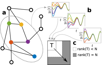
Figure 1: Revealing network size from the dynamics of perceptible units. (a) Scheme of a network of $N$ units where only $n<N$ units (colored disks, encircled by dashed line) are accessible for measurement (perceptible). (b) Transient time series measured from accessible units, started from different initial conditions (trajectory colors match observable units in (a)). (c) Observed nonlinear, multi-dimensional time series are arranged into the detection matrix $T_{k}$, satisfying the condition $\operatorname{rank}\left(T_{k}\right)=N$ if and only if $kn>N$ and $M>N$, according to (6) introduced below.

Networks of interacting dynamical units prevail across natural and human-made systems Strogatz (2001); Newman (2010); Motter and Timme (2018). Examples range from intra-cellular gene-regulatory networks critical for survival Karlebach and Shamir (2008); Huang et al. (2017) to power grids supplying electric energy on demand Filatrella et al. (2008); Rohden et al. (2012); Menck et al. (2013); Motter et al. (2013); Menck et al. (2014); Witthaut et al. (2016) and to social and transportation networks determining how ideas and diseases spread Brockmann and Helbing (2013); Sun et al. (2014); Horváth and Kertész (2014). Key properties of the physical interaction topology in such networks fundamentally underlie their function such that revealing them from measurements of the collective network dynamics constitutes a topical field of research Yeung et al. (2002); Gardner et al. (2003); Yu et al. (2006); Timme (2007); Yu and Parlitz (2011); Shandilya and Timme (2011); Barzel and Barabási (2013); Timme and Casadiego (2014); Han et al. (2015); Casadiego and Timme (2015); Mangan et al. (2016); Casadiego et al. (2017); Nitzan et al. (2017).

However, dynamical data from many networks are often only incompletely accessible, because many of their units are hidden from measurements. Thus the dynamics of a possibly small subset of units might be available only. Such hidden units typically complicate the inference of direct interactions by correlating or decorrelating the dynamics of measured units in unpredictable ways Soudry et al. (2015); Lünsmann et al. (2017). Nevertheless, partial information about a networked system may provide hints about overall features of the network. For instance, approximating the network dynamics via model differential equations may help to detect the existence and location of a single hidden unit through heuristics performed on reconstructed connectivity matrices for different time windows Su et al. (2012); Shen et al. (2014); Su et al. (2016). Other schemes exploit dynamics to determine paths from observed, via hidden, to observed units Gonçalves et al. (2007); Gonçalves and Warnick (2008); Yuan et al. (2011) and typically require to know the exact number of hidden units a priori. Yet, how to reveal the number of many hidden units, or equivalently, the overall network size from time series recorded from the collective dynamics of accessible units remains generally unknown.

Here, we show that measuring the transient collective dynamics of a subset of perceptible network units (accessible to measurement) may robustly reveal the exact number of hidden units and thus identify the network size. We demonstrate how specifically grouping different transient time series obtained from perceptible units into a detection matrix yields bounds relating the rank of such matrix to the size of the full network, see Fig. 1. We propose a simple detection algorithm to exactly find the number of hidden units, even if they are the minority by far. The number of time series necessary to reliably identify network size only linearly scales with network size, thus making size detection scalable. The proposed method generalizes from linear and linearized dynamics near fixed points to dynamics near periodic orbits as well as to collective irregular and chaotic dynamics, without requiring knowledge of a system model. Even for systems simultaneously exhibiting nonlinearities, heterogeneities, and noise detection may be feasible and exact.

Theory of detecting network size from observed dynamics. Consider a network dynamical system

$$\dot{\boldsymbol{z}}=\boldsymbol{F}(\boldsymbol{z}),$$ (1)

of an unknown number $N$ of coupled units $i\in\{1,\ldots,N\}$ where $\boldsymbol{z}(t):=[z(t),z_{2}(t),$ $\ldots,z_{N}(t)]^{\mathsf{T}}\in\mathbb{R}^{N}$ is the system’s state at time $t\in\mathbb{R}$ and $\boldsymbol{F}:\,\mathbb{R}^{N}\rightarrow\mathbb{R}^{N}$ an unknown smooth function that defines its rate of change and thereby the collective network dynamics. For simplicity, we first present the idea of identifying network size for noise-free linear dynamics close to fixed points and below discuss how it generalizes to more complex dynamics, including periodic and aperiodic, irregular dynamics, e.g., noisy and collective chaotic motion. Close to a fixed point $\boldsymbol{z}^{*}$ where $\boldsymbol{F}(\boldsymbol{z}^{*})=0$, a first order approximation of (1) in terms of $\boldsymbol{x}(t)=\boldsymbol{z}(t)-\boldsymbol{z}^{*}$ yields

$$\boldsymbol{\dot{x}}(t)=A\boldsymbol{x}(t)$$ (2)

where $A\in\mathbb{R}^{N\times N}$ with elements $A_{ij}=\partial F_{i}/\partial x_{j}\left(\boldsymbol{z}^{*}\right)$ is the Jacobian matrix of $\boldsymbol{F}$ evaluated at $\boldsymbol{z}^{*}$ and defines an unknown proxy for the connectivity of the system, i.e. $A_{ij}\neq 0$ if unit $j$ directly acts on $i$ and $A_{ij}=0$ otherwise. Solving (2) yields $\boldsymbol{x}(t)=\exp(At)\boldsymbol{x}(0),$ where $\boldsymbol{x}(0)\in\mathbb{R}^{N}$ is a vector of initial conditions at $t=0$ and $\exp(\cdot)$ denotes the matrix exponential function.

How can we uncover network size, i.e. find how many dynamical variables $N$ the system has if we measure the dynamics of only $n<N$ variables? Without loss of generality, we observe the first $n$ components of $\boldsymbol{x}(t)$ and all other $h=N-n$ state variables are hidden from measurement. The time series of measured states $\boldsymbol{y}(t):=\left[x_{1}(t),x_{2}(t),\ldots,x_{n}(t)\right]^{\mathsf{T}}\in\mathbb{R}^{n}$ then satisfy the projection

$$\boldsymbol{y}(t)=\begin{bmatrix}I_{n}&0\end{bmatrix}\boldsymbol{x}(t)=\begin{bmatrix}I_{n}&0\end{bmatrix}\exp(At)\boldsymbol{x}(0),$$ (3)

where $I_{n}$ is the $n\times n$ identity matrix and $0$ represents the $n\times h$ matrix full of zeros. Thus we obtain the constraint

$$y_{i}(t)=\sum\limits_{j=1}^{N}\theta_{ij}(t)x_{j}(0)$$ (4)

for every component $i\in\left\{1,2,\ldots,n\right\}$, where $\theta_{ij}(t)=\left[\exp\left(At\right)\right]{}_{ij}$ is some unknown, time-dependent function and $x_{j}(0)$ is the $j$th component of the initial state, equally unknown for $j\in\{n+1,\ldots,N\}$. Our central question is now: can we find $h=N-n$ despite these many unknowns?

Rewriting the constraint (4) in matrix form yields

$$\boldsymbol{y}^{(m)}(t)=\varTheta(t)\boldsymbol{x}^{(m)}(0),$$ (5)

where $\varTheta(t)\in\mathbb{R}^{n\times N}$ and $\boldsymbol{y}^{(m)}(t)$ is the $m$-th observable trajectory at time $t$ generated from complete initial conditions $\boldsymbol{x}^{(m)}(0)$, different for different $m$. Considering $M$ different trajectories yields a system $Y(t)=\varTheta(t)X_{0},$ where $Y(t):=\left[\boldsymbol{y}^{(1)}(t),\boldsymbol{y}^{(2)}(t),\ldots,\boldsymbol{y}^{(M)}(t)\right]\in\mathbb{R}^{n\times M}$ is the matrix of known dynamical states at time $t$ and the matrix $X_{0}:=\big{[}\boldsymbol{x}^{(1)}(0),\boldsymbol{x}^{(2)}(0),$ $\ldots,\boldsymbol{x}^{(M)}(0)\big{]}\in\mathbb{R}^{N\times M}$ collects different initial conditions. If these trajectories are sampled at $k$ different time points $t_{1},\ldots,t_{k}$, for each trajectory measured relative to its initial time, we group all values of $Y(t)$ evaluated up to time $t_{k}$ into a detection matrix

$$T_{(k,M)}=\Theta_{(k)}X_{0},$$ (6)

where $T_{(k,M)}\left(t_{1},\ldots,t_{k}\right):=\left[Y(t_{1})^{\mathsf{T}},\ldots,Y(t_{k})^{\mathsf{T}}\right]^{\mathsf{T}}\in\mathbb{R}^{kn\times M}$ and $\Theta_{(k)}\left(t_{1},\ldots,t_{k}\right):=\big{[}\varTheta(t_{1})^{\mathsf{T}},$ $\ldots,\varTheta(t_{k})^{\mathsf{T}}\big{]}^{\mathsf{T}}\in\mathbb{R}^{kn\times N}$ . We note that here the lower indices $k,M$ refer to the size ($kn\times M$) of the detection matrix, not to any element of a matrix.

Equation (6) linearly relates the detection matrix $T_{(k,M)}$ assembled from the $M$ different time series sampled at $k$ different times each, to unknown maps $\Theta_{(k)}$ encoding the dynamical evolution (i.e. consequences of the flow of the system) and to the initial conditions $X_{0}$ with also $(N-n)M$ unknown elements. Despite little is known about $\Theta_{(k)}$ and $X_{0}$, the time series merged into the linear system (6) already provide valuable information about the network size $N$. Specifically,

$$\operatorname{rank}\left(T_{(k,M)}\right)\leq\min\left(\operatorname{rank}\left(\Theta_{(k)}\right),\operatorname{rank}\left(X_{0}\right)\right),$$ (7)

and the rank of $T_{(k,M)}$ generically increases with increasing the number $M$ of time series ($\operatorname{rank}(X_{0})=\min\left(N,M\right)$), as well as with increasing the number of sampling points $k$ on each of them, because the rank of $\Theta_{(k)}$ increases ($\operatorname{rank}(\Theta_{(k)})=\min\left(kn,N\right)$), until the rank is maximal and equals $N$. Merging sufficiently many time series, $M>N$, of sufficient length $k>N/n$ we obtain $\operatorname{rank}\left(\Theta_{(k)}\right)=\operatorname{rank}\left(X_{0}\right)=\operatorname{rank}\left(T_{(k,M)}\right)=N$. At this point, adding more time series, i.e. increasing $M$, or extending observations on each of them, i.e. increasing $k$, does not further increase $\operatorname{rank}\left(T_{(k,M)}\right)$ so computing the rank of the detection matrix $T_{(k,M)}$ assembled from time series of the subset of the $n$ measured units yields the network size $N$ via (6). Thus,

$$\hat{h}=\operatorname{rank}\left(T_{(k,M)}\right)-n.$$ (8)

is the estimated number of hidden units. Interestingly, there is no principal lower bound on how small $n$ must be for this relation to hold theoretically. In practice, measurement errors, noise and limits in the detection matrix condition number Stoer and Bulirsch (2013) limit feasible ratios $n/N$, see our analyses below.

Algorithm for detecting network size from time series data. One practical way of inferring network size through the rank inequality (7) is to numerically compute the ordered singular values $\sigma=(\sigma_{1},\ldots,\sigma_{b})$ of $T_{(k,M)}$ such that $\sigma_{1}\geq\sigma_{2}\geq...\geq\sigma_{b}$ , where $b=\min\{kn,M\}$ specifies the number of singular values, and to detect the largest $\Delta_{\mathsf{max}}$ of the gaps

$$\Delta{}_{j}=\log(\sigma_{j})-\log(\sigma_{j+1})$$ (9)

on the logarithmic scale. To safely detect the network size $N$ given a known number $n$ of measured units from iteratively increasing the number of measurements $M$ (see Fig. 1c), we propose the following algorithm:

1. Start, given the lower bound $n\leq N$, with a set of $M=n+1$ measurement trajectories $\boldsymbol{y}^{(m)}(t)$, $m\in\{1,\dots,M\}$.

2. Choose $k=\left\lceil\frac{M}{n}\right\rceil$ different time instants $t_{\kappa}\in\{t_{1},\ldots,t_{k}\}$ separated by $\Delta t=t_{\mathrm{tot}}/k$, where $t_{\mathrm{tot}}$ is the total duration of each time series considered and $t_{1}$ its start time.

3. Construct the detection matrix

   $$T_{(k,M)}=\begin{bmatrix}\boldsymbol{y}^{(1)}(t_{1})&\dots&\boldsymbol{y}^{(M)}(t_{1})\\ \vdots&&\vdots\\ \boldsymbol{y}^{(1)}(t_{k})&\dots&\boldsymbol{y}^{(M)}(t_{k})\end{bmatrix}$$ (10)

   from the measurements $\boldsymbol{y}^{(m)}(t)$ and compute its $b=\min\{kn,M\}=M$ singular values $\sigma\left(T_{(k,M)}\right)$.

4. Compute logarithmic gaps $\Delta{}_{j}$ as in (9).

5. Save the largest gap $\widetilde{N}_{n}^{(M)}:=\max\{\Delta{}_{j}\}$, where $j\geq n$ and $j\not\in\left\{n,2n,\ldots\right\}\cup\{n+1,2n+1,...\},$ avoiding gaps at integer multiples of $n$.

6. To robustly identify size also in case $N$ is such an integer multiple, repeat steps 2–5 for $n-1,...,n-4$ measured units (thus ignoring actually measured units) and take as the estimate

   $$\hat{N}^{(M)}:=\mathrm{median}\{\widetilde{N}_{n}^{(M)}\}.$$ (11)

7. If $\hat{N}^{(M)}$ does not increase further, stop and define $\hat{N}:=\hat{N}^{(M)}$ as an estimate of network size; otherwise, repeat steps 2–6 with one additional measurement, $M\rightarrow M+1$;

Here, step 2 ensures that finally, we will have $kn>N$ because $M>N$, see the examples below.

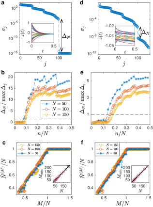
Figure 2: Singular values of detection matrix yield network size. (a) Singular values $\sigma_{j}$ of detection matrix $T_{(k,M)}$ displayed on logarithmic scale for linear networks of $N=100$ diffusively coupled units ($n=30$ measured). The largest gap $\Delta{}_{N}$ reveals the size of the network. Inset: Example trajectories $z_{i}(t).$ (b) Size of $\Delta{}_{N}$ relative to largest $\Delta{}_{j}$ for $j<N$ rises above detection threshold at unity (horizontal dashed line). Every data point corresponds to an average over 20 independent random networks ($M=1.5N$). (c) For increasing number of experiments $M$, the inferred number $\hat{N}^{(M)}$ of units proportionally increases until it stays constant at $\hat{N}^{(M)}=N$ once $M>N$. Inset: Minimum number $M_{\textnormal{min}}$ of experiments to achieve $\hat{N}^{(M)}=N$ for networks of different sizes $N$ (red squares, $n=N/3$ measured units). All results well fit the prediction $M_{\textnormal{min}}=N+1$ (solid line). (d) Gaps revealing network size for Kuramoto oscillators near a phase-locked state ($N=100$, $n=30$ as before). (e) As the theory uses linear approximations, the strength of predictions is weaker for nonlinear systems, but the relative gap size again clearly grows beyond unity (dashed line) with increasing fraction $n/N$ of measured units. (f) Even though $\Delta_{N}$ is smaller compared to the linear dynamics, the same method infers $N$ just as reliably. Here, the prediction is $M_{\textnormal{min}}=N+2$ as one measurement time series is used as a reference. We use homogeneous, directed random graphs with in-degree $g=N/10$ (see Supplement).

Performance of network size detection. To test the predictive power of our theory combined with the simple algorithm provided we inferred the network size for five different classes of network dynamics: (i) noiseless, diffusively coupled one-dimensional linear units collectively converging to stable fixed points, (ii) phase-oscillator networks close to periodic phase-locked states, systems of $N$ three-dimensional coupled oscillatory units that exhibit (iii) regular periodic as well as (iv) irregular chaotic collective dynamics, and (v) noisy, heterogeneous systems with nonlinear dynamics. For settings (i) and (ii), we define the class of diffusively coupled systems of single-variable units via (1) with $F_{i}(\mathbf{z})=\omega_{i}+\sum_{j=1}^{N}A_{ij}f\left(z_{j}-z_{i}\right),$ where $f:\mathbb{R}\rightarrow\mathbb{R}$ is a smooth function and $\omega_{i}\in\mathbb{R}$ is a constant driving signal. We provide all model and simulation details in the Supplement.

For the simplest setting of linear noiseless systems, we take $f(x)=x$ with stable fixed point $\boldsymbol{z}^{*}$ (Fig. 2a-c). The estimated rank of the detection matrix (6) indicated by a pronounced gap in its singular value spectrum accurately predicts network size (Fig. 2a) and is reliable already if only about 10% of the units are measured (Fig. 2b). Measuring larger fractions $n/N$ of units rapidly further improves distinguishing the largest gap $\Delta_{N}$ from other gaps $\Delta_{j}$. For nonlinearly coupled systems of phase-oscillators ($f(x)=\sin(x)$, $\omega_{i}\in[-0.1,0.1]$), performance is similarly high despite locally linear approximations (Fig. 2d-f). We expected this similarity in performance, because phase-locked states map to fixed points in a co-rotating frame of reference and linearization of the sine function constitutes a well-conditioned approximation for $|x|\ll\pi/2$.

Complex transient dynamics and biological networks. The idea introduced above is readily generalized to systems of higher-dimensional units and more complex forms of collective dynamics, including in principle arbitrary periodic or chaotic motion. Now consider that $\boldsymbol{z}^{*}$ is not a fixed point of the dynamics (1) but any point in state space. We locally approximate near $\boldsymbol{z}^{*}$ the nonlinear flow $\boldsymbol{\Phi}_{t}(\cdot)$ Hale and Koçak (2012) defined for all solutions $\boldsymbol{z}(t)$ of the original nonlinear differential equation (1) via $\boldsymbol{z}(t)=\boldsymbol{\Phi}_{t}(\boldsymbol{z}(0))$ from some initial conditions $\boldsymbol{z}(0)$. The difference vector $\delta\boldsymbol{z}(t)=\boldsymbol{z}^{(1)}(t)\boldsymbol{-z}^{(2)}(t)$ of two close-by trajectories indexed $1$ and $2$ then satisfies (see Supplement for a step-by-step derivation)

$$\delta\boldsymbol{z}(t) \doteq D\boldsymbol{\Phi}_{t-t^{*}}\Big{|}_{\boldsymbol{z}^{*}}\delta\boldsymbol{z}(t^{*})$$ (12)

where $D\boldsymbol{\Phi}_{t-t^{*}}\Big{|}_{\boldsymbol{z}^{*}}$ denotes the Jacobian matrix of $\boldsymbol{\Phi}_{t-t^{*}}(\cdot)$ evaluated at $\boldsymbol{z}^{*}$ and the symbol “$\doteq$” indicates first order approximation in the components of $\delta\boldsymbol{z}(t^{*})$. Employing a projection equivalent to (3) above, we now take the time series of the measured units to be

$$\boldsymbol{y}(t)=\begin{bmatrix}I_{n}&0\end{bmatrix}\delta\boldsymbol{z}(t),$$ (13)

the matrix generating the dynamics to have elements

$$\theta_{ij}(t):=\left(D\boldsymbol{\Phi}_{t-t^{*}}\Big{|}_{\boldsymbol{z}^{*}}\right)_{ij}=\frac{\partial\Phi_{i,t-t^{*}}}{\partial z_{j}}\Big{|}_{\boldsymbol{z}^{*}}$$ (14)

and re-obtain (4) for the difference variables. We emphasize that the resulting equations are mathematically identical to (4) such that combining time series data as before into a detection matrix yields the network size exploiting the same principles and steps as above. In simulations, we consider $\boldsymbol{z}^{(2)}(0)=\boldsymbol{z}^{*}$ for simplicity and thus consider $t^{*}=0$ and positive times $t>0$. Figure 3 illustrates successful network size identification for high-dimensional periodic motion and for collective chaotic dynamics.

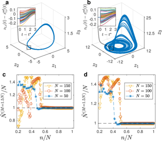
Figure 3: Network size from complex transient dynamics. Projection of sample trajectories of one unit $i$ for (a) periodic and (b) chaotic dynamical regimes. Each time, the system passes a certain region on the attractor (highlighted by dashed square), a random perturbation is applied to the components $z_{1,i}$ (insets). (c,d) Using deviations $\delta z_{i}^{(m)}(t)=z_{1,i}^{(m)}(t-t_{m}^{*})-z_{1,i}^{(1)}(t-t_{1}^{*})$ for each perturbation experiment $m$ to construct $T_{(k,M)}$ reveals the correct system size $\hat{N}^{(M)}=N$, if a sufficient fraction $n/N$ of units is measured. All data points averaged over 20 random network realizations of $N=100$ units with degree ten, exhibiting Rössler oscillatory dynamics, with state $\mathbf{z}_{i}(t)=(z_{1,i}(t),z_{2,i}(t),z_{3,i}(t))$, and diffusive coupling between $\boldsymbol{z}_{2}$-components. In the examples shown, the $z_{1}$-components of units $i$ are perturbed and measured. Despite the coupling being in the $z_{2}$ components, network size identification is accurate at $\hat{N}/N=1$.

To illustrate applicability to biological circuits, we tested networks displaying Michaelis Menten kinetics, a paradigmatic model of biochemical reaction dynamics (see Figure 4 and Supplementary Material). Intriguingly, exact size detection is feasible even in such systems simultaneously exhibiting nonlinearities, heterogeneities and noise. Most interestingly, detection may be exact despite noise. An increasing number of time series taken into account still enables exact size identification, $\hat{N}=N$. See also the Supplement for a systematic evaluation of the influence of noise.

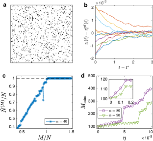
Figure 4: Exact size detection in biological circuits simultaneously exhibiting nonlinearities, heterogeneities, and noise. (a) Adjacency matrix of a coupled Michaelis Menten kinetic network ($N=100$, link weights in grayscale) and (b) its collective noisy dynamics (units of ten randomly selected units displayed, $\eta=10^{-4}$). As for coupled periodic and chaotic systems, deviations $\delta z_{i}^{(m)}(t)=z_{i}^{(m)}(t-t_{m}^{*})-z_{i}^{(1)}(t-t_{1}^{*})$ are used for the reconstruction. (c) Increasing the number $M$ of measurements taken into account in the detection matrix reveals the network size once $M>N$ in the absence of noise. (d) The minimum number $M_{\mathrm{min}}$ of experiments required to obtain an exact size prediction $\hat{N}^{(M)}=N$ for $M\geq M_{\text{min}}$, in dependence of the noise level $\eta>0$.

Discussion and conclusions. In summary, we proposed a theory for determining the network size from time series data sampled from of a potentially small subset of perceptible units. The novel perspective introduced shifts the problem of determining the exact number of hidden units to the task of recording a sufficiently large number of different dynamical trajectories of the perceptible units. It offers a generic tool for detecting the network size or, more generally, the number of independent dynamical variables of multidimensional coupled systems, from a fundamental theorem of linear algebra applied to linear constraints on a suitably constructed detection matrix. The main conditions for applicability are that (i) $M>N$ trials are experimentally feasible and that (ii) the sampling is such that two or more data points on a given trajectory are sufficiently close in state space for the dynamics obtained from local linearization to well approximate the real dynamics. While the time steps $t_{2}-t_{1},\dots,t_{k}-t_{k-1}$ need to be the same in each measurement, we emphasize that only very few such points are needed if not too few nodes are recorded. Network size may be detectable from as few as $k=2$ sample points per trajectory if more than half of all units are perceptible. Moreover, even in modular networks where most perceptible units are located in one module, network size detection may work reliably (see also Supplemental Material at https://doi.org/10.1103/PhysRevLett.122.158301).

Compared to the state of the art, the conditions underlying network size identification can be considered mild, for at least two reasons. First, because so far only one or potentially a few individual hidden nodes are identifiable at all Su et al. (2012); Shen et al. (2014); Su et al. (2016) whereas our approach enables the identification of an extensive number of simultaneously hidden nodes. These may even be the majority of all nodes in the network. Second, because time series analysis methods of finding the attractor dimension (that constitutes a lower bound of and sometimes could equal the dimensionality of state space, and thus the number $N$ of active variables) require $M^{\prime}\gg N$ data points and in addition are typically limited to moderate or even small $N$ of the order of ten or lower Kantz and Schreiber (2004). For example, to obtain faithful attractor dimensions that constitute lower bounds on $N$, as many as $M^{\prime}>10^{4}$ data points may be required for systems with $N=3$ active variables Pecora et al. (2007), whereas our method requires $M^{\prime}=kM$ data points with moderate or small $k\geq 2$ and $M$ just slightly larger than $N$.

We tested the proposed theory employing direct numerical simulations of abstract model systems and generic biological circuit models simultaneously exhibiting three obstacles that may limit network size detection. We find that for successful detection, collective network dynamics may be non-stationary, it may be close to fixed points or more complex such as periodic or possibly aperiodic chaotic or noisy motion. A case study of generic model biological circuits equally reveals network size despite simultaneously exhibiting nonlinearities, heterogeneities and noise. Across these settings, size detection may be exact. The applicability may be limited under conditions where noise strongly dominates the dynamics, only a small fraction of units are perceptible or perceptible units in a modular network are located all in one module. Example studies (see Supplemental Figure S2 for an illustration) suggest that even in the latter extreme setting, although the exact size is not revealed any more, the estimate is still of the same order of magnitude.

A related challenge is network observability Liu et al. (2013); Tang et al. (2014); Whalen et al. (2015); Parlitz (2016), that is to identify a sufficient set of units such that measuring these units’ states reveals the collective state of the entire network. In contrast, our work aims at identifying the number of units in a network, not their states. It is thus conceptually different and exhibits much weaker requirements.

Previous approaches to detect hidden nodes are capable of detecting a single hidden node in an otherwise completely perceptible network: Some Hamilton et al. (2017) employ nonlinear Kalman filters to fit the parameters of a given model and use the covariance matrix of the fitting error; others first approximate the dynamics via differential equations and then determine the existence and location of the hidden unit through heuristic methods Su et al. (2012); Shen et al. (2014); Su et al. (2016). Our theory instead reliably captures many hidden units, is data-driven, relies on sampled time series and thereby requires no model a priori. Furthermore, it provides a mechanistic perspective that not only determines the existence but also reveals the exact number of hidden units. It may thus also complement embedding methods for determining attractor dimension Kantz and Schreiber (2004) that identify the number of active variables from stationary time series, thereby opening up a way to broaden insights about the collective dynamics of multi-dimensional complex systems. Parlitz (2016).