Model Selection for Time Series Forecasting

Abstract

Evaluating predictive models is a crucial task in predictive analytics. This process is especially challenging with time series data where the observations show temporal dependencies. Several studies have analysed how different performance estimation methods compare with each other for approximating the true loss incurred by a given forecasting model. However, these studies do not address how the estimators behave for model selection: the ability to select the best solution among a set of alternatives. In this paper, we address this issue and compare a set of estimation methods for model selection in time series forecasting tasks. We attempt to answer two main questions: (i) how often is the best possible model selected by the estimators; and (ii) what is the performance loss when it does not. Using a case study that comprises 3111 time series we found that the accuracy of the estimators for selecting the best solution is low, despite being significantly better relative to random selection. Moreover, the overall forecasting performance loss associated with the model selection process ranges from 0.28% and 0.58%. We also discovered that the sample size of time series is an important factor in the relative performance of the estimators.

1 Introduction

Estimating the predictive performance of models using the available data is a crucial stage in the data science pipeline. We study this problem for time series forecasting tasks, in which the time dependency among observations poses a challenge to several estimation methods that assume observations are independent.

Performance estimation methods are used to solve two main tasks: (i) to provide a reliable estimate of performance in order to inform the end-user of the expected generalization ability of a given predictive model; and (ii) to use these estimates to perform model selection, i.e., to select a predictive model among a set of possible alternatives that can actually be different parameter settings of the same model. A substantial amount of work addresses the first of these tasks for time series forecasting problems, e.g. bergmeir2012use ; bergmeir2018note ; cerqueira2020evaluating ; tashman2000out ; mozetivc2018evaluate . In this work, we address the second problem. Although similar, model selection and performance estimation are two different problems breiman1992submodel ; arlot2010survey . On the same data set, an estimator may provide the best loss estimations, on average, but not the best model rankings for selection purposes. This idea is illustrated in Figure 1.

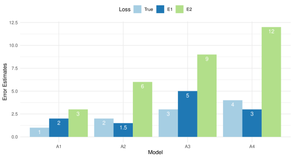
Figure 1: True error (labeled True) and two error estimates (using estimators E1 and E2) of the predictive performance of four models: A1, A2, A3, and A4. The estimator E1 shows, on average, the best estimates. However, E2 produces a perfect ranking of the models contrary to E1.

In this example, there are four predictive models: A1, A2, A3, A4, which are shown in the x-axis of Figure 1. The true test set loss is depicted by the light blue bars. Thus, the correct ranking of the models is A1 $>$ A2 $>$ A3 $>$ A4. A1 is the best model has it shows the lowest test loss. Two estimators, E1 and E2, are used to approximate the error of each model. The estimator E1 produces the best loss approximations (nearest to the true error), on average, relative to estimator E2. However, its estimated ranking (A2 $>$ A1 $>$ A4 $>$ A3) is actually different than the true ranking and worse than the one produced by E2. Despite providing worse performance estimates, E2 outputs a perfect ranking of the models. This example shows that one estimator is better for performance estimation (E1), and the other for model selection (E2). This matter was explored before by Breiman and Spector breiman1992submodel for i.i.d. data sets. They found interesting differences in the relative performance of estimation methods when applied to model selection and performance estimation.

Our goal in this paper is to study the ability of different estimators (e.g. K-fold cross-validation) for model selection in time series forecasting tasks, in which the observations are not i.i.d.. Given a pool of alternative models, we study: (i) how often the best solution is picked (the one which maximizes forecasting performance on test data); and (ii) how much performance is lost when it does not. In other words, we analyse the ability of different estimators to rank the available predictive models by their performance in unseen observations. We are particularly interested in the top ranked model, which is the one most probably selected for deployment, i.e. for predicting future observations of the domain under study.

Most estimation procedures will involve repeating the application of a model to different test sets/folds. The estimation results across these different folds are typically combined using the arithmetic mean. The selected model among a set of considered alternatives is the one with lowest average estimated error. In this paper, we study the possibility of combining the results across folds using the average rank, instead of the average estimated error. The average rank is a non-parametric approach which may be beneficial to smooth the effect of large errors (outliers) in particular folds yang2007consistency .

We carried a set of experiments using 10 estimation methods, 3111 time series data sets, and 50 auto-regressive forecasting models. The results show that the accuracy of the estimators for selecting the most appropriate solution ranges from 7% to 10%. Overall, the forecasting performance loss incurred due to incorrect the model selection ranges from 0.28% to 0.58%. We also controlled the experiments by the sample size of time series and found interesting differences in the relative performance. Particularly, the performance loss is considerably larger for smaller time series. Finally, regarding the strategy for combining the results across folds, we found that the average rank leads to a comparable performance relative to the average error.

In summary, the contribution of this paper is an extensive study comparing a set of performance estimation methods for model selection in time series forecasting tasks. To our knowledge, this paper is the first to quantify the impact of using a particular estimator for model selection in forecasting problems. The experiments carried out in this paper are available online.

This paper is organised as follows. In the next section we review the work related to this paper. In Section 3, we formalise the predictive task relative to time series forecasting and the model selection process. The experiments are presented in Section 4 and discussed in Section 5. Finally, the paper is concluded in Section 6.

2 Related Work

In this section, we provide an overview of the literature related to our work. We briefly describe performance estimation methods designed for time series forecasting models (Section 2.1). We also list previous works which study these methods and highlight our contributions. In Section 2.2, we overview the literature on the application of machine learning methods for forecasting.

2.1 Performance Estimation in Forecasting

Several approaches for evaluating the predictive performance of models in time series have been proposed in the literature. We discuss terminology before describing these. According to Arlot and Celisse arlot2010survey , cross-validation denotes the process of splitting the data, once or multiple times, for estimating the performance of a predictive model. In this process, part of the data is used to fit a model while the remaining observations are used for testing. All methods we analyse in this work follow this procedure. However, we refer to cross-validation as the class of approaches that follow the splitting criteria of K-fold cross-validation and which assume independence among data points. Other procedures, for example prequential dawid1984present , work under different assumptions. Therefore, we designate them accordingly.

Arguably, the most common approach to assess the performance of a forecasting model is a holdout procedure, also known as out-of-sample evaluation (e.g. bergmeir2018note ). The initial part of the time series is used to fit the model, and the last part of the data is used to test it. Tashman tashman2000out recommends applying this approach in multiple testing periods. Indeed, Cerqueira et al. cerqueira2020evaluating show that holdout applied in multiple, randomized, periods leads to the best estimation ability relative to several other state of the art estimators for non-stationary time series.

K-fold cross-validation works by randomly assigning the available observations to K different equally-sized folds. Each fold is then iteratively used for testing a predictive model which is built using the remaining observations. This process is theoretically inadequate to evaluate time series models because the observations are not independent arlot2010survey ; opsomer2001nonparametric . However, Bergmeir et al. bergmeir2012use ; bergmeir2018note show that cross-validation approaches can be successfully applied to estimate the performance of forecasting models. For example, they showed that, in some scenarios, the K-fold cross-validation procedure described above provides better results than out-of-sample evaluation bergmeir2018note . Notwithstanding, several methods have been proposed as extensions to the K-fold cross-validation, which aim at mitigating the problem of the dependence among observations. These include the blocked cross-validation snijders1988cross , modified cross-validation mcquarrie1998regression , and hv-blocked cross-validation racine2000consistent . In different works, both Bergmeir et al. bergmeir2012use and Cerqueira et al. cerqueira2020evaluating compare different estimators for evaluating forecasting models. They suggest using the blocked form of K-fold cross-validation for stationary time series.

The prequential method is also a common evaluation approach for time-dependent data dawid1984present . This method is also referred to as time series cross-validation or time series split by practitioners. Prequential denotes the process in which an observation (or batch of observations) is first used for testing a predictive model and then to update it, and it is the most common solution in data stream mining tasks gama2009evaluating . For more general time series, prequential approaches are typically applied in contiguous blocks of data. Moreover, prequential can be applied in different manners. For example, using a growing window or a sliding window.

The above-mentioned estimation methods are described in more detail in Section 4.4. These have been studied in different works according to how well they approximate the loss that a predictive model incurs in a test set bergmeir2012use ; bergmeir2018note ; cerqueira2020evaluating . The objective was to assess: (i) the magnitude of their estimation errors, and (ii) the direction of the error, i.e., whether the estimators under-estimate or over-estimates the loss of the respective model. These two quantities allow us to analyse which estimators provide the most reliable approximations, on average. They enable the quantification of the generalization ability of models, which help the end-user decide whether or not a model can be deployed. However, as illustrated in Figure 1, the estimator with the best approximations is not necessarily the one presenting the best ranking ability, and thus, the most appropriate for model selection breiman1992submodel . Correctly identifying the relative performance of predictive models is an important feature for model selection. Contrary to related works, we focus on analysing estimation methods from this perspective.

2.2 Machine Learning Methods for Forecasting

Without loss of generality, and as we will describe in Section 4.4, we focus on typical machine learning regression algorithms for forecasting. We apply these in an auto-regressive manner using time-delay embedding, which is formalized in Section 3. In this section, we overview several works which address the applicability of machine learning approaches to forecasting.

Makridakis et al. makridakis2018statistical reported that machine learning approaches performed worse relative to traditional methods such as ARIMA chatfield2000time , exponential smoothing gardner1985exponential , or a simple seasonal random walk. These conclusions were drawn from 1045 monthly time series with low sample size (an average of 118 observations). However, in a more recent work, Makridakis and his colleagues spiliotis2020comparison show that machine learning approaches provide better forecasting performance for SKU demand forecasting when compared to these traditional methods. Moreover, Cerqueira et al. cerqueira2019machine show that the conclusions drawn in makridakis2018statistical are only valid for small time series. In the M5 forecasting competition makridakis2020m5 , the lightgbm gradient boosting method ke2017lightgbm , which is a popular machine learning algorithm, was the method used in the winning solution and some of the runner ups.

Other studies have also shown that standard regression methods can be successfully applied to time series forecasting problems. Cerqueira et al. cerqueira2017dynamic ; cerqueira2019arbitrage develop a dynamic ensemble for forecasting. The ensemble is heterogeneous and comprised by several machine learning methods, along with other traditional forecasting approaches. Corani et al. corani2020automatic propose a method based on Gaussian processes for automatic forecasting. Deep neural networks are increasingly applied to this type of problems and several architectures have been developed, such as N-BEATS oreshkin2019n or DeepAR salinas2020deepar , among others. Another notable work is that by Smyl smyl2020hybrid , which developed a hybrid method which combines a recurrent neural network with exponential smoothing.

3 Problem Definition

In this section, we define two tasks. First, we formalise the time series forecasting problem from an auto-regressive perspective (Section 3.1). Then, we define the model selection problem (Section 3.2). Finally, in Section 3.3 we overview the average rank method for algorithm selection across multiple data sets and how we apply it for model selection within a single data set.

3.1 Auto-regression

Let $Y$ denote a time series $Y=\{y_{1},y_{2},\dots,y_{n}\}$, in which $y_{i}$ is the $i$-th out of $n$ time-ordered observations. The goal is to predict the future values of this time series. Without loss of generality, in this work we focus on one-step ahead forecasting. This means that we predict the next value of the time series based on its historical observations.

The predictive task can be formalized using time delay embedding by constructing a set of observations of the form ($X$, $y$). The target value $y_{i}$ is modelled based on the past $p$ values before it: $X_{i}=\{y_{i-1},y_{i-2},\dots,y_{i-p}\}$. This process leads to a multiple regression problem where each $y_{i}\in\mathcal{Y}\subset\mathbb{R}$ represents the i-th observation we want to predict, and $X_{i}\in\mathcal{X}\subset\mathbb{R}^{p}$ represents the respective explanatory variables. Effectively, the time series is transformed into the data set $\mathcal{D}(X,y)=\{X_{i},y_{i}\}^{n}_{p+1}$.

3.2 Model Selection

Model selection denotes the process of using the available training data to select a predictive model M among a set of m alternatives $\mathcal{A}=\{A_{1},\dots,A_{m}\}$. As depicted in Figure 2, each alternative is evaluated using an estimation method E, such as holdout repeated in multiple testing periods, and a training data set $\mathcal{D}_{train}$. The model which maximizes the predictive performance according to the estimator is selected and used in future observations (a test set).

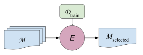
Figure 2: The typical workflow for model selection. The estimation method E tests different algorithms $\text{A}\in\mathcal{A}$ using the training data. The algorithm with best estimations is selected for predicting future observations.

The goal is to find and select $\text{A}_{*}\in\mathcal{A}$, which is the model with the best performance on the test set. The model selection problem can then be formalized as follows:

$$\text{A}_{\text{selected}}\in\underset{\text{A}\in\mathcal{A}}{\text{argmin}}\big{(}L(\text{A},\mathcal{D}_{train},E)\big{)}$$ (1)

where L represents the loss metric that quantifies the expected error of a predictive models, and E is the estimation method applied to estimate such measure.

In Equation 1, the function $L$ takes as input the learning algorithm, the training data, and the estimation method. The output of $L$ is the expected error of the respective learning algorithm. Then, the model $\text{A}_{\text{selected}}$ is selected, which is the one that minimizes the expected error. Ideally, $\text{A}_{\text{selected}}$ represents $\text{A}_{*}$, which denotes the model with best performance in a test set. However, this is not necessarily the case as $E$ is only able to provide an approximation of the true error of any model. Our goal in this paper is to analyse a set of estimation methods $\mathcal{E}=\{E_{1},E_{2},\dots,E_{q}\}$ according to their ability to find $\text{A}_{*}$, and their behavior when they do not (specifically, assess how much performance is lost). This can be regarded as an analysis of the ranking ability of the estimators, $\mathcal{E}$, in which we are particularly interested in the top ranked model. In Section 4 we present a set of experiments that compare a set of estimators from this perspective.

3.3 Average Rank

The average rank is a procedure which is typically applied to carry out a statistical comparison of multiple learning algorithms over multiple data sets brazdil2000comparison . The rank of a predictive model denotes its position in terms of performance relative to its competitors. A rank of 1 in a given data set means that the respective model was the best performing one. Effectively, the average rank represents the average relative position of a given predictive model. As Benavoli et al. benavoli2016should explain, the average rank is a non-parametric approach which does not assume normality of the sample means and is robust to outliers. This approach is often used for algorithm selection abdulrahman2018speeding .

In this work, we hypothesize that the average rank may be a useful approach for model selection within a single data set. Following Equation 1, the selected model is typically the one which minimizes the expected error. This expected error is estimated by averaging (with the arithmetic mean) the error of each model across a number of folds. However, the average error is amenable to outliers. For example, a model may incur into a large error in a single fold which will significantly effect its average. On the other hand, the average rank approach may amplify small errors brazdil2000comparison . In this context, we test whether the average rank is a better approach to combine the results of multiple models across multiple folds within the same problem.

Yang yang2007consistency explored this idea before in the context of regression tasks. The author refers to this process as voting cross-validation, and concluded that it leads to a comparable performance relative to the standard error-based cross-validation. In this work, we attempt to make this comparison for time series forecasting problems.

4 Experiments

The experiments carried out in this paper aim at comparing different estimators for model selection in time series forecasting tasks. They are designed to address the following research questions:

1. RQ1: What is the accuracy of different performance estimation methods for model selection? That is, how often do their estimates lead to picking the best model (the one which maximizes the true predictive performance in new observations);

2. RQ2: What is the forecasting performance lost when performance estimation methods do not pick the best model?

3. RQ3: Do the experimental results vary when controlling for the sample size of time series?

4. RQ4: How does the average rank (voting cross-validation) compare with the average error for aggregating the results across folds for model selection?

5. RQ5: What is the relative execution time of each estimator?

4.1 Data Sets

The experiments in this paper are carried out using 3111 real-world time series. We retrieved all the daily time series with at least 500 observations from the M4 case study makridakis2020m4 . Our query included the sample size condition (at least 500 data points) as it is an important component for the training of machine learning models cerqueira2019machine . This query returned 2937 time series. These time series are from several domains of application, including demographics, finance, industry, macro-economics, and micro-economics. The remaining 174 time series were retrieved from a previous related study cerqueira2020evaluating . 149 out of these 174 time series were retrieved from the benchmark database tsdl tsdlpackage . We also included 25 time series used by Cerqueira et al. cerqueira2019arbitrage .

4.2 Experimental Design

We create a realistic scenario to compare the different performance estimation methods for model selection. We start by splitting the available time series into two parts: an estimation set, which contains the initial 70% of observations; and a test set, which contains the subsequent 30% observations. The general goal is to select the model which provides the best performance on the test set. In practice, we cannot perform direct estimations on this set as it represents future observations. Therefore, we resort to the estimation set, which represents the available data, to estimate which is the best model.

For each estimator $E_{i}\in\mathcal{E}$, we carry out the model selection process illustrated in Figure 2 and defined in Equation 1, in which the training data represents the estimation set.

This process results in a set of models $\{\text{A}_{E_{1}},\dots,\text{A}_{E_{q}}\}$, where $A_{E_{i}}$ is the model selected by estimator $E_{i}$. Finally, we evaluate each estimator according to its model selection ability using the test set. The evaluation process is described in the next section.

4.3 Evaluation

Let $\text{A}_{E}$ denote the model selected by the estimation method E, and $\text{RMSE}(\text{A}_{E})$ its generalization root mean squared error in a given time series problem. Hopefully, $\text{A}_{E}$ is equal to $\text{A}_{*}$, which represents the best model that should be selected. In such case, $\text{RMSE}(\text{A}_{E})$ would be optimal according to the pool of available models.

We use $\text{RMSE}(\text{A}_{E})$ to quantify and compare different estimation methods. We compute the percentage difference between the error of the model selected by the estimator E ($\text{RMSE}(\text{A}_{E})$) and the error of $\text{A}_{*}$. This can be formalized as follows:

$$\text{LOSS}(E)=\frac{\text{RMSE}(\text{A}_{E})-\text{RMSE}(\text{A}_{*})}{\text{RMSE}(\text{A}_{*})}\times 100$$ (2)

where $\text{LOSS}(E)$ denotes the generalization error associated with the estimator $E$ for a given data set. This error is zero in the case E selects $\text{A}_{*}$, which is the correct choice. Otherwise, there is a positive performance loss associated with the model selection process, which is quantified by Equation 2.

If we carry this analysis with multiple time series problems, from the definition in Equation 2 we can compute the following statistics to summarise the quality of a performance estimation method for the task of model selection:

• Accuracy: how often a performance estimation method picks the best possible forecasting model. This can be quantified as the proportion of times that $\text{RMSE}(E)$ is equal to zero;

• Average Loss (AL): The average loss incurred by picking the wrong forecasting model (not selecting $\text{A}_{*}$). This loss is quantified by taking the average of each $\text{RMSE}(E)$ across all the problems when $\text{A}_{E}$ is different than $\text{A}_{*}$;

• Overall Average Loss (OAL): A combination of the two previous measurements: we compute AL but also taking into account when E selects $\text{A}_{*}$, in which case the loss is zero.

The three metrics listed above allow us to compare different estimators according to their ability to select the best forecasting model among a set of alternatives.

4.4 Learning Algorithms and Estimation Methods

For each time series problem, each estimator compares 50 alternative models, and selects the one which maximizes the expected performance. The models are obtained using different parameter settings of the following learning algorithms: support vector regression karatzoglou2004kernlab , multivariate adaptive regression splines earth , random forests ranger2015 , projection pursuit regression friedman1981projection , rule-based regression based on Cubist Cubist2014 , multi-layer perceptron monmlp2017 , generalized linear regression glmnet2010 , Gaussian processes karatzoglou2004kernlab , principal components regression plspackage , partial least squares regression plspackage , and extreme gradient boosting chen2016xgboost . The algorithms and respective parameters are described in Table 1.

Table 1: Summary of the learning algorithms

ID	Algorithm	Parameter	Value
SVR	Support Vector Regr.	Kernel	{Linear, RBF
			Polynomial, Laplace}
		Cost	{1, 5}
		$\epsilon$	{0.1, 0.01}
MARS	Multivar. A. R. Splines	Degree	{1, 3}
		No. terms	{5, 10, 20}
		Forward thresh.	{0.001}
RF	Random forest	No. trees	{250, 500}
		Mtry	{5, 10}
PPR	Proj. pursuit regr.	No. terms	{2, 4}
		Method	{super smoother, spline}
RBR	Rule-based regr.	No. iterations	{1, 5, 10, 25}
MLP	Multi-layer Perceptron	Units Hid. Lay. 1	{10, 15}
		Units Hid. Lay. 2	{0, 5}
GLM	Generalised Linear Regr.	Penalty mixing	{0, 0.25, 0.5, 0.75, 1}
GP	Gaussian Processes	Kernel	{Linear, RBF,
			Polynomial, Laplace}
		Tolerance	{0.001}
PCR	Principal Comp. Regr.	Default	-
PLS	Partial Least Regr.	Method	{kernel, SIMPLS}
XGB	Gradient Boosting	Auto	-

We focus on regression learning algorithms, which have been shown competitive forecasting performance relative to traditional approaches such as ARIMA chatfield2000time or exponential smoothing gardner1985exponential (c.f. Section 2.2).

In the experiments we apply a total of 10 performance estimation methods, which are described below:

• K-fold cross-validation (CV): First, the time series observations are randomly shuffled and split into K folds. Then, each fold is iteratively selected for testing. A model is trained on K-1 folds, and tested in the remaining one. This approach breaks the temporal order of observations, which is problematic for dependent data such as time series arlot2010survey . However, it has been shown that CV is applicable in some time series scenarios bergmeir2018note ;

• Blocked K-fold cross-validation (CV-Bl): This approach is identical to CV. The difference is that CV-Bl does not shuffle the observations before assigning them to different folds. This leads to K folds of contiguous observations. Bergmeir et al bergmeir2012use and Cerqueira et al cerqueira2020evaluating recommend this approach for estimating the performance of forecasting models if the time series is stationary;

• Modified Cross-validation (CV-Mod): The modified cross-validation is a variant of CV which attempts at decreasing the dependency between training and testing observations mcquarrie1998regression . First, time series observations are randomly shuffled into K folds, similarly to CV. Then, in each iteration of the cross-validation procedure, some of the training observations are removed. Particularly, we remove the training observations which are within $p$ (the size of the auto-regressive process) observations of any testing point. While this process increases the independence among observations, a considerable number of observations are removed;

• hv-Blocked K-fold cross-validation (CV-hvBl): The hv-blocked K-fold cross-validation racine2000consistent is a variant of CV-Bl. Similarly to CV-Mod, it removes some instances to decrease the dependency among observations. Specifically, for each iteration, the adjacent $p$ observations between training and testing are removed. This process creates a small gap between the two sets;

• Holdout: This method represents the typical out-of-sample estimation approach, in which the final part of the time series is held out for testing. This process runs in a single iteration, in which the initial 70% of observations are used for training, while the subsequent 30% ones used for testing;

• Repeated Holdout (Rep-Holdout): An extension of Holdout in which this process is repeated K times in multiple, randomized, testing periods tashman2000out ; cerqueira2020evaluating . For each one of the K iterations, a random point is chosen in the time series. Then, the 60% observations (out of the total time series length n) before this point are used for training, while the subsequent 10% observations (out of n) are used for testing. Note that the window for selecting this random point is restricted by the size of the training and testing sets cerqueira2020evaluating ;

• Prequential in Blocks (Preq-Bls): We apply the prequential evaluation methodology using K blocks of data and a growing window dawid1984present . In the first iteration, the initial block containing the first n/K observations is used for training, while the subsequent block (also containing n/K observations) is used for testing. Afterwards, these two blocks are merged together, and used for training in the second iteration. In this iteration, the third block of data is used for testing. This process continues until the last block is tested. The Preq-Bls procedure is commonly used for evaluating time series models. This method is often referred to as time series cross-validation^,;

• Prequential in Sliding Blocks (Preq-Sld-Bls): This method represents a variant of Preq-Bls but applied with a sliding window. This means that, after each iteration, the oldest block of data is discarded. Therefore, in each iteration a single block of observations is used for training, and another one is used for testing;

• Trimmed Prequential in Blocks (Preq-Bls-Trim): A variant of Preq-Bls in which the initial splits are discarded due to low sample size: The initial iterations use a training sample size that may not be representative of the complete available time series, which may bias the results. Formally, according to this method, only the final 60% of the K iterations of the Preq-Bls procedure are considered. For example, if Preq-Bls splits the time series into 10 blocks, the method Preq-Bls-Trim only considers (and averages) the results on the last 60% (i.e. 6) iterations;

• Prequential in Blocks with a Gap (Preq-Bls-Gap): A final variant of Preq-Bls, in which a gap is introduced between the training and testing sets. In each iteration, there is a block of n/K observations splitting the training and test sets. Similarly to CV-Mod e CV-hvBl, the motivation for this process is to increase the independence between the two sets.

We refer to the work by Cerqueira et al. cerqueira2020evaluating for more information on these methods, including visual representations. We use two approaches to combine the results of the K iterations of each estimator: the average error according to the arithmetic mean, and the average rank.

4.5 Parameter Settings

The number of lags p (c.f. Section 3.1) used in each time series is set according to the False Nearest Neighbors method kennel1992determining , which is a common approach in non-linear time series analysis. The number of folds or repetitions K of the estimation methods is set to 10, where applicable.

4.6 Results

We present the main results in Table 2, which shows the score of each estimator over the 3111 time series, both for the average error and average rank approaches. In the table, the methods are ordered by increasing values of OAL, obtained either by average rank or average error.

4.6.1 RQ1: Accuracy of the Estimators

Table 2: Results for all method over the 3111 time series. Methods are ordered by increasing values of overall average loss. Each metrics is bold according to which approach (average rank or average error) provides the best result for each estimator.

	Average Error			Average Rank
	Acc.	AL	OAL	Acc.	AL	OAL
CV-Bl	0.10	0.34$\pm$0.72	0.29$\pm$0.68	0.08	0.32$\pm$0.64	0.28$\pm$0.64
Preq-Bls	0.09	0.33$\pm$0.70	0.28$\pm$0.68	0.08	0.34$\pm$0.68	0.30$\pm$0.66
CV-hvBl	0.10	0.35$\pm$0.72	0.30$\pm$0.69	0.09	0.33$\pm$0.64	0.28$\pm$0.63
CV-Mod	0.07	0.33$\pm$0.68	0.30$\pm$0.66	0.06	0.35$\pm$0.70	0.31$\pm$0.68
Preq-Bls-Gap	0.09	0.36$\pm$0.79	0.30$\pm$0.75	0.07	0.37$\pm$0.73	0.32$\pm$0.70
CV	0.09	0.38$\pm$0.82	0.32$\pm$0.78	0.07	0.40$\pm$0.74	0.35$\pm$0.73
Preq-Sld-Bls	0.07	0.39$\pm$1.06	0.34$\pm$1.03	0.06	0.37$\pm$0.99	0.33$\pm$0.93
Preq-Bls-Trim	0.09	0.41$\pm$0.86	0.35$\pm$0.83	0.08	0.40$\pm$0.76	0.35$\pm$0.74
Rep-Holdout	0.08	0.42$\pm$0.88	0.35$\pm$0.85	0.07	0.40$\pm$0.79	0.36$\pm$0.75
Holdout	0.07	0.67$\pm$1.79	0.58$\pm$1.64	0.07	0.67$\pm$1.79	0.58$\pm$1.64

The accuracy of the estimators for finding the best predictive model ranges from 7% to 10%. These values represent a significant improvement relatively to a random selection procedure, which has an expected accuracy of 2% (1 over 50 possible alternative models). Notwithstanding, this degree of accuracy across all methods means that a given estimator will most probably fail to select the most appropriate model in the available pool. In relative terms, CV-Bl and CV-hvBl show the best score (10%) while CV-Mod, Preq-Sld-Bls, and Holdout show the worst one (7%).

Overall, the accuracy scores for finding the best predictive model highlights the importance of studying the subsequent shortfall: how much forecasting performance is lost by picking the wrong model.

4.6.2 RQ2: Performance Loss During Model Selection

The AL and OAL scores quantify the average performance loss of the estimator. We present both for completeness but will focus on the OAL metric in our analysis because it also incorporates the cases in which the estimator selects the correct model.

The scores of OAL range from 0.28% (CV-Bl, Preq-Bls, and CV-hvBl) and 0.58% (Holdout). As explained before, this metric represents the average (median) difference between the loss of the forecasting model selected by the respective estimator and the loss of the best possible solution available, in which the average is computed across all time series. Essentially, if we apply one of the best estimators we can expect a performance loss of about 0.28% with respect to the best predictive model in the available pool. Note that these results are highly dependent on the particular pool of available forecasting algorithms. The values for average loss are significant. In many domains of application, each increment in forecasting performance has a considerable financial impact within organizations jain2017answers . Therefore, it is crucial to maximize this performance. However, unless the domain is sensitive to small differences in performance, the chosen estimation method is not a critical factor for performance.

Overall, except for Holdout which shows an OAL significantly higher than the rest, the results are comparable across all estimation methods. Especially when considering the dispersion (IQR), which is quite significant. Even the standard cross-validation procedure (CV), which is a poor method for performance estimation for forecasting cerqueira2020evaluating , only shows a OAL difference of 0.04% to the best estimators. This shows that breaking the temporal order of observations during model selection is, in general, not problematic for time series forecasting tasks.

In general, all estimators present a considerable variability in both AL and OAL. We explore the dispersion further in Figure 3, which shows the distribution of the loss of each estimator relative to the oracle. This loss is non-negative and, as described before, it is zero when the estimator selects the best possible solution. The figure shows that all estimators incur in large errors in some data sets. This means that, while the median errors are comparable, one may be exposed to a significant performance loss irrespective of the estimation method used.

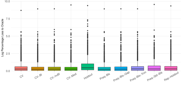
Figure 3: Distribution of the OAL (log-scaled) incurred by each estimation method with respect to the Oracle using all time series. The results suggest a large number of outliers for all methods.

4.6.3 RQ3: Sensitivity Analysis on the Sample Size

In this section, we analyse the effect of the time series sample size in the experimental results. A previous study by Cerqueira et al. cerqueira2019machine showed that the training sample size of time series is an important factor in the relative forecasting performance among different predictive models. We aim at studying this effect in estimation methods when applied for model selection. To accomplish this, we split the time series into two groups: a group which consists of 371 time series (out of 3111) with less than 1000 observations; and another group with 2740 time series with sample size above 1000 data points. Then, we carry out the previous analysis for each group of time series.

Table 3: Results for each method in 371 time series with sample size below 1000 observations. Methods are ordered by increasing values of overall average loss. Each metrics is bold according to which approach (average rank or average error) provides the best result for each estimator.

	Average Error			Average Rank
	Acc.	AL	OAL	Acc.	AL	OAL
CV-hvBl	0.09	1.53$\pm$2.96	1.28$\pm$2.89	0.06	1.35$\pm$2.67	1.19$\pm$2.41
CV	0.08	1.45$\pm$3.08	1.30$\pm$2.78	0.09	1.45$\pm$3.10	1.21$\pm$2.79
Preq-Bls-Trim	0.08	1.66$\pm$3.29	1.39$\pm$3.19	0.07	1.46$\pm$2.91	1.30$\pm$2.76
CV-Mod	0.07	1.54$\pm$2.93	1.33$\pm$2.95	0.05	1.54$\pm$3.14	1.34$\pm$3.04
CV-Bl	0.08	1.55$\pm$2.97	1.34$\pm$2.88	0.06	1.53$\pm$2.83	1.38$\pm$2.70
Rep-Holdout	0.09	1.64$\pm$3.22	1.40$\pm$2.96	0.07	1.57$\pm$2.80	1.36$\pm$2.74
Preq-Bls-Gap	0.07	1.65$\pm$3.21	1.48$\pm$3.01	0.06	1.53$\pm$3.21	1.36$\pm$3.05
Preq-Bls	0.08	1.60$\pm$2.72	1.39$\pm$2.65	0.06	1.59$\pm$3.13	1.44$\pm$2.89
Preq-Sld-Bls	0.04	1.77$\pm$3.23	1.70$\pm$3.19	0.02	1.79$\pm$2.97	1.76$\pm$2.98
Holdout	0.06	2.43$\pm$5.75	2.25$\pm$5.77	0.06	2.43$\pm$5.75	2.25$\pm$5.77

Table 4: Results for each method in 2740 time series with sample size above 1000 observations. Methods are ordered by increasing values of overall average loss. Each metrics is bold according to which approach (average rank or average error) provides the best result for each estimator.

	Average Error			Average Rank
	Acc.	AL	OAL	Acc.	AL	OAL
Preq-Bls	0.09	0.29$\pm$0.58	0.24$\pm$0.57	0.08	0.30$\pm$0.56	0.26$\pm$0.56
CV-Bl	0.10	0.30$\pm$0.56	0.25$\pm$0.56	0.09	0.28$\pm$0.52	0.24$\pm$0.52
CV-hvBl	0.10	0.30$\pm$0.57	0.26$\pm$0.57	0.09	0.29$\pm$0.53	0.24$\pm$0.51
CV-Mod	0.07	0.30$\pm$0.54	0.26$\pm$0.53	0.06	0.30$\pm$0.56	0.28$\pm$0.56
Preq-Bls-Gap	0.09	0.31$\pm$0.60	0.26$\pm$0.61	0.07	0.32$\pm$0.57	0.28$\pm$0.58
Preq-Sld-Bls	0.07	0.33$\pm$0.81	0.28$\pm$0.77	0.07	0.31$\pm$0.73	0.27$\pm$0.69
CV	0.09	0.33$\pm$0.65	0.29$\pm$0.62	0.07	0.35$\pm$0.60	0.32$\pm$0.60
Preq-Bls-Trim	0.09	0.36$\pm$0.69	0.30$\pm$0.68	0.08	0.35$\pm$0.61	0.31$\pm$0.61
Rep-Holdout	0.08	0.36$\pm$0.70	0.30$\pm$0.68	0.07	0.35$\pm$0.63	0.31$\pm$0.62
Holdout	0.07	0.59$\pm$1.41	0.51$\pm$1.33	0.07	0.59$\pm$1.41	0.51$\pm$1.33

The results are shown in Tables 3 and 4, in which the first presents the results for the time series with low sample size, and the second shows the results for the group of time series with sample size above 1000 observations. There are considerable differences across the two groups. All metrics are noticeably better for larger sample sizes. This result indicates that the model selection task is easier for all estimators if more data is available, which is not surprising.

The results for the group of larger time series (more than 1000 observations) do not vary considerably with respect to the results show in Table 2 for all time series. This is expected because most of the available time series are part of this group. Notwithstanding, the group of smaller time series (less than 1000 data points) contains 371 time series, which is a considerable amount. In terms of relative performance for this group of time series, CV-hvBl, CV, and Preq-Bls-Trim show the best estimation ability.

An interesting result is how much Preq-Bls-Trim improved relative to Preq-Bls in the group of small time series. As a reminder, Preq-Bls is a common procedure used to evaluate predictive models applied in time-dependent scenarios. For example, this strategy is implemented in the widely used scikit-learn pedregosa2011scikit Python library as TimeSeriesSplits. Our results show that Preq-Bls-Trim, which discards the initial iterations of Preq-Bls, presents better results for smaller time series while requiring less computational resources. A possible explanation is the following. Since the sample size is low, the initial iterations of the estimation procedure may not be representative of the complete time series, and leads to a poor model selection by Preq-Bls. By discarding the initial iterations we keep only those folds which are more representative of the complete time series.

4.6.4 RQ4: Analysis of the Averaging Approaches

Regarding the comparison between average error and average rank (also known as voting cross-validation yang2007consistency ), the results are comparable. The average error leads to a systematic, but marginal, better accuracy. Across all data sets, the AL and OAL scores are comparable. The average rank shows a slightly better AL and OAL scores when the time series comprises less than 1000 observations. Note that, in the case of Holdout, the average error and average rank are identical because this estimator relies on a single iteration. Since the average rank requires the extra computation of computing ranks, the average error may be a preferable approach for simplicity.

4.6.5 RQ5: Execution Time Analysis

Finally, we analyse the execution time of each estimator. The execution time denotes the time a given estimator takes to carry out the estimation process and produce a ranking of the predictive models under comparison.

The results of this analysis are shown in Figure 4, which shows the distribution of the execution time of each estimator across the 3111 data sets. The estimators are ordered (from left to right) by median execution time. Holdout is the quickest estimator while CV is the slowest one, on average. In general, the execution time is correlated with the number of iterations and amount of data used by the estimator.

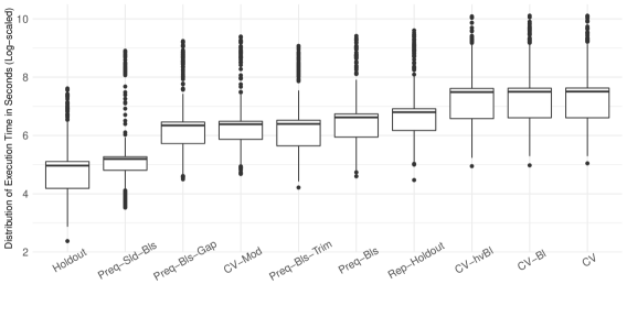
Figure 4: Distribution of the execution time in seconds (log-scaled), of each estimator across the 3111 time series.

5 Discussion

We analysed the ability of several estimators for model selection in time series forecasting tasks. We carried out experiments using 3111 univariate time series, 10 estimation methods, and 50 auto-regressive models. We emulated a realistic scenario in which each estimator tests each one of the 50 models using the available data, and selects one for making predictions in a test set.

We discovered that, given the number of possible alternative models (50), all estimators show a low accuracy for selecting the best available model (RQ1) (though the scores are significantly better relative to a random selection procedure). Accordingly, this lead us to study the difference in performance between the model selected by each estimator and the model that should have been selected (the one maximizing forecasting performance on test data). Overall, the average difference across all time series ranges from about 0.28% to about 0.58%. However, there is a large variability in the results across all estimation methods (RQ2). These values may be significant in many domains, and show that the evaluation process of time series models is an important task that should not be overlooked.

We found that the results vary considerably when controlling for time series sample size. For larger time series (comprising more than 1000 observations), the results are consistent to the conclusions presented above. On the other hand, the model selection task is significantly more difficult when smaller sample sizes are available for all estimation methods. The best overall estimator incurs into an average performance loss of 0.28%, but this value increases to 1.19% for the group of time series with less than 1000 data points (RQ3).

Finally, we analysed the execution time of each approach. We found that the values are correlated with the amount of data each estimator use (RQ4).

We found considerable distinctions in the relative performance of the estimators when applied for performance estimation cerqueira2020evaluating and when used for model selection. For performance estimation, Cerqueira et al. cerqueira2020evaluating report that CV is the worst estimator, across the 174 time series that they study. For model selection purposes, which is the topic of the current paper, CV is actually competitive with the best approaches, especially for smaller sample sizes. Cerqueira et al. cerqueira2020evaluating did not find any impact by the time series sample size in the relative performance of the estimators. We found this factor to be important for model selection, though it is important to remark that the process for analysing this impact is different in the two studies. Moreover, this impact is noticeable both in relative terms, where the ranking of the estimators is different, and in absolute terms, in the sense that larger sample sizes lead to a better overall model selection results.

In terms of OAL there is a 0.3% gap between the best estimator (CV-Bl applied with average rank) and the worst estimator (Holdout). This gap decreases to 0.06% if we ignore Holdout, which performs systematically worse than the other approaches. The significance of the differences in the OAL scores diminishes further when inspecting the dispersion (using IQR) across the time series, which is often more than double the average score. In this context, we conclude that there is no significant difference between the estimators analysed in this work. The exception is Holdout, which we believe should be avoided unless a large sample size is available.

6 Conclusions

We study different estimation methods for performing model selection in time series forecasting tasks. While these methods have been studied for performance estimation bergmeir2012use ; bergmeir2018note ; cerqueira2020evaluating , model selection is a different problem. Therefore, the best estimator for performing model selection may not be the most appropriate for performance estimation.

Our goal in this paper was to analyse the accuracy of each estimator for selecting the most appropriate model, and the respective forecasting performance loss when they do not. We carried out a set of experiments using 3111 time series, 10 estimation methods, and 50 predictive models to achieve this goal.

We found that the overall performance loss during model selection revolves between 0.28% and 0.58%. We also discovered that taking the average rank of models, instead of the average error, leads to a comparable performance in terms of model selection. In terms of relative performance, we conclude that all estimation methods behave comparably for model selection as their performance differences are negligible. This means that while previous studies have show significant differences between these methods for estimating the performance of the models, when our goal is to select among them, these differences disappear. The exception is Holdout, which should be avoided unless there is a large sample size available. The experiments carried out in the paper are available in an online repository.

References

- (1) Abdulrahman, S.M., Brazdil, P., van Rijn, J.N., Vanschoren, J.: Speeding up algorithm selection using average ranking and active testing by introducing runtime. Machine learning 107(1), 79–108 (2018)
- (2) Arlot, S., Celisse, A., et al.: A survey of cross-validation procedures for model selection. Statistics surveys 4, 40–79 (2010)
- (3) Benavoli, A., Corani, G., Mangili, F.: Should we really use post-hoc tests based on mean-ranks? The Journal of Machine Learning Research 17(1), 152–161 (2016)
- (4) Bergmeir, C., Benítez, J.M.: On the use of cross-validation for time series predictor evaluation. Information Sciences 191, 192–213 (2012)
- (5) Bergmeir, C., Hyndman, R.J., Koo, B.: A note on the validity of cross-validation for evaluating autoregressive time series prediction. Computational Statistics & Data Analysis 120, 70–83 (2018)
- (6) Brazdil, P.B., Soares, C.: A comparison of ranking methods for classification algorithm selection. In: European conference on machine learning, pp. 63–75. Springer (2000)
- (7) Breiman, L., Spector, P.: Submodel selection and evaluation in regression. the x-random case. International statistical review/revue internationale de Statistique pp. 291–319 (1992)
- (8) Cannon, A.J.: monmlp: Multi-Layer Perceptron Neural Network with Optional Monotonicity Constraints (2017). URL https://CRAN.R-project.org/package=monmlp. R package version 1.1.5
- (9) Cerqueira, V., Torgo, L., Mozetič, I.: Evaluating time series forecasting models: An empirical study on performance estimation methods. Machine Learning pp. 1–32 (2020)
- (10) Cerqueira, V., Torgo, L., Oliveira, M., Pfahringer, B.: Dynamic and heterogeneous ensembles for time series forecasting. In: 2017 IEEE International Conference on Data Science and Advanced Analytics (DSAA), pp. 242–251. IEEE (2017)
- (11) Cerqueira, V., Torgo, L., Pinto, F., Soares, C.: Arbitrage of forecasting experts. Machine Learning 108(6), 913–944 (2019)
- (12) Cerqueira, V., Torgo, L., Soares, C.: Machine learning vs statistical methods for time series forecasting: Size matters. arXiv preprint arXiv:1909.13316 (2019)
- (13) Chatfield, C.: Time-series forecasting. CRC press (2000)
- (14) Chen, T., Guestrin, C.: Xgboost: A scalable tree boosting system. In: Proceedings of the 22nd acm sigkdd international conference on knowledge discovery and data mining, pp. 785–794 (2016)
- (15) Corani, G., Benavoli, A., Augusto, J., Zaffalon, M.: Automatic forecasting using gaussian processes. arXiv preprint arXiv:2009.08102 (2020)
- (16) Dawid, A.P.: Present position and potential developments: Some personal views statistical theory the prequential approach. Journal of the Royal Statistical Society: Series A (General) 147(2), 278–290 (1984)
- (17) Friedman, J., Hastie, T., Tibshirani, R.: Regularization paths for generalized linear models via coordinate descent. Journal of Statistical Software 33(1), 1–22 (2010)
- (18) Friedman, J.H., Stuetzle, W.: Projection pursuit regression. Journal of the American statistical Association 76(376), 817–823 (1981)
- (19) Gama, J., Rodrigues, P.P., Sebastião, R.: Evaluating algorithms that learn from data streams. In: Proceedings of the 2009 ACM symposium on Applied Computing, pp. 1496–1500 (2009)
- (20) Gardner Jr, E.S.: Exponential smoothing: The state of the art. Journal of forecasting 4(1), 1–28 (1985)
- (21) Hyndman, R., Yang, Y.: tsdl: Time Series Data Library (2019). Https://finyang.github.io/tsdl/, https://github.com/FinYang/tsdl
- (22) Jain, C.L.: Answers to your forecasting questions. The Journal of Business Forecasting 36(1), 3 (2017)
- (23) Karatzoglou, A., Smola, A., Hornik, K., Zeileis, A.: kernlab-an s4 package for kernel methods in r. Journal of statistical software 11(9), 1–20 (2004)
- (24) Ke, G., Meng, Q., Finley, T., Wang, T., Chen, W., Ma, W., Ye, Q., Liu, T.Y.: Lightgbm: A highly efficient gradient boosting decision tree. In: Advances in neural information processing systems, pp. 3146–3154 (2017)
- (25) Kennel, M.B., Brown, R., Abarbanel, H.D.: Determining embedding dimension for phase-space reconstruction using a geometrical construction. Physical review A 45(6), 3403 (1992)
- (26) Kuhn, M., Weston, S., Keefer, C., code for Cubist by Ross Quinlan, N.C.C.: Cubist: Rule- and Instance-Based Regression Modeling (2014). R package version 0.0.18
- (27) Makridakis, S., Spiliotis, E., Assimakopoulos, V.: Statistical and machine learning forecasting methods: Concerns and ways forward. PloS one 13(3), e0194,889 (2018)
- (28) Makridakis, S., Spiliotis, E., Assimakopoulos, V.: The m4 competition: 100,000 time series and 61 forecasting methods. International Journal of Forecasting 36(1), 54–74 (2020)
- (29) Makridakis, S., Spiliotis, E., Assimakopoulos, V.: The m5 accuracy competition: Results, findings and conclusions. Int J Forecast (2020)
- (30) McQuarrie, A.D., Tsai, C.L.: Regression and time series model selection. World Scientific (1998)
- (31) Mevik, B.H., Wehrens, R., Liland, K.H.: pls: Partial Least Squares and Principal Component Regression (2016). URL https://CRAN.R-project.org/package=pls. R package version 2.6-0
- (32) Milborrow, S.: earth: Multivariate Adaptive Regression Spline Models (2012)
- (33) Mozetič, I., Torgo, L., Cerqueira, V., Smailović, J.: How to evaluate sentiment classifiers for twitter time-ordered data? PloS one 13(3), e0194,317 (2018)
- (34) Opsomer, J., Wang, Y., Yang, Y.: Nonparametric regression with correlated errors. Statistical Science pp. 134–153 (2001)
- (35) Oreshkin, B.N., Carpov, D., Chapados, N., Bengio, Y.: N-beats: Neural basis expansion analysis for interpretable time series forecasting. arXiv preprint arXiv:1905.10437 (2019)
- (36) Pedregosa, F., Varoquaux, G., Gramfort, A., Michel, V., Thirion, B., Grisel, O., Blondel, M., Prettenhofer, P., Weiss, R., Dubourg, V., et al.: Scikit-learn: Machine learning in python. the Journal of machine Learning research 12, 2825–2830 (2011)
- (37) Racine, J.: Consistent cross-validatory model-selection for dependent data: hv-block cross-validation. Journal of econometrics 99(1), 39–61 (2000)
- (38) Salinas, D., Flunkert, V., Gasthaus, J., Januschowski, T.: Deepar: Probabilistic forecasting with autoregressive recurrent networks. International Journal of Forecasting 36(3), 1181–1191 (2020)
- (39) Smyl, S.: A hybrid method of exponential smoothing and recurrent neural networks for time series forecasting. International Journal of Forecasting 36(1), 75–85 (2020)
- (40) Snijders, T.A.: On cross-validation for predictor evaluation in time series. In: On model uncertainty and its statistical implications, pp. 56–69. Springer (1988)
- (41) Spiliotis, E., Makridakis, S., Semenoglou, A.A., Assimakopoulos, V.: Comparison of statistical and machine learning methods for daily sku demand forecasting. Operational Research pp. 1–25 (2020)
- (42) Tashman, L.J.: Out-of-sample tests of forecasting accuracy: an analysis and review. International journal of forecasting 16(4), 437–450 (2000)
- (43) Wright, M.N.: ranger: A Fast Implementation of Random Forests (2015). R package
- (44) Yang, Y.: Consistency of cross validation for comparing regression procedures. The Annals of Statistics 35(6), 2450–2473 (2007)