Is the remnant of GW190425 a strange quark star?

Abstract

This study investigates the effects of different QCD models on the structure of strange quark stars (SQS). In these models, the running coupling constant has a finite value in the infrared region of energy. By imposing some constraints on the strange quark matter (SQM) and exploiting the analytic and background perturbation theories, the equations of states for the SQM are obtained. Then, the properties of SQSs in general relativity are evaluated. By using component masses of GW190425 Abbott2020ApJL as well as some conversion relations between the baryonic mass and the gravitational mass, the remnant mass of GW190425 is obtained. Our results for the maximum gravitational mass of SQS are then compared with the remnant mass of GW190425. The results indicate that the obtained maximum gravitational masses are comparable to the remnant mass of GW190425. Therefore, it is proposed that the remnant mass of GW190425 might be a SQS.

I Introduction

Compact stars are considered large laboratories for investigating quantum chromodynamics (QCD) models. One of the most challenging issues in QCD is the running coupling constant’s infrared (IR) scale behavior. The running coupling constant obtained from the renormalization procedure and the renormalization group equations has a well-defined behavior at large momenta Prosperi2007 ; Altarelli2013 . However, it becomes infinite at a point in the IR scale called the Landau pole ($\Lambda$). Based on the perturbative QCD, the quark confinement originates from the Landau pole, which depends on the selected renormalization scheme Deur2016 . Nevertheless, the data extracted from some experiments indicate that the running coupling constant of QCD at low momenta is finite and freezes to a constant value Deur2016 . For example, the effective strong coupling constant ($\alpha_{s,g1}(Q^{2})$) defined based on the Bjorken sum rule has been extracted from the CLAS spectrometer Deur2008 where the polarized electron beam (with energies ranging from $1$ to $6$$GeV$) collides with proton and deuteron targets. The data show that $\alpha_{s,g1}(Q^{2})$ loses its scale dependence at low momenta. In Ref. Perez-Ramos2010 , by analyzing the energy spectra of heavy quark jets from $e^{+}e^{-}$ annihilation, the IR value for the effective coupling constant ($\alpha_{s}^{eff}(Q)$), is obtained as $\left(2GeV\right)^{-1}\int_{0}^{2GeV}(\alpha_{s}^{eff}(Q)/{\pi})dQ=0.18\pm 0.01$. Using the data of hadronic decays of the $\tau$-lepton extracted from the OPAL detector at LEP OPAL1999 , it is shown that for a hypothetical $\tau$-lepton with the mass of $m_{\tau^{{}^{\prime}}}$, the effective charge $\alpha_{\tau}(m_{\tau^{{}^{\prime}}}^{2})$, freezes at the mass scale of $m_{\tau^{{}^{\prime}}}^{2}\cong 1GeV^{2}$ with the magnitude of $0.9\pm 0.1$ Brodsky2003 . Such behavior of the coupling constant at low momenta is called IR freezing in the literature. This effect can be explained by the running behavior of the coupling constant, which stems from particle-antiparticle loop corrections. Due to confinement, quarks and antiquarks cannot have a wavelength larger than the size of the hadron. This suppresses the loop corrections at the IR scale. Consequently, $\alpha_{s}$ is expected to lose its energy dependence at low energies Brodsky2008 . In addition, the theoretical results from the Lattice QCD Bali2001 and the Schwinger-Dyson framework Fischer2006 , show that $\alpha_{s}$ freezes at low momenta. There are other models, such as the Stochastic quantization approach Zwanziger2002 , the optimized perturbation theory Mattingly1992 , the Gribov-Zwanziger approach Gracey2006 , and the background perturbation theory Badalian1997 ; Simonov2011 , in all of which $\alpha_{s}$ runs with an IR freezing effect. Moreover, the analytic perturbation theory presents a running coupling constant with a slowly varying behavior at low energies Shirkov1997 . It should be noted that for the quark confinement, the coupling constant does not need to be infinite in the IR region. For example, the lattice simulations show that the $q\bar{q}$ potential increases linearly at distances larger than $0.4fm$, while the coupling constant freezes at a maximum value Bali2006 . Contrary to general belief, the value of the coupling constant does not need to be infinite in the IR region in order to confine light quarks Gribov1999 .

This paper first investigates the IR behavior of the QCD running coupling constant in different models. Then, two models are selected for the perturbative calculation of the equations of states (EOSs) of strange quark matter (SQM) in the leading order of $\alpha_{s}$. These two models are i) the analytic perturbation theory (APT) and ii) the background perturbation theory (BPT). Afterward, the EOSs are used in the TOV equation to calculate the maximum gravitational masses of strange quark stars (SQSs). Motivated by the LIGO detection of the compact binary coalescence (GW190425) with the total mass of $3.4_{-0.1}^{+0.3}{M}_{\odot}$ Abbott2020ApJL , we compared our results with the remnant mass of GW190425. This binary is more massive than the other reported Galactic double neutron stars (NSs) Farrow2019 . Since no electromagnetic counterpart has been observed for GW190425, its origin is unknown Kyutoku2020 . Various models have suggested the nature of GW190425. In Ref. Kyutoku2020 , the possibility of whether GW190425 is a binary NS merger or a black hole-NS (BH-NS) merger has been investigated. It is hypothesized that the progenitor of GW190425 is a binary including a NS and a $4-5M_{\odot}$ helium star Romero-Shaw2020 . Furthermore, it is suggested that GW190425 is a NS-BH merger with the masses of $1.15_{-0.13}^{+0.15}{M}_{\odot}$ and $2.4_{-0.32}^{+0.36}{M}_{\odot}$ for the NS and the BH, respectively Han2020 . In addition, using a toy model, some researchers have investigated whether future LISA observations could detect binary NSs like GW190425 Korol2021 . In Ref. Clesse2020 , GW190425 and GW190814 have been investigated as primordial BH clusters. In this paper, it is not intended to probe the nature of GW190425. Rather, the aim is to explore whether the remnant mass of GW190425 is a SQS. In this study, it is shown that the maximum gravitational masses of SQSs are comparable with the remnant mass of GW190425.

In this paper, we consider a pure SQS whose degrees of freedom are quarks (up, down, and strange flavors) and gluons. However, in a realistic description of SQS, the phase of the hadronic matter (nucleons and hyperons) could occur at low densities at the star’s surface Nandi2018 ; EslamPanah2019a ; Li2021 . An important quantity representing the SQM phase is the ratio of energy density to the baryon number density, $\epsilon/n_{B}$ at zero pressure. The value of $\epsilon/n_{B}$ should be less than that of the most stable nuclide (${}^{56}Fe$), $\epsilon/n_{B}=930MeV$. While this condition is expected to occur at densities greater than $n_{B}=0.16fm^{-3}$, we show that the above condition ($\epsilon/n_{B}<930MeV$) can occur at lower densities in the models used in this paper. This happens by employing a set of equations coming from the chemical equilibrium and the charge neutrality conditions and also imposing the following constraints for SQM. I) The ratio of $\epsilon/n_{B}$ at zero pressure should be lower than $930MeV$. II) The perturbative term has to be lower than the free term. III) The number density of strange quark must be non-zero. The onset density is obtained to be $n_{B}\sim 0.1fm^{-3}$ which shows that SQM phase can occur in $n_{B}<0.16fm^{-3}$. in Ref. Kurkela2010 , by using perturbative calculation, the same behavior is shown to be true ($n_{B}\sim 0.15fm^{-3}$). The reason for obtaining a lower density in this paper is due to the fact that we use a modified QCD running coupling constant. However, one might say that the onset density of the quark matter might be greater than the value obtained from the leading order perturbative calculations, and considering the higher-order terms in perturbation leads to higher values for onset density of SQM. For this issue, we have also used other values of onset density of SQM, including 0.128 $fm^{-3}$ and $0.155fm^{-3}$. We do not consider confining effects for the following reason. The static potential $V(r)$ is divided into two parts, including $V_{NP}(r)$ and $V_{GE}(r)$ as the non-perturbative (NP) confining potential and the gluon-exchange term, respectively. $V_{NP}(r)$ appears at $q\bar{q}$ separations for $r>T_{g}$, where $T_{g}$ is the gluonic correlation length, $T_{g}\sim 0.2fm^{-3}$ Badalian2005 . At zero temperature and finite chemical potential with $N_{f}$ flavor, the phenomenological models suggest $Q=[1\overline{\mu}-4\overline{\mu}](\overline{\mu}\equiv\sum_{f}\mu_{f}/3)$ Schneider2003 ; Karmakar2019 ; Bandyopadhyay2019 ; Kurkela2010 . We set the maximum value for $Q$ ($Q=4\overline{\mu}$) to find the maximum possible mass of the SQS in our models and minimize the confinement effects. However, we found that for $Q\gtrsim 3.4(\mu_{u}+\mu_{d}+\mu_{s})/3$, the results for the structural properties of SQS do not change considerably (see appendix C for more details). By considering $Q=4(\mu_{u}+\mu_{d}+\mu_{s})/3$, the onset densities $0.1fm^{-3}$, $0.128fm^{-3}$ and $0.155fm^{-3}$ lead to the range of $r\lesssim 0.206fm$, $r\lesssim 0.195fm$ and $r\lesssim 0.185fm$, respectively. The value of $r$ is speculated by the uncertainty relation ($r\times Q\simeq\hbar$). By solving charge neutrality and beta equilibrium equations for each onset density, we obtain the minimum chemical potential values for each quark flavor and, consequently, the minimum value of $Q$. Then by uncertainty relation, the maximum value of $r$ is obtained. It is worth mentioning that in Ref. Kurkela2010 , it is discussed that for the renormalization scales, $Q<0.8GeV$, the perturbative calculations are unreliable due to different uncertainties in the values of strange quark mass and coupling constant. Meanwhile in our calculations, the onset densities $0.1fm^{-3}$, $0.128fm^{-3}$ and $0.155fm^{-3}$ correspond to $Q>0.955GeV$, $Q>1.01GeV$ and $Q>1.06GeV$, which shows that our results are reliable.

II IR behavior of $\alpha_{s}$ in different models

As discussed above, there are experimental evidences and models which support the slowly varying or freezing behavior of the running coupling constant in the IR region. However, there is no consensus on the freezing point and the corresponding value of the coupling constant. In this section, the running coupling constant behaviors of different QCD models in the IR $Q^{2}$ are investigated. These models are as follows: i) regular perturbation theory (RPT); ii) APT; iii) BPT; iv) flux-tube model (FTM) Godfrey1985 ; and v) Cornwall Schwinger-Dyson equation (CSD) Cornwall1982 . The behavior of the running coupling constant in these models for $Q<3GeV$ is shown in Figure. 1. According to this figure, as $Q$ decreases in the IR region, $\alpha_{APT}$ varies much more slowly than $\alpha_{RPT}$. Nevertheless, compared to the other models, $\alpha_{APT}$ increases faster in the IR region, especially for $Q<0.7$$GeV$. The couplings of the BPT, FTM, and CSD models have so slowly varying behavior in the IR momenta that it can be said that they freeze compared to the couplings of RPT and APT. However, for ultraviolet (UV) momenta, all the models have an asymptotic behavior and coincide with each other. Two of the mentioned coupling constants (except for that of RPT) with higher values in the IR region are used. After a brief description of these models, they are used to calculate the perturbative EOSs of SQM. The models are as follows:

$1$) APT: The analytic coupling constant ($\alpha_{an}$) at one-loop approximation Shirkov1997 is derived in Appendix A as

$$\alpha_{APT}^{(1)}\left(Q^{2}\right)=4\pi/\beta_{0}\left[\left(\ln\left(\frac{Q^{2}}{\Lambda^{2}}\right)\right)^{-1}+\frac{\Lambda^{2}}{\Lambda^{2}-Q^{2}}\right].$$ (1)

Supposing that $N_{c}$ and $N_{f}$ are the number of colors and flavors respectively, $\beta_{0}$ is defined as $\frac{11N_{c}-2N_{f}}{3}$. It can be seen that this running coupling constant has $Q^{2}$ analyticity at all points and decreases monotonously in the IR region without any divergence Deur2016 . The interesting feature of this running coupling is that $\alpha_{an}\left(Q^{2}=0\right)=4\pi/\beta_{0}$ has no dependence on the QCD scale parameter ($\Lambda$). Furthermore, all perturbative orders of $\alpha_{an}$ have the same value at $Q^{2}=0$. Hence, it is expected that different orders of $\alpha_{an}\left(Q^{2}\right)$ have close values. For example, in the $\overline{MS}$ modified minimal subtraction scheme, $\alpha_{an}^{(1)}\left(Q^{2}\right)$ and $\alpha_{an}^{(2)}\left(Q^{2}\right)$ differ within the $10\%$ interval and $\alpha_{an}^{(2)}\left(Q^{2}\right)$ and $\alpha_{an}^{(3)}\left(Q^{2}\right)$ differ within the $1\%$ interval Shirkov1997 .

$2$) BPT: The running coupling constant in the framework of the BPT is given by

$$\alpha_{BPT}^{(1)}(Q^{2})=\frac{4\pi}{\beta_{0}}\left(\ln\left[(Q^{2}+m_{2g}^{2})/\Lambda^{2}\right]\right)^{-1},$$ (2)

where $m_{2g}^{2}$ is the mass of two gluons connected by the fundamental string ($\sigma$). This effective mass is added to the logarithm argument to avoid the $\Lambda$ pole problem (see Appendix B for more details). In the $q\overline{q}$ potential Simonov1995 , $m_{2g}^{2}=2\pi\sigma\approxeq 1GeV$ Simonov2011 ; Badalian2019 .

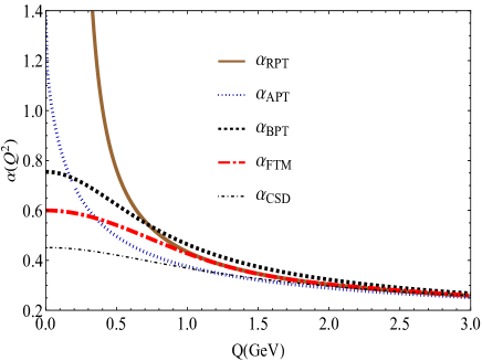
Figure 1: QCD running coupling constant versus renormalization scale for different models.

II.1 Thermodynamic potential

The system under study is the SQM composed of up, down, and strange quark flavors at zero temperature and finite chemical potential. The masses of the up and down quarks are negligible. However, for the strange quark, the running mass with the value of $0.95_{-3}^{+9}MeV$ $\cong 0.1GeV$ in $Q=2GeV$ Zyla2020 is considered (see Eq. 6). Since the QED interactions between quarks and the interactions between gravitons are negligible compared to the QCD interaction, QCD is the dominant interaction in the system. By knowing the thermodynamic potential of the system, the properties of the SQM, such as energy density, quark number density, pressure, sound speed, adiabatic index, etc., can be derived. To obtain the thermodynamic potential ($\Omega$), it is divided into non-interacting and perturbative parts: i) the non-interacting or free part consists of non-interacting quarks and electrons; ii) the perturbative part consists of the QCD interactions between the quarks. The perturbative part has been previously obtained through two- and three-loop Feynman diagrams up to the first and second order of the coupling constant, in Refs. Fraga2006 and Kurkela2010 , respectively. The thermodynamic potential of a quark flavor with mass $m$ up to leading order is as follows Kurkela2010

$$-\frac{\Omega}{V}=\sum_{{N_{f}=1}}^{3}\left({\mathcal{M}}_{1}+\frac{{\mathcal{M}}_{2}\alpha_{s}(Q)}{4\pi}\right),$$ (3)

where ${\mathcal{M}}_{1}$ and $\frac{{\mathcal{M}}_{2}\alpha_{s}(Q)}{4\pi}$ are non-interacting and perturbative parts, respectively. ${\mathcal{M}}_{1}$ and ${\mathcal{M}}_{2}$ are as follows

$${\mathcal{M}}_{1}=\frac{N_{c}\mu^{4}}{24\pi^{2}}\bigg{\{}2\hat{u}^{3}-3z\hat{m}^{2}\bigg{\}},$$ (4)

$${\mathcal{M}}_{2}=\frac{d_{A}\mu^{4}}{4\pi^{2}}\Bigg{\{}-6z\hat{m}^{2}\ln\frac{Q}{m}+2\hat{u}^{4}-4z\hat{m}^{2}-3z^{2}\Bigg{\}},$$ (5)

where, $\hat{u}\equiv(\sqrt{\mu^{2}-m^{2}})/\mu$, $\hat{m}\equiv m/\mu$, $z\equiv\hat{u}-\hat{m}^{2}\,\ln\bigg{[}\frac{1+\hat{u}}{\hat{m}}\bigg{]}$ and $d_{A}\equiv N^{2}_{c}-1$. As we mentioned, we consider up and down quarks massless. The running mass of the strange quark is Kurkela2010

$$m(Q)=m(2GeV)\left(\frac{\alpha_{s}(Q)}{\alpha_{s}(2GeV)}\right)^{\gamma_{0}/\beta_{0}},$$ (6)

where $\gamma_{0}\equiv 3\frac{N_{c}^{2}-1}{2N_{c}}$ and $\beta_{0}\equiv\frac{11N_{c}-2N_{f}}{3}$. Moreover, we have considered $m(2GeV)\simeq 0.1GeV$ and $\alpha_{s}(2GeV)\simeq 0.3$ Zyla2020 . The pressure is derived from the relation $P=-B-\frac{\Omega}{V}$, where $V$ is the volume of the system. It is notable that $B$ is a free parameter considered for all non-perturbative effects not included in the perturbative expansion Kurkela2010 . The values of $B$ are obtained in such a way to get zero total pressure at the surface of the star where the baryon number density is minimum Kurkela2010 ; sedaghat2022plb . Therefore the B parameter corresponds to the onset density (see tables 3 and 4). If the perturbative interaction between the quarks is neglected, $B$ will have the role of the bag constant in the system. The renormalization scale $Q$ appears in pressure through the running mass of the strange quark and the running coupling constant. At finite temperature $(T)$ and finite chemical potential $(\mu)$, the phenomenological models suggest $Q=2\pi\sqrt{T^{2}+\frac{\mu^{2}}{\pi^{2}}}$ for a massless quark. At zero temperature with $N_{f}$, $Q=2\left({\ \sum_{f}\mu_{f}/3}\right)\equiv 2\overline{\mu}$ which can vary by a factor of $2$ with respect to its central value Schneider2003 ; Karmakar2019 ; Bandyopadhyay2019 . Employing all the required constraints for SQM (charge neutrality, beta equilibrium, $\epsilon/nB<0.930MeV$, and $n_{s}>0$), we obtain the EOS for SQS.

II.2 Stability conditions and EOSs

After calculating the thermodynamic potential, the EOSs of the stable SQSs can be obtained from the following relation

$$\varepsilon=-\left(P_{u}+P_{d}+P_{s}\right)+\mu_{u}n_{u}+\mu_{d}n_{d}+\mu_{s}n_{s},$$ (7)

where $\varepsilon$, $P_{i}$, $\mu_{i}$ and $n_{i}$ are the energy density, pressure, chemical potential, and quark number density with flavor $i$, respectively. It should be noted that to calculate the EOSs, the charge neutrality and beta equilibrium constraints have to be imposed Blaschke2001 . As a result, $\mu_{s}=\mu_{d}\equiv\mu,\leavevmode\nobreak\ \mu_{u}=\mu-\mu_{e},\leavevmode\nobreak\$and$\leavevmode\nobreak\ 2n_{u}/3-n_{d}/3-n_{s}/3-n_{e}=0$ hold where $n_{e}=eB\mu_{e}^{2}/(2\pi)^{2}$is the electron number density. Another constraint is that the minimum energy density per baryon number density should be lower than that of the most stable nucleus (${}^{56}Fe$) Witten1984 ; Terazawa1989 ; Weber2005 , i.e. $\varepsilon/n_{B}\leq 0.93GeV$ where $n_{B}$ is the baryon number density and is equals $n_{B}=\left(n_{u}+n_{d}+n_{s}\right)/3$. The minimum value of $n_{B}$ corresponds to the point that the strange quark number density is non-zero provided that the constraint for the minimum energy density per baryon is satisfied and the perturbative expansions of the pressures and the quark number densities are not broken down.

II.3 Thermodynamic properties of SQM in BPT and APT models

Here, the results for the EOSs of SQM in the APT and BPT models are presented. First, the critical baryon number density ($n_{cr}$) at which SQM begins to appear should be obtained. For this purpose, the minimum value of $n_{B}$ is calculated. For this value, the perturbative expansion must be valid, and the constraints of the SQM must be satisfied. The obtained baryon number density is referred to as the minimum critical baryon number density and is denoted by $(n_{cr})_{min}$. The value of $n_{cr}$ must be more than $(n_{cr})_{min}$ because the higher order contributions (compared with the leading order) in the perturbative expansion are ignored. Table. 1, shows the values of $(n_{cr})_{min}$ in the RPT, APT and BPT models for different values of the renormalization scale. As one can see from Table. 1, the $(n_{cr})_{min}$ of the APT and BPT models is obtained at lower energies than that of the RPT model. This feature is due to the behavior modification of the coupling constant in the IR region in the APT and BPT models. Moreover, there is little difference between the $(n_{cr})_{min}$ values of the APT, and BPT models. This stems from the fact that the $(n_{cr})_{min}$ values are obtained at $Q\gtrsim 0.8GeV$ where the coupling constants in the APT and BPT models behave almost similarly (see figure. 1). According to Table. 1, the value of $(n_{cr})_{min}$ for the APT and BPT models is about $0.1fm^{-3}$. As mentioned above, $n_{cr}>(n_{cr})_{min}$ values must be used. Using bag models in Refs. Sagert2009 and Sagert2010 , $n_{cr}$ was obtained in the interval $0.1fm^{-3}\lesssim n_{cr}\lesssim 0.5fm^{-3}$. By setting $Q=4\overline{\mu}$, different values of $n_{cr}\geq(n_{cr})_{min}$ are selected to obtain EOSs, and consequently, the maximum gravitational masses of SQSs in the APT and BPT models. It is noteworthy that the maximum gravitational masses are decreased by increasing $n_{cr}$.

Table 1: Minimum values of baryon number density $(n_{cr})_{min}$ for the strange quark matter by considering $Q=4\overline{\mu}$ in various models.

$RPT$	$RPT$	$APT$	$APT$	$BPT$	$BPT$
$\overline{\mu}$	$(n_{cr})_{min}$	$\overline{\mu}$	$(n_{cr})_{min}$	$\overline{\mu}$	$(n_{cr})_{min}$
(MeV)	($fm^{-3}$)	(MeV)	($fm^{-3}$)	(MeV)	($fm^{-3}$)
278	0.154	236	0.099	245	0.097

In Figure. 2, the EOSs of SQM in the APT and BPT models are presented for different values of $n_{cr}$. Each color corresponds to a different $n_{cr}$. In both models, the EOSs become softer when $n_{cr}$ increases.

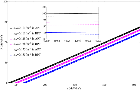
Figure 2: EOSs of SQM in APT and BPT models for different choices of $n_{cr}$. Continuous and dashed lines correspond to APT and BPT models, respectively. Each color indicates a $n_{cr}$ as follows. Continuous and dashed black lines correspond to $n_{cr}=0.101fm^{-3}$, continuous and dashed magenta lines correspond to $n_{cr}=0.128fm^{-3}$, and continuous and dashed blue lines correspond to $n_{cr}=0.155fm^{-3}$.

It is worthwhile to mention that the EOSs should satisfy the conditions of causality and dynamic stability. To meet the causality condition, the speed of sound ($c_{s}=\sqrt{dP/d\epsilon}$) should be lower than the speed of light in vacuum ($c_{s}\leq 1$). Figure. 3, shows the behavior of $c_{s}^{2}$ versus energy density for different values of $n_{cr}$. Based on some arguments in the perturbation theory, $c_{s}^{2}$ should approach $1/3$ from below at asymptotically large densities Tan2020 . Figure. 3, indicates that this behavior is well satisfied in our EOSs for both APT and BPT models.

To satisfy the dynamic stability condition, the value of the adiabatic index $\left(\Gamma=\frac{(P+\epsilon)dP}{Pd\epsilon}\right)$ should be higher than $4/3$ Chandrasekhar1964 ; Bardeen1966 ; Kuntsem1988 ; Mak2013 ; Eslam2017 . This constraint holds for our EOSs in both APT and BPT models. Figure. 4, shows that the adiabatic index of SQM versus energy density is higher than 4/3 for all $n_{cr}$ values used in both APT and BPT models. It is worth mentioning that the constraints $\epsilon+P\geq 0$ and $\epsilon\geq\left|P\right|$ Hendi2016 ; Hendi2017 ; EslamPanah2019b ; Roupas2021 are well satisfied in our calculations as well.

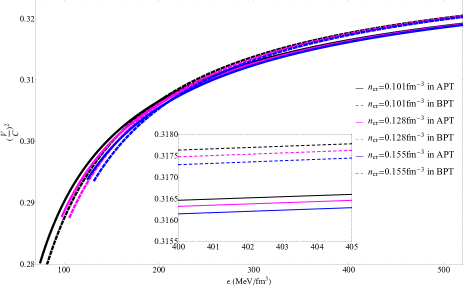
Figure 3: Squared sound velocity versus energy density in APT and BPT models for different choices of $n_{cr}$. Continuous and dashed lines correspond to APT and BPT models, respectively. Each color indicates a $n_{cr}$ as follows. Continuous and dashed black lines correspond to $n_{cr}=0.101fm^{-3}$, continuous and dashed magenta lines correspond to $n_{cr}=0.128fm^{-3}$, and continuous and dashed blue lines correspond to $n_{cr}=0.155fm^{-3}$.

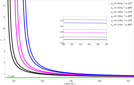
Figure 4: Adiabatic index in APT and BPT models for different choices of $n_{cr}$. Continuous and dashed lines correspond to APT and BPT models, respectively. Each color indicates a $n_{cr}$ as follows. Continuous and dashed black lines correspond to $n_{cr}=0.101fm^{-3}$, continuous and dashed magenta lines correspond to $n_{cr}=0.128fm^{-3}$, and continuous and dashed blue lines correspond to $n_{cr}=0.155fm^{-3}$.

II.4 Calculation of the remnant masses of non-rotating and rapidly-rotating compact stars

The gravitational wave (GW) observations give the total gravitational mass of the binary system with the assumption that its components are at an infinite distance from each other Gao2020 . In order to obtain the remnant mass of a binary NS merger, the total baryonic mass must first be calculated from the total gravitational mass through the conversion relations shown in Table. 2 Lattimer1989 ; Timmes1996 ; Coughlin2017 ; Gao2020 . As one can see from Table. 2, there are some conversion relations between baryonic mass ($M_{b}$) and gravitational mass ($M_{g}$) for NR and rapidly rotating (RR) NSs. After calculating the total baryonic mass from components of the binary, the mass ejected during the merger is deduced from it. Hence, the remnant baryonic mass is obtained and converted back to the remnant gravitational mass. Before the merger, the low-spin approximation is assumed for the components in the binary system. Therefore, the conversion relations are used for NR stars. There is a different scenario for the remnant mass. Since the remnant mass must be rapidly spinning, the RR conversion relations between $M_{b}$ and $M_{g}$ are used Gao2020 . The first and last relations in Table. 2 are used as the conversion relations for the phases before and after the merger, respectively. Assuming the maximum expected value of the mass ejected for GW190425 ($M_{ejecta}=0.04{M}_{\odot}$ Foley2020 ), the remnant mass of GW190425 is obtained in the range of $3.11-3.54{M}_{\odot}$. It should be noted that in the calculations, the mass ratio of the binary GW190425 is bound to $0.4-1$ Abbott2020ApJL . The remnant might require the EOS at non-zero temperature and out of beta equilibrium Khadkikar2021 , and consequently, the universal relations at finite temperature are needed N.khosravi2021 . But it depends on the star’s state and the system’s Fermi temperature. For the strong shocks at the merger, the temperature of the merged stellar object can reach up to $30-50MeV$ L.Baiotti2017 . However, the star’s temperature will be rapidly reduced by neutrino emission L.Baiotti2017 . On the other hand, the Fermi temperature of quark stars is several times the Fermi temperature of neutron stars. As we know, the Fermi energy at zero temperature is equivalent to the chemical potential. Table 1 shows that the lowest value for the Fermi energy is about $240MeV$. While in a neutron star at saturation density, this value is about 50$MeV$. Therefore, the finite temperature effects can be considerable for the newborn neutron stars Khadkikar2021 .

Table 2: Relation between total baryonic mass and total gravitational mass for NR and RR stars. Below each relation, there are two numbers as the maximum residual error (outside the parenthesis) and the average residual error (inside the parenthesis).

NR NSs	RR NSs
$M_{b}=Mg+0.075M_{g}^{2}$	$M_{b}=Mg+0.064M_{g}^{2}$
$5.8\%(1.5\%)$	$3.3\%(1.2\%)$
Timmes1996	Gao2020
$M_{b}=Mg+0.084M_{g}^{2}$	$M_{b}=Mg+0.073M_{g}^{2}$
$4.1\%(1.7\%)$	$6.0\%(1.6\%)$
Lattimer1989	Gao2020
$\frac{M_{b}}{M_{g}}=1+0.89(\frac{M_{g}}{R})^{1.2}$	$M_{b}=Mg+.056M_{g}^{2}+0.002M_{g}^{3}$
$2.6\%(0.56\%)$	$4.0\%(0.95\%)$
Coughlin2017	Gao2020

III SQS structure

Using the computed EOSs in section C, the maximum gravitational mass can be obtained by solving the TOV equation Tolman1939 ; Oppenheimer1939 . The results for the APT and BPT models have been presented in Tables. 3 and 4, and also figures. 5 and 6. The limiting behavior of the mass in Figure 5 shows the maximum gravitational mass of SQS. From this figure, we can obtain the range of energy density for SQS. In Ref. Kurkela2010 , the maximum gravitational mass of SQS has been obtained as $M\simeq 2.75{M}_{\odot}$ by using the RPT model. Our results in the APT model for $(n_{cr})_{min}=0.101fm^{-3}$ and $n_{cr}=0.128fm^{-3}$ are considerably larger than that in Kurkela2010 . This indicates the great importance of the IR behavior of the running coupling constant in the structure of a quark star. It is notable that the maximum gravitational masses obtained in our models are outside the limits obtained by observational constraints for neutron stars (such as GW170817 Rezzolla2018 ; Shibata2019 ). Such a violation motivates us to study the remnant mass of GW190425 as a strange quark star. However, the two-families scenario Alessandro Drago (neutron stars and strange quark stars coexist) allows the existence of massive quark stars without refuting observational arguments. Furthermore, the compact object with the mass $2.5-2.67M_{\odot}$ in GW190814 is expected to be a strange quark star Zhiqiang Miao . In Ref. I.Bombaci2021 , this object is investigated as a SQS within the two-families scenario. There are different colored regions in Figure. 6. The blue region shows the remnant mass of GW190425 obtained in section D. In the current study, the maximum gravitational mass for the RR SQS represented by the horizontal green region ranged from $3.02-3.94$${M}_{\odot}$. The vertical green region, which represents the corresponding radius of the maximum mass of the RR SQSs ranges from 14.14$km$ to $18.52$$km$ in our calculations. Finally, the black hatched region, the common region between the two mentioned green regions, shows our results for the RR SQSs. As can be observed in Fig. 6, this region completely covers the remnant mass of GW190425.

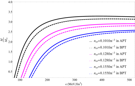
Figure 5: Mass versus energy density in APT and BPT models for different choices of $n_{cr}$. Continuous and dashed lines correspond to APT and BPT models, respectively. Each color indicates a $n_{cr}$ as follows. Continuous and dashed black lines correspond to $n_{cr}=0.101fm^{-3}$, continuous and dashed magenta lines correspond to $n_{cr}=0.128fm^{-3}$, and continuous and dashed blue lines correspond to $n_{cr}=0.155fm^{-3}$.

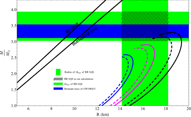
Figure 6: $M$-$R$ of SQSs in the APT and BPT models for different choices of $n_{cr}$. The blue region is related to the remnant mass of GW190425. The horizontal and vertical green regions show intervals of maximum mass of RR SQSs and corresponding radii, respectively. The black hatched region is related to our results for maximum masses and corresponding radii of RR SQSs. Continuous and dashed lines correspond to different $n_{cr}$, which are the same as the ones in Figures. 2, 3 and 4.

Table 3: The structural properties of the NR and RR SQSs in the APT model for different values of $n_{cr}$. It is notable that indices NR and RR, are related to NR and RR SQSs.

$n_{cr}$	$M_{TOV}$	$R_{NR}$	$M_{max_{RR}}$	$M_{B_{NR}}$	$R_{Sch_{NR}}$	$z_{NR}$	${\color[rgb]{0,0,0}B}$
$fm^{-3}$	$({M}_{\odot})$	$(km)$	$({M}_{\odot})$	$({M}_{\odot})$	$(km)$		${\color[rgb]{0,0,0}\frac{MeV}{(fm)^{3}}}$
0.101	3.28	18.52	3.94	5.58	9.67	0.45	15.23
0.128	2.90	16.80	3.48	5.06	8.55	0.43	20.31
0.155	2.59	14.52	3.11	4.37	7.64	0.45	26.39

Table 4: The structural properties of the NR and RR SQSs in the BPT model for different values of $n_{cr}$.

$n_{cr}$	$M_{TOV}$	$R_{NR}$	$M_{max_{RR}}$	$M_{B_{NR}}$	$R_{Sch_{NR}}$	$z_{NR}$	${\color[rgb]{0,0,0}B}$
$fm^{-3}$	$({M}_{\odot})$	$(km)$	$({M}_{\odot})$	$({M}_{\odot})$	$(km)$		${\color[rgb]{0,0,0}\frac{MeV}{(fm)^{3}}}$
0.101	3.15	17.62	3.78	5.31	9.29	0.45	19.84
0.128	2.80	15.61	3.36	4.70	8.26	0.46	25.09
0.155	2.52	14.14	3.02	4.26	7.43	0.45	31.03

Now, it is explained how to calculate the maximum gravitational masses of the RR SQSs in the APT and BPT models. As was mentioned in section D, the remnant mass must be rapidly-rotating. If the rapidly-rotating remnant mass loses its centrifugal support, it will collapse into a BH Sarin2020 . To obtain the maximum mass of the rotating SQSs, the universal relation derived in Ref. Breu2016 was used. They used $15$ nuclear-physics EOSs for NR and RR compact stars and obtained a universal relation between the maximum mass of a uniformly rotating star ($M_{max_{RR}}$) and the maximum mass of the NR star obtained by TOV equation $(M_{TOV})$.

$$M_{max_{RR}}=(1.203\pm 0.022)M_{TOV}.$$ (8)

As we mentioned, this universal relation has been obtained by nucleonic EoSs. It is notable that the authors of Ref. Breu2016 have also suggested the universal relation $M_{max_{RR}}=1.44M_{TOV}$ for SQSs. But they have noted that additional work is needed to confirm this behavior. Therefore, we have not used this relation in our paper. However, if we use this universal relation, our results would cover better the remnant mass of GW190425.

The result is a horizontal green region in Figure. 6, which ranges from $3.02-3.94$${M}_{\odot}$. It is noteworthy that considering anisotropic models for the quark star can even increase the mass up to $5M_{\odot}$ J.Horvath .

It has previously been shown that when the causality and Le Chatelier principles are used in GR, the mass of a NS cannot be larger  than $3.2M_{\odot}$ Rhoades1974 . Therefore, the remnant mass of GW190425 is not expected to be a NS. Moreover, the upper mass limit of a static spherical star with a uniform density in GR is given by $M_{B}=\frac{4c^{2}R}{9G}$ (the Buchdahl theorem) Buchdahl1959 . According to this compactness limit, a boundary between a BH and a star can be determined. Indeed, for $M_{max}<M_{B}$, the compact object cannot be a BH. In other words, the results show that the maximum masses of the compact objects in the current study are less than the mass of the Buchdahl limit. Hence, these massive compact objects are not BHs (see Tables. 3 and 4). In addition, the radii of these compact objects are more than the Schwarzschild radius $\left(R>R_{Sch}=\frac{2GM}{c^{2}}\right)$ and the obtained redshifts are less than $1$ $\left(z=\frac{1}{\sqrt{1-\frac{2GM}{c^{2}R}}}-1<1\right)$ (see Tables. 3 and 4). These results ensure that these compact objects are not BHs or NSs. As a result, RR SQSs may have masses larger than $3.2M_{\odot}$. Therefore, the remnant mass of GW190425 may be considered a SQS.

IV Summary and Conclusion

In this paper, the EOSs of SQSs were calculated in the leading order of $\alpha_{s}$ by using the APT and BPT models. It is known that the constant coupling behavior of the QCD is a challenging issue. Unlike the RPT model in which the coupling constant is infinite at IR momenta, the employed models in this paper have finite values at all energy scales for the running coupling constant. Considering a compact star as a large laboratory to probe the QCD models, the EOSs in GR were used in order to investigate the structural properties of SQSs at zero temperature. We had not made any assumptions about the onset density of the quark matter. Rather, we obtained it by perturbative calculations. By employing a set of equations coming from the chemical equilibrium and the charge neutrality conditions and also imposing the constraints for SQM ($\epsilon/n_{B}<930MeV\ \&\ n_{s}>0$), we showed that the SQM phase could occur at $n_{B}<0.16fm^{-3}$ in leading order perturbation theory. We found the minimum value for onset density of SQM as $0.1fm^{-3}$. One should note that we study the matter inside a compact star or the matter after merging two neutron stars, which has completely different conditions than the usual conditions in laboratories. It is worth mentioning that in RefSagert2009 , the onset densities have been considered to be around $0.1fm^{-3}$ for stars with proton fractions $Y_{p}<0.3$. However, one might say that the onset density of the quark matter might be greater than the value obtained from the leading order perturbative calculations, and considering the higher-order terms in perturbation leads to higher values for onset density of SQM. For this issue, we have also used other values of onset density of SQM, including 0.128 $fm^{-3}$ and $0.155fm^{-3}$. Then, we obtained the maximum gravitational masses of SQSs in APT and BPT models, which were considerably larger than that of the RPT model. By using the component masses of GW190425 as well as some conversion relations between the baryonic mass and the gravitational mass, the remnant mass of GW190425 was obtained. Our results for the maximum gravitational mass of SQS were comparable with the remnant mass of GW190425. Then, the obtained gravitational masses were modified by considering the effect of the star’s rotation on them. In this way, the results completely covered the remnant mass of GW190425 and showed that the remnant mass of GW190425 might be a SQS. Our results corresponded to three different onset densities including $0.101fm^{-3}$, $0.128fm^{-3}$ and $0.155fm^{-3}$. Even if we ignore our calculations corresponding to the onset density $0.101fm^{-3}$, our results still fall within the range of the remnant mass of GW190425 (we have obtained the remnant mass of GW190425 in the range $3.11-3.54M_{\odot}$). As tables 3 and 4 of the paper Show, for the onset density $0.128fm^{-3}$ ($Q>1.01GeV$), the maximum mass of SQS is $3.48M_{\odot}$ and $3.36M_{\odot}$ in APT and BPT models, respectively. Here, it can be asked the question of why we compared our results with the remnant mass of GW190425. As the post-merger of GW190425 falls within the unknown mass gap region ($2.5-5M_{\odot}$), its nature is ambiguous. Given the remnant mass of GW190425 $(3.11-3.54M_{\odot})$, it is unlikely to be a supermassive neutron star. Hence it may be a black hole or a quark star. Our calculations suggest that the remnant mass of GW190425 may be a strange quark star. In addition, if a pulsar falls within the range of the obtained masses and radii, it is likely to be a strange quark star.

Appendix A: Deriving the analytic coupling constant at one-loop approximation

Using the Källén-Lehman spectral representation, the analytic coupling constant ($\alpha_{an}$) is defined as Shirkov1997

$$\alpha_{APT}=\frac{1}{\pi}\int_{0}^{\infty}d\sigma\frac{\rho(\sigma,a)}{\sigma+Q^{2}-i\epsilon},$$ (9)

where $\rho(\sigma,a)=Im(\alpha_{RG}(-\sigma-i\epsilon,a))$ is the spectral density function calculated by the imaginary part of $\alpha_{RG}$ (the running coupling constant obtained from the renormalization group equations). The spectral density function at one-loop approximation is given by

$$\rho(\sigma,a)=\frac{a^{2}\beta_{0}\pi}{\left(1+a\beta_{0}\ln\sigma/\mu^{2}\right)^{2}+(a\beta_{0}\pi)^{2}}.$$ (10)

By inserting Eq. (10) in Eq. (9), we get

$$\alpha_{APT}^{(1)}=\frac{4\pi}{\beta_{0}}\left[\left(\ln\left(\frac{Q^{2}}{\Lambda^{2}}\right)\right)^{-1}+\frac{\Lambda^{2}}{\Lambda^{2}-Q^{2}}\right].$$ (11)

Appendix B: The running coupling constant in BPT

The running coupling constant derived from BPT Simonov1995 ; Badalian1997 ; Simonov2011 is based on the success of static potential $q\overline{q}$ in which the QCD interaction is divided into two parts as $V(r)=-\frac{4\alpha_{V}}{3r}+\sigma r$. In this equation, the first term is the perturbative part for short-distance interactions and the second term is the non-perturbative part for the long-distance interactions. In the BPT model, the gluon field is divided into perturbative and non-perturbative parts. The non-perturbative part is a background field which is described by the QCD string tension ($\sigma$). To avoid the $\Lambda$ pole problem, an effective gluonic mass ($m_{2g}^{2}=2\pi\sigma$) is assumed to be produced by this non-perturbative background field Simonov2011 . The IR behavior of the running coupling constant is then modified by adding this non-perturbative part to all gluonic logarithms ($\ln Q^{2}\longmapsto\ln(Q^{2}+m_{2g}^{2})$) at all loop orders. At one-loop approximation, the following equation is obtained

$$\alpha_{BPT}^{(1)}(Q^{2})=\frac{4\pi}{\beta_{0}}\left(\ln\left(\frac{Q^{2}+m_{2g}^{2}}{\Lambda^{2}}\right)\right)^{-1},$$

where, $\Lambda$ is $0.480$$GeV$.

Appendix C: Structural properties of SQS in APT model for different values of renormalization scale.

As we mentioned in the introduction section, at zero temperature the phenomenological models suggest $Q=[1\overline{\mu}-4\overline{\mu}](\overline{\mu}\equiv\sum_{f}\mu_{f}/3)$. We set the maximum value for $Q$ ($Q=4\overline{\mu}$) to find the maximum possible mass of the SQS in our models and minimize the confinement effects. However we found that for $Q\gtrsim 3.4\overline{\mu}$ the results do not change considerably, especially for $n_{cr}=0.128fm^{-3}$ and $n_{cr}=0.155fm^{-3}$. Figure. 7 and Table. 5 show this feature for two different values of $Q$, including $Q=3.4\overline{\mu}$ and $Q=4\overline{\mu}$. We have defined $\delta_{M}\equiv\frac{M_{4\overline{\mu}}-M_{3.4\overline{\mu}}}{(M_{4\overline{\mu}}+M_{3.4\overline{\mu}})/2}$ and $\delta_{R}\equiv\frac{R_{4\overline{\mu}}-R_{3.4\overline{\mu}}}{(R_{4\overline{\mu}}+R_{3.4\overline{\mu}})/2}$ as a measure to see the difference of structural features in two different renormalization scales. As the Table. 5 shows, the values of $\delta_{M}$ and $\delta_{R}$ are less than $5\%$. Specifically, the values of these quantities for $n_{cr}=0.128fm^{-3}$ and $n_{cr}=0.155fm^{-3}$ are negligible.

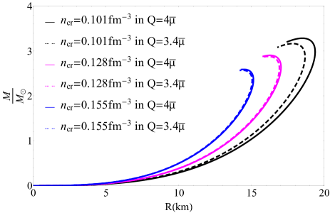
Figure 7: Mass versus radius of SQS in APT model for different choices of $Q$. Continuous and dashed lines correspond to $Q=4\overline{\mu}$ and $Q=3.4\overline{\mu}$, respectively. Each color indicates a $n_{cr}$ as follows. Continuous and dashed black lines correspond to $n_{cr}=0.101fm^{-3}$, continuous and dashed magenta lines correspond to $n_{cr}=0.128fm^{-3}$, and continuous and dashed blue lines correspond to $n_{cr}=0.155fm^{-3}$.

Table 5: Structural properties of SQS for different values of $Q$

	$Q/\overline{\mu}=3.4$		$Q/\overline{\mu}=4$		%
$n_{cr}(fm^{-3})$	$M(M_{\odot})$	$R(km)$	$M(M_{\odot})$	$R(km)$	$\delta_{M}$	$\delta_{R}$
$0.101$	$3.16$	$17.74$	$3.28$	$18.52$	$3.73$	$4.30$
$0.28$	$2.88$	$16.14$	$2.90$	$16.80$	$0.69$	$2.41$
$0.155$	$2.57$	$14.45$	$2.59$	$14.52$	$0.77$	$0.48$

References

- (1) B. P. Abbott, et al., Astrophys. J. Lett. 892, L3 (2020).
- (2) G. M. Prosperi, M. Raciti, and C. Simolo, Prog. Part. Nucl. Phys. 58, 387 (2007).
- (3) G. Altarelli, [arXiv:1303.6065].
- (4) A. Deur, S. J. Brodsky, and G. F. de Teramond, Prog. Part. Nucl. Phys. 90, 1 (2016).
- (5) A. Deur, V. Burkert, J. P. Chen, and W. Korsch, Phys. Lett. B 665, 349 (2008).
- (6) R. Perez-Ramos, V. Mathieu, and M. -A. Sanchis-Lozano. JHEP 10, 47 (2010).
- (7) OPAL Collaboration, Euro. Phys. J. C 7, 571 (1999).
- (8) S. J. Brodsky, S. Menke, C. Merino, and J. Rathsman, Phys. Rev. D 67, 055008 (2003).
- (9) S. J. Brodsky, and R. Shrock, Phys. Lett. B 666, 95 (2008).
- (10) G. S. Bali, Phys. Rep. 343, 1 (2001).
- (11) C. S. Fischer, J. Phys. G Nucl. Phys. 32, R253 (2006).
- (12) D. Zwanziger, Phys. Rev. D 65, 094039 (2002).
- (13) A. C. Mattingly, and P. M. Stevenson, Phys. Rev. Lett. 69, 1320 (1992).
- (14) J. A. Gracey, JHEP 06, 052 (2006).
- (15) A. M. Badalian, and Yu. A. Simonov, Phys. At. Nucl. 60, 630 (1997).
- (16) Yu. A. Simonov, Phys. At. Nucl. 74, 1223 (2011).
- (17) D. V. Shirkov, and I. L. Solovtsov, Phys. Rev. Lett. 79, 1209 (1997).
- (18) G. S. Bali, et al., Nucl. Phys. B Proc. Suppl. 153, 9 (2006).
- (19) V. Gribov, Euro. Phys. J. C 10, 71 (1999).
- (20) N. Farrow, X. -J. Zhu, and E. Thrane, Astrophys. J. 876, 18 (2019).
- (21) K. Kyutoku et al., Astrophys. J. Lett. 890, L4 (2020).
- (22) I. M. Romero-Shaw, N. Farrow, S. Stevenson, E. Thrane, and X. -J. Zhu, MNRAS. Lett. 496, L64 (2020).
- (23) M. -Z. Han et al., Astrophys. J. Lett. 891, L5 (2020).
- (24) V. Korol, and M. Safarzadeh, MNRAS 502, 5576 (2021).
- (25) S. Clesse, and J. Garcia-Bellido, [arXiv:2007.06481].
- (26) B. Eslam Panah, T. Yazdizadeh, and G. H. Bordbar, Eur. Phys. J. C 79, 815 (2019).
- (27) R. Nandi and P. Char, Astrophys. J. 857, 12 (2018).
- (28) J. J. Li, A. Sedrakian, and M. Alford, Phys. Rev. D 104, L121302 (2021).
- (29) A. Kurkela, P. Romatschke, and A. Vuorinen, Phys. Rev. D 81, 105021 (2010).
- (30) A. M. Badalian and A. I. Veselov, Physics of Atomic Nuclei. 68, 582 (2005).
- (31) R. A. Schneider, [arXiv:hep-ph/0303104].
- (32) B. Karmakar, R. Ghosh, A. Bandyopadhyay, N. Haque, and M. G. Mustafa, Phys. Rev. D 99, 094002 (2019).
- (33) A. Bandyopadhyay, B. Karmakar, N. Haque, and M. G. Mustafa, Phys. Rev. D 100, 034031 (2019).
- (34) A. Worley, P. G. Krastev, and B. -A. Li, Astrophys. J. 685, 390 (2008).
- (35) C. Breu, and L. Rezzolla, MNRAS 459, 646 (2016).
- (36) S. Godfrey, and N. Isgur, Phys. Rev. D 32, 189 (1985).
- (37) J. M. Cornwall, Phys. Rev. D 26, 1453 (1982).
- (38) Yu. A. Simonov, Phys. At. Nucl. 58, 107 (1995).
- (39) A. M. Badalian, and B. L. G. Bakker, Phys. Rev. D 100, 054036 (2019).
- (40) P. A. Zyla et al. (Particle Data Group), Prog. Theor. Exp. Phys. 2020, 083C01 (2020).
- (41) E. S. Fraga, Nucl. Phys. A 774, 819 (2006).
- (42) D. Blaschke, N. K. Glendenning, and A. Sedrakian, (Ed.), Physics of neutron star interiors, Germany: Springer (2001).
- (43) J. Sedaghat, S. M. Zebarjad, G. H. Bordbar, B. Eslam Panah, Phys. Lett. B 829, 137032 (2022).
- (44) E. Witten, Phys. Rev. D 30, 272 (1984).
- (45) H. Terazawa, J. Phys. Soc. Jpn. 58, 3555 (1989).
- (46) F. Weber, Prog. Part. Nucl. Phys. 54, 193 (2005).
- (47) I. Sagert et al., Phys. Rev. Lett. 102, 081101 (2009).
- (48) I. Sagert et al., J. Phys. G: Nucl. Part. Phys. 37, 094064 (2010).
- (49) H. Tan, J. Noronha-Hostler, and N. Yunes, Phys. Rev. Lett. 125, 261104 (2020).
- (50) S. Chandrasekhar, Astrophys. J. 140, 417 (1964).
- (51) J. M. Bardeen, K. S. Thorne, and D. W. Meltzer, Astrophys. J. 145, 505 (1966).
- (52) H. Kuntsem, MNRAS 232, 163 (1988).
- (53) M. K. Mak, and T. Harko, Eur. Phys. J. C 73, 2585 (2013).
- (54) B. Eslam Panah et al., Astrophys. J. 848, 24 (2017).
- (55) S. H. Hendi, G. H. Bordbar, B. Eslam Panah, and S. Panahiyan, JCAP 09, 013 (2016).
- (56) S. H. Hendi, G. H. Bordbar, B. Eslam Panah, and S. Panahiyan, JCAP 07, 004 (2017).
- (57) B. Eslam Panah, and H. L. Liu, Phys. Rev. D 99, 104074 (2019).
- (58) Z. Roupas, G. Panotopoulos, and I. Lopes, Phys. Rev. D 103, 083015 (2021).
- (59) H. Gao et al., Front. Phys. 15, 24603 (2020).
- (60) J. M. Lattimer, and A. Yahil, Astrophys. J. 340, 426 (1989).
- (61) F. X. Timmes, S. E. Woosley, T. A. Weaver, Astrophys. J. 457, 834 (1996).
- (62) M. Coughlin et al., Astrophys. J. 849, 12 (2017).
- (63) R. J. Foley et al., MNRAS 494, 190 (2020).
- (64) S. Khadkikar, A. R. Raduta, M. Oertel, and A. Sedrakian, Phys. Rev. C 103, 055811 (2021).
- (65) N. Khosravi et al., [arXiv:2112.10439]
- (66) L. Baiotti, and L. Rezzolla, Rep. Prog. Phys. 80, 096901 (2017)
- (67) R. C. Tolman, Phys. Rev. 55, 364 (1939).
- (68) J. R. Oppenheimer, and G. M. Volkoff, Phys. Rev. 55, 374 (1939).
- (69) L. Rezzolla, E. R. Most, and L. R. Weih, Astrophys. J. Lett. 852 L25 (2018).
- (70) M. Shibata, E. Zhou, K. Kiuchi, and S. Fujibayashi, Phys. Rev. D 100, 023015 (2019).
- (71) A. Drago, A. Lavagno, and G. Pagliara, Phys. Rev. D 89, 043014 (2014).
- (72) Z. Miao et al., Astrophys. J. Lett. 917 L25 (2021).
- (73) I. Bombaci et al., Phys. Rev. Lett. 126, 162702 (2021).
- (74) N. Sarin, P. D. Lasky, and G. Ashton, Phys. Rev. D 101, 063021 (2020).
- (75) J. Horvath, and P. H. R. S. Moraes, International Journal of Modern Physics D, 30, 2150016 (2021)
- (76) C. E. Rhoades, and R. Ruffini, Phys. Rev. Lett. 32, 324 (1974).
- (77) H. A. Buchdahl, Phys. Rev. 116, 1027 (1959).