Extending Neural P-frame Codecs for B-frame Coding

Abstract

While most neural video codecs address P-frame coding (predicting each frame from past ones), in this paper we address B-frame compression (predicting frames using both past and future reference frames). Our B-frame solution is based on the existing P-frame methods. As a result, B-frame coding capability can easily be added to an existing neural codec. The basic idea of our B-frame coding method is to interpolate the two reference frames to generate a single reference frame and then use it together with an existing P-frame codec to encode the input B-frame. Our studies show that the interpolated frame is a much better reference for the P-frame codec compared to using the previous frame as is usually done. Our results show that using the proposed method with an existing P-frame codec can lead to 28.5% saving in bit-rate on the UVG dataset compared to the P-frame codec while generating the same video quality.

1 Introduction

There are two types of frames in the video coding domain, Intra-frames and Inter-frames. Intra-frames (I-frames) are encoded/decoded independently of other frames. I-frame coding is equivalent of image compression. Inter-frames are encoded using motion compensation followed by residuals i.e. a prediction of an input frame is initially devised by moving pixels or blocks of one or multiple reference frames and then the prediction is corrected using residuals. Prediction is an essential task in inter-coding, for it is the primary way in which temporal redundancy is exploited. In the traditional paradigm of video coding [34, 41], motion vectors are used to model the motion of blocks of pixels between a reference and an input image [34]. In the neural video coding domain, dense optical flow is usually used to model individual pixels movements. In both cases, a warping is performed on references using motion vectors or optical flow to generate the prediction.

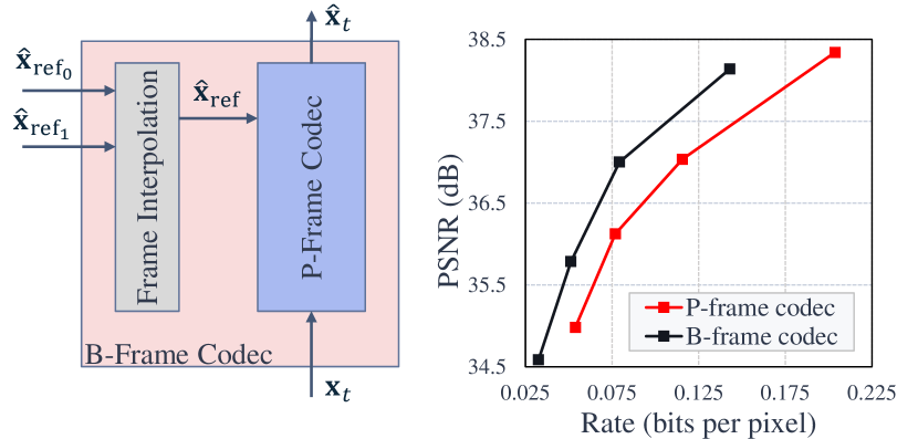
Figure 1: (a) the general idea of this work i.e. extending an existing P-frame codec to a B-frame codec by adding an interpolation block, (b) the rate-distortion improvements on the UVG dataset [38] where the P-frame [2] and the B-frame codecs are trained on the Vimeo-90k dataset [46] for the same number of iterations. The improvement is equivalent of 28.5% saving in bit-rate measured by BD-rate gain [6].

Inter-frames are further divided into Predicted (P) frames and Bi-directional predicted (B) frames. P-frame coding, which is suitable for low-latency applications such as video conferencing, uses only past decoded frames as references to generate a prediction. Most of the available literature on neural inter coding falls under this category and the methods often use a single past decoded frame as reference [23] (see Fig. 2.b). On the other hand, B-frame coding, which is suitable for applications such as on-demand video streaming, uses both past and future decoded frames as references. Future references provide rich motion information that facilitate frame prediction and eventually lead to better coding efficiency. The number of neural video codecs that address B-frame coding is limited [11, 13, 16, 43]. They use two references and generate a prediction either by bidirectional optical flow estimation and warping or by performing frame interpolation. The reported results show that these approaches, despite relative success in video coding, do not fully exploit the motion information provided by two references as the results are not competitive with state-of-the-art P-frame codecs [2].

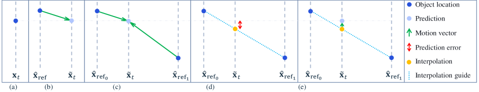
Figure 2: Prediction in inter-frame coding. $\mathbf{x}_{t}$, $\widetilde{\mathbf{x}}_{t}$, and $\widehat{\mathbf{x}}_{\textup{ref}}$ denote an input frame, the corresponding prediction and the reference, respectively. (a) Actual object location. (b) P-Frame prediction, a motion vector with respect to a single reference is transmitted. (c) B-frame prediction based on bidirectional flow/warp, two motion vectors with respect to two references are transmitted. (d) B-frame prediction based on frame interpolation, the interpolation result is treated as the prediction. No motion information is transmitted. (e) Our B-frame prediction approach, the interpolation result is corrected using a unidirectional motion vector similar to P-frame.

For a given input frame, when references from both past and future are available, under a linear motion assumption, one can come up with a rough prediction of the input frame by linearly interpolating the two references. This prediction does not need to be coded since the two references are already available to the receiver. The neural B-frame coding methods that work based on bidirectional flow/warping [13], do not use this useful information and send the optical flows with respect to both references (see Fig. 2.c). On the other hand, the interpolation outcome is only accurate under linear motion assumption. So in the neural B-frame models that rely on frame interpolation [11, 43], the prediction is likely to not exactly be aligned with the input frame (see Fig. 2.d). Even when a non-linear frame interpolator is employed [45], misalignment could still occur. In these situations, the codec solely relies on residuals to compensate for the misalignment. As a result, coding efficiency could be significantly lower compared to a scenario where the misalignment is mitigated via some inexpensive side-information first before applying residual coding.

In this work, we address this issue by introducing a new approach for neural B-frame coding, which despite its simplicity, is proven very effective. The method involves interpolating two reference frames to obtain a single reference frame, which is then used by a P-frame model to predict the current frame (see Fig. 1 and Fig. 2.e). A residual is applied to this prediction.

Our method takes advantage of the rich motion information available to the receiver by performing frame interpolation and does not suffer from the residual penalty due to misalignment. Since our B-frame coding solution operates based on a P-frame codec, an existing P-frame codec can be used to code B-frames. In fact, the same network can learn to do both P-frame coding as well as contributing to B-frame compression. In other words, by adding a frame interpolator to a P-frame codec, the codec is able to code both P-frames and B-frames. One can freely choose an existing interpolation and P-frame method when implementing our technique.

In video coding, videos are split into groups of pictures (GoP) for coding. The neural video codec that we develop in this work $\operatorname{B-EPIC}$ (B-Frame compression through Extended P-frame & Interpolation Codec) supports all frame types. Given that different frame types yield different coding efficiencies, it is crucial to choose the right frame type for the individual frames in a GoP. In this work, we look closely into GoP structure.

Our main contributions and findings are as follows:

• We introduce a novel B-frame coding approach based on existing P-frame codecs and frame interpolation,

• A single P-frame network is used for both P-frame and B-frame coding through weight-sharing,

• A thorough analysis of the effect of GoP structure on performance is provided,

• The proposed solution outperforms existing neural video codecs by a significant margin and achieves new state-of-the-art results.

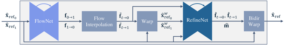
Figure 3: Frame interpolation method based on $\operatorname{Super-SloMo}$ [17]. $\operatorname{FlowNet}$ and $\operatorname{RefineNet}$ are trainable while $\operatorname{FlowInterpolation}$, $\operatorname{Warp}$, and $\operatorname{BidirWarp}$ are non-trainable operators. See section 3.1 for details.

2 Related work

I-frame/Image coding: Great progress has been made in the development of neural image codecs. Research has focused on various aspects of neural coding, such as architecture [3, 26, 30, 37], quantization [1], priors [5, 26], and multi-rate coding [12, 25, 36]. Recently, a hierarchical hyperprior model [4, 5] has been widely adopted in the neural coding field and there are multiple variants including some equipped with autoregressive models [27, 28] and attention mechanisms [10].

P-frame coding: Most of the existing neural video codecs fall under this category where unidirectional motion estimation/compensation is followed by residual correction [21, 22, 31]. Lu et al. introduced DVC [23], a basic P-frame codec which is later upgraded in [24]. While motion is often modelled using spatial optical flow, Agustsson et al. introduced scale-space flow [2] to address uncertainties in motion estimation via a blur field which is further enhanced in [47]. Recent works have introduced more sophisticated components, e.g. Golinski et al.  [15] added re currency to capture longer frame dependencies, Lin et al. look at multiple previous frames to generate a prediction in M-LVC [19], Liu et al. perform multi-scale warping in feature space in NVC [20], and Chen et al.  [9] replaced optical flow and warping by displaced frame differences.

B-frame coding: Wu et al.  [43] introduced one of the pioneering neural video codecs via frame interpolation that was facilitated by context information. Chang et al.  [11] improved the idea through adding a residual correction. Habibian et al.  [16] provided an implicit multi-frame coding solution based on 3D convolutions. Djelouah et al.  [13] employed bidirectional optical flow and warping feature domain residuals for B-frame coding. A recent work [29] provides a multi-reference video codec that could be applied to both P-frame and B-frame coding.

3 Method

We develop a neural video codec $\operatorname{B-EPIC}$ that consists of an I-frame codec, a P-frame codec, and a frame interpolator. The I-frame codec (Fig. 4.a) encodes individual frames $\mathbf{x}_{t}$ independently to produce a reconstruction $\widehat{\mathbf{x}}_{t}$. The P-frame codec applies a warp to a reference frame $\widehat{\mathbf{x}}_{\textup{ref}}$ to produce a prediction $\widetilde{\mathbf{x}}_{t}$ of $\mathbf{x}_{t}$, which is then corrected by a residual to obtain the reconstruction $\widehat{\mathbf{x}}_{t}$ (see Fig. 4.b). The frame interpolator takes two reference frames $\widehat{\mathbf{x}}_{\textup{ref}_{0}}$ and $\widehat{\mathbf{x}}_{\textup{ref}_{1}}$ and produces an interpolation $\widehat{\mathbf{x}}_{\textup{ref}}$ (see Fig. 3).

Our novel B-frame codec (Fig. 1) works by using the frame interpolator on references $\widehat{\mathbf{x}}_{\textup{ref}_{0}}$ and $\widehat{\mathbf{x}}_{\textup{ref}_{1}}$ to produce a single reference $\widehat{\mathbf{x}}_{\textup{ref}}$, which is then used by the P-frame codec to encode $\mathbf{x}_{t}$. The resulting system thus supports I-frames, P-frames and B-frames in a flexible manner.

Although our general method can be implemented using any frame interpolator and P-frame codec, in this work we develop a specific codec that uses the $\operatorname{Super-SloMo}$ [17] frame interpolator and the Scale-Space Flow ($\operatorname{SSF}$) codec [2]. The $\operatorname{SSF}$ P-codec is used within our video codec in a stand-alone fashion as well as in a B-frame codec when bundled with $\operatorname{Super-SloMo}$, while the two instances share weights. In the following subsections we discuss $\operatorname{Super-SloMo}$ and $\operatorname{SSF}$, as well as the GoP structure and loss function in more detail.

3.1 Frame interpolation

In the frame interpolation block, the goal is to interpolate two references whose time indices are normalized to $0$ and $1$, i.e. $\widehat{\mathbf{x}}_{\textup{ref}_{0}}$ and $\widehat{\mathbf{x}}_{\textup{ref}_{1}}$, to time $t$ where $0<t<1$. Since in B-frame coding, $\mathbf{x}_{t}$ could be anywhere between $\widehat{\mathbf{x}}_{\textup{ref}_{0}}$ and $\widehat{\mathbf{x}}_{\textup{ref}_{1}}$, an important factor in choosing $\operatorname{Super-SloMo}$ over other competitors is that $\operatorname{Super-SloMo}$ supports an arbitrary $t:\>0<t<1$ while many other methods assume $t=0.5$. The latter can be still used within our model, though they will impose restrictions on the GoP size. See section 3.3 for more details.

The block diagram of $\operatorname{Super-SloMo}$ is depicted in Fig. 3. $\operatorname{Super-SloMo}$ consists of two trainable components i.e. $\operatorname{FlowNet}$ and $\operatorname{RefineNet}$ as well as non-trainable $\operatorname{FlowInterpolation}$, $\operatorname{Warp}$, and $\operatorname{BidirWarp}$ blocks. Optical flow between $\widehat{\mathbf{x}}_{\textup{ref}_{0}}$ and $\widehat{\mathbf{x}}_{\textup{ref}_{1}}$ in the forward and backward directions, i.e. $\mathbf{f}_{0\rightarrow 1}$ and $\mathbf{f}_{1\rightarrow 0}$ where $\mathbf{f}_{0\rightarrow 1}$ denotes the optical flow from $\widehat{\mathbf{x}}_{\textup{ref}_{0}}$ to $\widehat{\mathbf{x}}_{\textup{ref}_{1}}$, are initially calculated in $\operatorname{FlowNet}$ and then interpolated at time $t$ in $\operatorname{FlowInterpolation}$ using linear interpolation:

$$\begin{split}&\widetilde{\mathbf{f}}_{t\rightarrow 0}=-\big{(}1-t\big{)}\>t\>\mathbf{f}_{0\rightarrow 1}+t^{2}\>\mathbf{f}_{1\rightarrow 0}\\ &\widetilde{\mathbf{f}}_{t\rightarrow 1}=\big{(}1-t\big{)}^{2}\>\mathbf{f}_{0\rightarrow 1}-t\>\big{(}1-t\big{)}\>\mathbf{f}_{1\rightarrow 0}\end{split}$$ (1)

$\widehat{\mathbf{x}}_{\textup{ref}_{0}}$ and $\widehat{\mathbf{x}}_{\textup{ref}_{1}}$ are then warped using the interpolated optical-flows $\widetilde{\mathbf{f}}_{t\rightarrow 0}$ and $\widetilde{\mathbf{f}}_{t\rightarrow 1}$. The two warped references together with the original references and the interpolated optical flows are given to $\operatorname{RefineNet}$ for further adjustment of the bidirectional optical flows i.e. $\widehat{\mathbf{f}}_{t\rightarrow 0}$, $\widehat{\mathbf{f}}_{t\rightarrow 1}$, and generating a mask $\widehat{\mathbf{m}}$. The interpolation result is finally generated using bidirectional warping:

$$\begin{split}\widehat{\mathbf{x}}_{\textup{ref}}=&\operatorname{Warp}\big{(}\widehat{\mathbf{x}}_{\textup{ref}_{0}},\>\widehat{\mathbf{f}}_{t\rightarrow 0}\big{)}\odot\widehat{\mathbf{m}}\>+\\ &\operatorname{Warp}\big{(}\widehat{\mathbf{x}}_{\textup{ref}_{1}},\>\widehat{\mathbf{f}}_{t\rightarrow 1}\big{)}\odot\big{(}1-\widehat{\mathbf{m}}\big{)}\end{split}$$ (2)

where $\odot$ denotes element-wise multiplication.

In this work, $\operatorname{FlowNet}$ and $\operatorname{RefineNet}$ are implemented using a $\operatorname{PWC-Net}$ [35] and a $\operatorname{U-Net}$ [32], respectively. See Appendix A for a more detailed illustration of the $\operatorname{RefineNet}$ architecture.

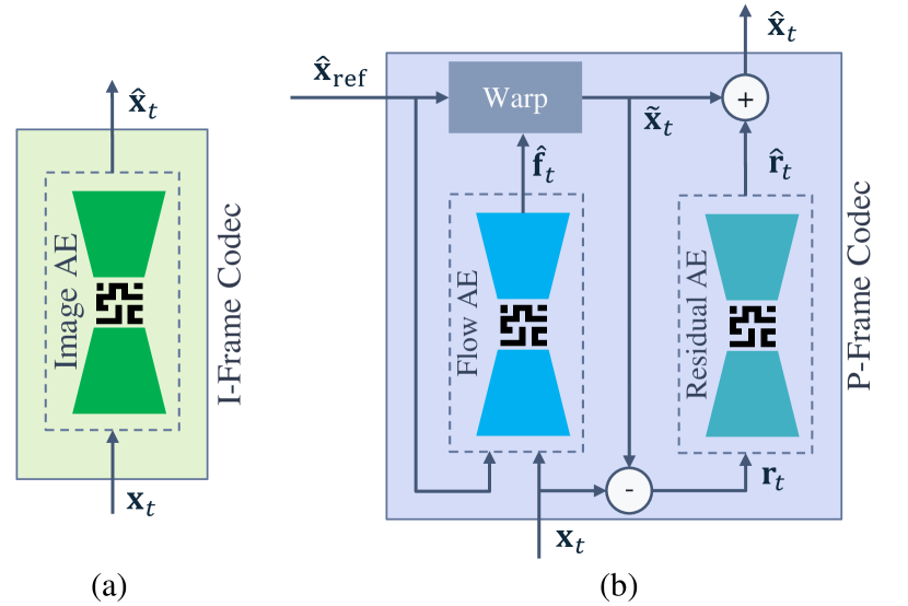
Figure 4: Block diagrams of (a) I-frame and (b) P-frame codecs, both based on $\operatorname{SSF}$ [2]. See section 3.2 for more details.

3.2 I-/P-frame codecs

Our I-frame and P-frame codecs are depicted in Fig. 4. While the I-frame codec consists of a single autoencoder $\operatorname{Image-AE}$ that compresses $\mathbf{x}_{t}$ to a reconstruction $\widehat{\mathbf{x}}_{t}$, the P-frame codec first generates a prediction $\widetilde{\mathbf{x}}_{t}$ of $\mathbf{x}_{t}$ through motion estimation via $\operatorname{Flow-AE}$ and motion compensation via $\operatorname{Warp}$ and then corrects $\widetilde{\mathbf{x}}_{t}$ using residuals via $\operatorname{Residual-AE}$ to reconstruct $\widehat{\mathbf{x}}_{t}$

$$\widehat{\mathbf{f}}_{t} =\operatorname{Flow-AE}\big{(}\mathbf{x}_{t},\>\widehat{\mathbf{x}}_{\textup{ref}}\big{)},\>\>\>\> \widetilde{\mathbf{x}}_{t} =\operatorname{Warp}\big{(}\widehat{\mathbf{x}}_{\textup{ref}},\>\widehat{\mathbf{f}}_{t}\big{)}$$

$$\mathbf{r}_{t} =\mathbf{x}_{t}-\widetilde{\mathbf{x}}_{t}, \widehat{\mathbf{r}}_{t} =\operatorname{Residual-AE}\big{(}\mathbf{r}_{t}\big{)}$$ (3)

$$\widehat{\mathbf{x}}_{t} =\widetilde{\mathbf{x}}_{t}+\widehat{\mathbf{r}}_{t}$$

where $\widehat{\mathbf{f}}_{t}$, $\mathbf{r}_{t}$, and $\widehat{\mathbf{r}}_{t}$ denote optical flow, encoder residual, and decoder residual, respectively.

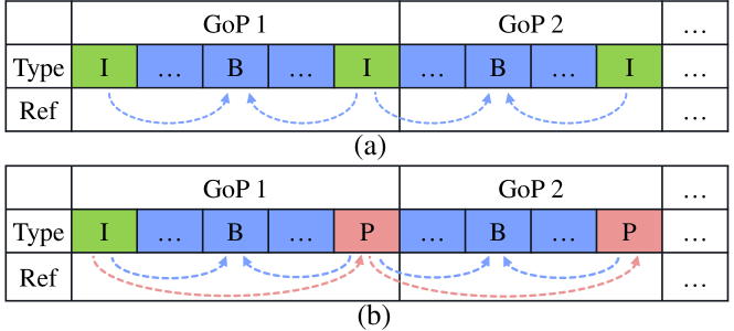
Figure 5: Frame type selection, the first reference of a video is always coded as I-frame. (a) In the $\operatorname{IBI}$ configuration, the subsequent references are coded as I-frame as well while (b) in the $\operatorname{IBP}$ configuration, they are coded as P-frame. The arrows show the references used in inter-coding.

In $\operatorname{SSF}$, $\widehat{\mathbf{f}}_{t}$ consists of spatial and scale displacement maps and $\operatorname{Warp}$ is a trilinear interpolation operator on a blur stack of $\widehat{\mathbf{x}}_{\textup{ref}}$. While $\operatorname{SSF}$ uses Gaussian filters to generate a blur stack and uses scale to non-linearly point to the blur stack, we generate the blur stack using a Gaussian pyramid followed by bilinearly upsampling all pyramid scales to the original resolution and use scale to linearly point to the blur stack.

All the above autoencoders i.e. $\operatorname{Image-AE}$, $\operatorname{Flow-AE}$, and $\operatorname{Residual-AE}$, have the same architecture (without weight sharing) based on the mean-scale hyperprior model [5] that consists of a main autoencoder (an encoder and a decoder) and a hyperprior (a hyper-encoder, a mean hyper-decoder and a scale hyper-decoder) where all the components are parameterized via convolutional neural networks. The quantized latent variables $\mathbf{z}$ are broken down into a latent and a hyper-latent where the latent has a Gaussian prior whose probabilities are conditioned on the hyper-latent and the hyper-latent has a data-independent factorized prior. See Appendix A for more details about the architecture.

3.3 GoP structure

3.3.1 Frame type selection

I-frame is the least efficient frame type in terms of coding efficiency, next is P-frame, and finally B-frame delivers the best performance. Since $\operatorname{B-EPIC}$ supports all three frame types, it is important to use the right frame type to improve the overall coding efficiency.

In neural video coding, reference frames are often inserted at GoP boundaries. A common practice is to code reference frames as intra and use them as references to code the other frames as inter. In this work, we call this configuration $\operatorname{IBI}$ where GoP boundaries are coded as I-frames and the middle frames are coded as B-frames. See Fig. 1.a for an illustration. On the other hand, given that I-frames are the least efficient among the three frame types, we can code some references as P-frames to improve the performance. Here, we call this configuration $\operatorname{IBP}$ as shown in Fig. 1.b where the first reference is coded as an I-frame and the subsequent references are coded as P-frames [33] .

3.3.2 B-frames order

Once a B-frame is coded, it can be used as a reference for the next B-frames. It is thus very important to code the B-frames in a GoP in the optimal order to i) maximally exploit the information available through the available references and ii) derive good references for the next B-frames.

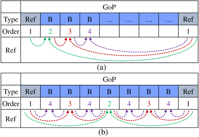
Figure 6: B-frames order, (a) $\operatorname{sequential}$, (b) $\operatorname{hierarchical}$.

Here, we present two ways to traverse the B-frames in a GoP, $\operatorname{sequential}$ and $\operatorname{hierarchical}$ [33] as shown in Fig. 6. We assume that for each given GoP, the boundary frames are references that are already available (decoded) and the middle frames are B-frames.

In the $\operatorname{sequential}$ order, we start from one end of GoP and code one B-frame at a time until we reach the other end while in the $\operatorname{hierarchical}$ order, we always code the middle frame of two references as the next B-frame. The plain $\operatorname{hierarchical}$ order only supports GoP sizes that are a power of 2 plus 1 e.g. 9, 17, 33. However, we devised an algorithm based on bisection to traverse a GoP with an arbitrary size in the $\operatorname{hierarchical}$ order as shown in Algorithm 1.

Assumption: Given a GoP of size $N$, suppose $\widehat{\mathbf{x}}_{0}$ and $\widehat{\mathbf{x}}_{N-1}$ are available as references. ;

Initialize an empty $\mathbf{stack}$ ;

push $(i_{\textup{min}},i_{\textup{max}})=(0,N-1)$ to $\mathbf{stack}$ ;

while $\mathbf{stack}$ is not empty do

       pop $\mathbf{stack}$ to retrieve $(i_{\textup{min}},i_{\textup{max}})$ ;

       Define new index $i=\operatorname{floor}((i_{\textup{min}}+i_{\textup{max}})/2)$ ;

       Encode $\mathbf{x}_{i}$ as a B-frame to generate $\widehat{\mathbf{x}}_{i}$. Use $\widehat{\mathbf{x}}_{i_{\textup{min}}}$ and $\widehat{\mathbf{x}}_{i_{\textup{max}}}$ as references ;

       if $i-i_{\textup{min}}>1$ then

             push $(i_{\textup{min}},i)$ to $\mathbf{stack}$

       end if

      if $i_{\textup{max}}-i>1$ then

             push $(i,i_{\textup{max}})$ to $\mathbf{stack}$

       end if

      

end while

Algorithm 1 Traversing an arbitrary size GoP in $\operatorname{hierarchical}$ order.

3.4 Loss function

We assume that the training is done on GoPs of $N$ frames whose boundaries are references. The loss function for the $\operatorname{IBP}$ configuration is defined as a rate-distortion tradeoff as follows:

$$\sum_{t=0}^{N-1}D\big{(}\mathbf{x}_{t},\>\widehat{\mathbf{x}}_{t}\big{)}+\beta\bigg{[}H\big{(}\textbf{z}_{0}^{i})+\sum_{t=1}^{N-1}\bigg{(}H\big{(}\textbf{z}_{t}^{f}\big{)}+H\big{(}\textbf{z}_{t}^{r}\big{)}\bigg{)}\bigg{]}$$ (4)

where $H(\cdot)$ represents the entropy estimate of a latent in terms of bits-per-pixel which corresponds to the expected size in the bitstream, $\textbf{z}_{0}^{i}$ denotes the latent of the I-frame codec’s $\operatorname{Image-AE}$, $\textbf{z}_{t}^{f}$ and $\textbf{z}_{t}^{r}$ represent the latents of the P-frame codec’s $\operatorname{Flow-AE}$ and $\operatorname{Residual-AE}$, $D(\cdot,\cdot)$ denotes distortion in terms of $\operatorname{MSE}$ or $\operatorname{MS-SSIM}$ [40], and $\beta$ is a hyperparameter that controls the balance between rate and distortion. The loss function for $\operatorname{IBI}$ is similar.

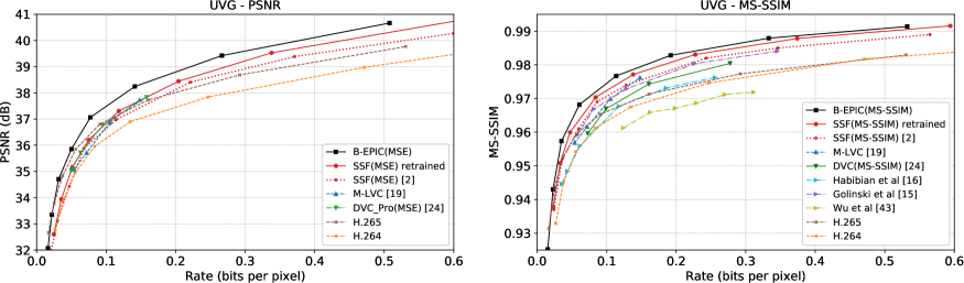
Figure 7: Rate-distortion comparison on the UVG dataset.

Figure 8: Rate-distortion comparison on the MCL-JCV dataset.

4 Experiments & Results

4.1 Training setup

Dataset: We used Vimeo-90k as training dataset [46]. It consists of $89,800$ 7-frame sequences in RGB format.

Trained models: We trained models at various rate-distortion tradeoffs ($\beta$ values), using both $\operatorname{MSE}$ and $\operatorname{MS-SSIM}$ as distortion losses. The $\operatorname{MSE}$ models $\operatorname{B-EPIC(MSE)}$ were trained on $\beta=2^{\gamma}\times 10^{-4}:\gamma\in\big{\{}0,1,...,7\big{\}}$ and the $\operatorname{MS-SSIM}$ models $\operatorname{B-EPIC(MS-SSIM)}$ were trained on $\beta=2^{\gamma}\times 10^{-2}:\gamma\in\big{\{}0,1,...,7\big{\}}$, where both $\operatorname{MSE}$ and $\operatorname{MS-SSIM}$ were measured in the RGB color space.

Training plan: we followed the exact schedule provided in $\operatorname{SSF}$ [2] to train the $\operatorname{MSE}$ and $\operatorname{MS-SSIM}$ models to facilitate comparison. Specifically, we initially trained all models for 1,000,000 gradient updates on $\operatorname{MSE}$, then trained the $\operatorname{MS-SSIM}$ models for extra 200,000 gradient updates on $\operatorname{MS-SSIM}$, and finally fine-tuned all the models for 50,000 gradient updates.

In both training and fine-tuning steps, we employed the Adam optimizer [18], used batch size of 8, and trained the network on 4-frame sequences, so the training GoP structure was IBBI and IBBP for the $\operatorname{IBI}$ and $\operatorname{IBP}$ models, respectively. The training step took about 10 days on an Nvidia V100 GPU. We tried other training GoP lengths as well. Longer GoP lengths, despite dramatically slowing down the training, did not improve the performance significantly. In the training step, we set the learning-rate to $10^{-4}$ and used randomly extracted $256\times 256$ patches. In the fine-tuning step, we reduced the learning-rate to $10^{-5}$ and increased the patch size to $256\times 384$.

We started all the components in our network from random weights except $\operatorname{FlowNet}$ in the interpolation block where a pretrained $\operatorname{PWC-Net}$ with frozen weights was employed. The gradient from B-frame codecs was stopped from propagating to the I-frame and P-frame codecs for more stable training [2].

4.2 Evaluation setup

We evaluated $\operatorname{B-EPIC}$ on the UVG [38], MCL-JCV [39], and HEVC [7] datasets, all of which are widely used in the neural video codec literature. All these datasets are available in YUV420. We used FFMPEG [14] to convert the videos to RGB that is acceptable by $\operatorname{B-EPIC}$ (and almost all other neural codecs). See Appendix B for the FFMPEG commands details.

As shown in section 4.5, the $\operatorname{hierarchical}$ B-frame order together with the $\operatorname{IBP}$ GoP structure generate our best results. The results we report in the rest of this section are based on these settings as well as an evaluation GoP size of 12 for consistency with other works [24, 43].

We report video quality in terms of $\operatorname{PSNR}$ and $\operatorname{MS-SSIM}$ where both are first calculated per-frame in the RGB color space, then averaged over all the frames of each video, and finally averaged over all the videos of a dataset. Due to the network architecture, our codec accepts inputs whose spatial dimensions are a multiple of 64. Whenever there is a size incompatibility, we pad the frame to the nearest multiple of 64 before feeding to the encoder, and crop the decoded frame to compensate for padding. This issue, which may be fixable, could lead to a coding inefficiency depending on the number of pixels that have to be padded.

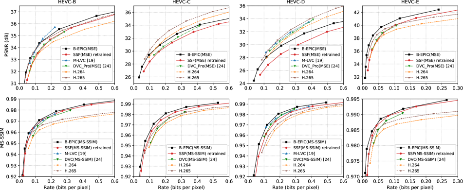
Figure 9: Rate-distortion comparison on the HEVC dataset.

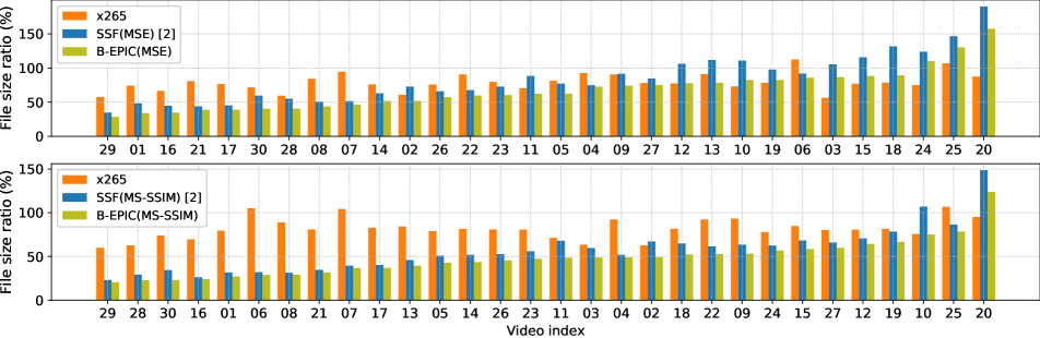
Figure 10: File sizes generated by $\operatorname{H.265}$, $\operatorname{SSF}$, and $\operatorname{B-EPIC}$ relative to $\operatorname{H.264}$ on the MCL-JCV dataset, measured by $\operatorname{PSNR}$ (top) and $\operatorname{MS-SSIM}$ (bottom) BD-rate gain. A value of 100% translates to equal sizes and no bit-rate savings. Smaller values are preferable.

4.3 Compared methods

We compared our results with several neural video codecs including $\operatorname{SSF}$ [2], DVC [24], M-LVC [19], Golinski et al.  [15], Wu et al.  [43], and Habibian et al.  [16]. We reimplemented and trained $\operatorname{SSF}$, and here provide both the original results reported in the paper as well as the reproduced results. The results in the original paper where obtained with GoP size of infinity i.e. only the first frame of a sequence is an I-frame and the rest are all P-frames while we report the performance on GoP of 12.

The standard codecs that we compare with are $\operatorname{H.264}$ [41] and $\operatorname{H.265}$ [34]. We generated the results for both using FFMPEG where GoP size of 12 was used with all the other default settings. This is unlike the other papers that limit the FFMPEG performance by not allowing B-frames, or changing the preset to fast or superfast. See Appendix B for the FFMPEG commands details.

4.4 Results & Discussion

Rate-distortion: the rate-distortion comparisons on the UVG, MCL-JCV, and HEVC datasets are shown in Figs. 7, 8, 9, respectively.

When evaluated in terms of $\operatorname{MS-SSIM}$, $\operatorname{B-EPIC(MS-SSIM)}$ outperforms all the compared methods on all the datasets across all bit-rates.

When evaluated in terms of $\operatorname{PSNR}$, as can be observed from Figs. 7 and 8, $\operatorname{B-EPIC(MSE)}$ significantly outperforms all the competing neural codecs as well as $\operatorname{H.264}$ across all bit-rates on both UVG and MCL-JCV datasets. Compared to $\operatorname{H.265}$, $\operatorname{B-EPIC(MSE)}$ maintains a large margin in the average and high bit-rates and is roughly on-par in extremely low bit-rate cases. On the HEVC dataset, the results are similarly favorable on HEVC class-B and class-E. On class-C, the standard codecs outperform all neural methods, and on class-D $\operatorname{B-EPIC(MSE)}$ performs poorly. This is most likely due to the fact that the class-D videos have to be padded from $240\times 416$ to the nearest multiple of $64$, i.e. $256\times 448$, before it can be fed to our encoder. This means our method in its current form has to encode $15\%$ more pixels, all of which are discarded on the decoder side. It is worth noting that HEVC class-D is already removed in the common test conditions of the most recent standard video codec $\operatorname{H.266}$ [8] due to very small resolution.

$\operatorname{B-EPIC}$ can be thought of as a B-frame equivalent of $\operatorname{SSF}$ and as can be observed from the rate-distortion comparisons, outperforms $\operatorname{SSF}$ significantly across all bit-rates on all the datasets. This proves the effectiveness of our B-frame approach when applied to an existing P-frame codec.

Bjøntegaard delta rate (BD-rate): in this section, we report BD-rate [6] gains versus $\operatorname{H.264}$. Table 1 lists the average BD-rate gains versus $\operatorname{H.264}$ on the UVG, MCL-JCV, and HEVC datasets in terms of both $\operatorname{PSNR}$ and $\operatorname{MS-SSIM}$. Here, the numbers show how much a method can save on bit-rate compared to $\operatorname{H.264}$ while generating the same video quality. $\operatorname{B-EPIC}$ yields the highest $\operatorname{MS-SSIM}$ BD-rate gains and performs relatively well in terms of $\operatorname{PSNR}$ BD-rate gains.

	$\operatorname{PSNR}$ BD-rate gain (%)			$\operatorname{MS-SSIM}$ BD-rate gain (%)
Dataset	$\operatorname{H.265}$	$\operatorname{SSF}$	$\operatorname{B-EPIC}$	$\operatorname{H.265}$	$\operatorname{SSF}$	$\operatorname{B-EPIC}$
		$\operatorname{(MSE)}$	$\operatorname{(MSE)}$		$\operatorname{(MS-SSIM)}$	$\operatorname{(MS-SSIM)}$
UVG	-28.66	-25.71	-47.89	-24.03	-41.05	-50.79
MCL-JCV	-20.86	-15.90	-31.91	-18.22	-43.25	-52.12
HEVC-B	-25.0	-16.28	-35.68	-19.70	-48.23	-55.19
HEVC-C	-19.51	47.69	11.22	-15.80	-27.32	-41.53
HEVC-D	-16.25	82.89	29.05	-11.86	-20.79	-43.98
HEVC-E	-32.53	-24.35	-53.87	-30.45	-47.81	-61.32
HEVC-Avg	-23.32	22.49	-12.32	-19.46	-36.04	-50.50

Table 1: Average BD-rate gain versus $\operatorname{H.264}$ on different datasets.

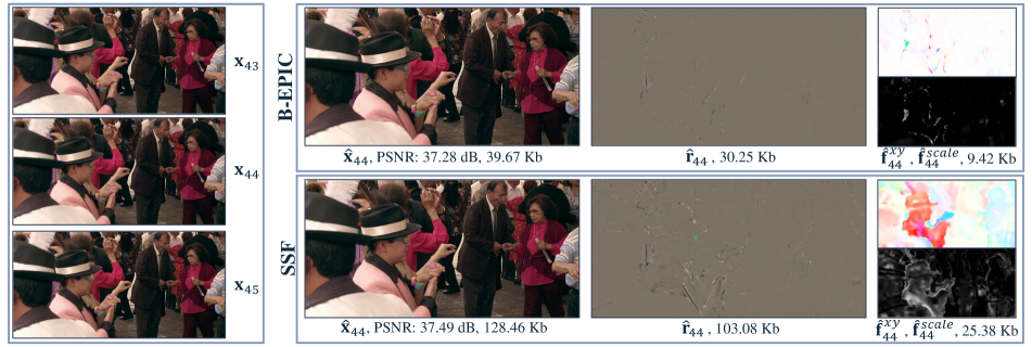
Figure 11: Qualitative results on frame 44 of Tango video from Netflix Tango in Netflix El Fuente [44]. $\mathbf{x}_{43}$, $\mathbf{x}_{44}$, and $\mathbf{x}_{45}$ are an input sequence. In $\operatorname{SSF}$, $\mathbf{x}_{44}$ is coded as a P-frame with $\mathbf{\widehat{x}}_{43}$ used as reference. In $\operatorname{B-EPIC}$, $\mathbf{x}_{44}$ is coded as a B-frame with both $\mathbf{\widehat{x}}_{43}$ and $\mathbf{\widehat{x}}_{45}$ used as references. The interpolation block delivers an accurate baseline frame used in the P-frame codec as reference. As a result, both flow and residual are less detailed and consume fewer bits compared to $\operatorname{SSF}$.

Furthermore, in Fig 10 we show the file sizes of the individual MCL-JCV videos encoded using $\operatorname{B-EPIC}$, $\operatorname{SSF}$, and $\operatorname{H.265}$ compared to $\operatorname{H.264}$, estimated by BD-rate. As observed here, $\operatorname{B-EPIC}$ delivers better results compared to $\operatorname{SSF}$ across the board. Compared to $\operatorname{H.265}$, it performs significantly better on the majority of the videos, specially in terms of $\operatorname{MS-SSIM}$. The under-performance on the last sequences of the figure is potentially because they are animated movies, while our training dataset Vimeo-90k is only comprised of natural videos, as pointed out in [2] as well.

Qualitative results: Fig. 2 shows a sample qualitative result where an input sequence together with the decoded frames, optical flow maps, and residuals for $\operatorname{SSF}$ and $\operatorname{B-EPIC}$ are visualized. $\operatorname{B-EPIC}$ relies on much less detailed optical flow and residuals due to the frame-interpolation outcome being used as reference, and as a result, generates a lot less bits compared to $\operatorname{SSF}$ at a similar $\operatorname{PSNR}$.

Per-frame performance: Fig. 12 shows how $\operatorname{B-EPIC}$ performs on average across a GoP of 12 frames when using the $\operatorname{sequential}$ and $\operatorname{hierarchical}$ B-frames orders on the UVG dataset. As expected, as the gap between the two references closes (by newly coded B-frames used as reference), $\operatorname{PSNR}$ improves and Rate drops.

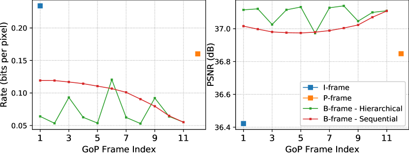
Figure 12: Average per-frame results across a GoP of 12 for the $\operatorname{sequential}$ and $\operatorname{hierarchical}$ B-frames orders on the UVG dataset. The first frame of each sequence is coded I, the last frame of each GoP is coded P, and the rest are coded B.

4.5 Ablation studies

We studied the effectiveness of different components of our codec including: GoP structure ($\operatorname{IBI}$ vs $\operatorname{IBP}$), B-frames order ($\operatorname{sequential}$ vs $\operatorname{hierarchical}$), pretraining $\operatorname{PWC-Net}$, and removing $\operatorname{Flow-AE}$ for the P-frame codec and relying only on $\operatorname{Residual-AE}$. The last configuration where $\operatorname{Flow-AE}$ is removed, is similar to the B-frame codecs that use interpolation followed by residual correction [11]. These ablation studies are shown in Fig. 13.a. Moreover, we studied the effect of the training GoP on the performance by finetuning our model on different sequences including: 4 consecutive frames, 7 consecutive frames, and 4 frames where consecutive frames are two frames apart. All the studied configurations delivered similar rate-distortion results on the UVG datasets. So, we proceeded with 4 consecutive frames as it is the most memory efficient and fastest to train.

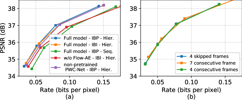
Figure 13: Ablations studies on the UVG dataset, (a) effectiveness of each component, (b) effect of the training sequence length/shape on the performance.

5 Conclusion

In this paper, we proposed a method to add B-frame coding capability to an existing neural P-frame codec by adding an interpolation block. It significantly improves the performance of the P-frame codec and delivers state-of-the-art neural video coding results on multiple datasets. Since the prototype we developed in this work is based on 2-reference B-frames and 1-reference P-frame codecs, as a future direction, this idea can be extended to the cases where more that 2 references are available to B-frames and/or with multi-frame P-frame codecs

Appendix

Appendix A Architecture details

A.1 I-/P-frame codec

The details of the main autoencoder and the hyperprior in $\operatorname{Image-AE}$, $\operatorname{Flow-AE}$, and $\operatorname{Residual-AE}$ are shown in Figs. 14 and 15, respectively.

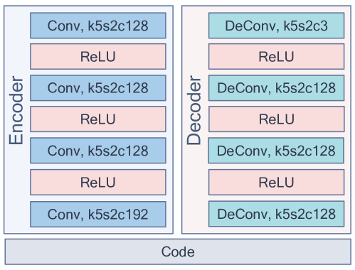
Figure 14: Main autoencoder details. $k$, $s$, and $c$ denote kernel size, stride, and the number of output channels, respectively.

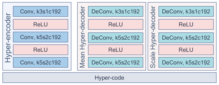
Figure 15: Hyperprior details. $k$, $s$, and $c$ denote kernel size, stride, and the number of output channels, respectively.

In our implementation of the hyperprior, we followed [5] which differs slightly from $\operatorname{SSF}$ [2] as pointed below:

• in the scale hyper-decoder, $\operatorname{QReLU}$ activations are replaced by $\operatorname{ReLU}$ and the last $\operatorname{QReLU}$ is removed. To have a lower bound on standard deviation values, we clamp the scale hyper-decoder output at $0.11$,

• in both hyper-decoders, the last layer is implemented as a $\operatorname{DeConv}\>3\times 3$ with stride 1 as opposed to $\operatorname{DeConv}\>5\times 5$ with stride 2 in $\operatorname{SSF}$,

• the hyper-encoder, the first layer is implemented as a $\operatorname{Conv}\>3\times 3$ with stride 1 as opposed to $\operatorname{Conv}\>5\times 5$ with stride 2 in $\operatorname{SSF}$.

A.2 Frame interpolation

In the frame interpolation component, $\operatorname{FlowNet}$ is a pre-trained $\operatorname{PWC-Net}$ [35] without modifications and $\operatorname{RefineNet}$ is a $\operatorname{U-Net}$ shown in Fig. 16.

Figure 16: U-Net architecture details. $k$, $s$, and $c$ denote kernel size, stride, and the number of output channels, respectively.

Appendix B FFMPEG commands

We generated $\operatorname{H.264}$ and $\operatorname{H.265}$ baselines using FFMPEG. The command that we used to run FFMPEG with all the default configurations is as follows:

ffmpeg -pix_fmt yuv420p -s [W]x[H] -r [FR] -i [IN].yuv -c:v libx[ENC] -b:v -crf [CRF] [OUT].mkv

and the command that we used to run FFMPEG with GoP=12 is as follows:

ffmpeg -pix_fmt yuv420p -s [W]x[H] -r [FR] -i [IN].yuv -c:v libx[ENC] -b:v -crf [CRF] -x[ENC]-params "keyint=[GOP]:min-keyint=[GOP]:verbose=1" [OUT].mkv

where the values in brackets represent the encoder parameters as follows: H and W are the frame dimensions, FR is the frame rate, ENC is the encoder type (x264 or x265), GOP is the GoP size (12), INPUT and OUTPUT are the input and the output filenames, respectively, and CRF controls the bit-rate (We tried CRF$=\{9,12,15,18,21,24,27,30\}$).

In order to measure $\operatorname{MS-SSIM}$ and $\operatorname{PSNR}$ in the RGB color space, we saved all video frames as PNG files using FFMPEG using the following commands for YUV and MKV files:

ffmpeg -pix_fmt yuv420p -s [W]x[H] -i [IN].yuv %9d.png

ffmpeg [IN].mkv %9d.png

Appendix C Extended results

Bjøntegaard delta rate (BD-rate) comparison: We report the BD-rate [6] gains for a scenario where both $\operatorname{H.264}$ and $\operatorname{H.265}$ are configured to use all the default parameters as opposed to the results for GoP=12 reported in 4.4 (see Table 2).

	$\operatorname{PSNR}$ BD-rate gain (%)			$\operatorname{MS-SSIM}$ BD-rate gain (%)
Dataset	$\operatorname{H.265}$	$\operatorname{SSF}$	$\operatorname{B-EPIC}$	$\operatorname{H.265}$	$\operatorname{SSF}$	$\operatorname{B-EPIC}$
		$\operatorname{(MSE)}$	$\operatorname{(MSE)}$		$\operatorname{(MS-SSIM)}$	$\operatorname{(MS-SSIM)}$
UVG	-29.02	11.05	-26.93	-24.28	-11.55	-25.99
MCL-JCV	-20.06	3.77	-17.27	-16.76	-29.69	-40.76
HEVC-B	-22.44	6.69	-18.21	-16.54	-32.36	-41.80
HEVC-C	-12.96	91.98	43.38	-8.21	-5.24	-24.66
HEVC-D	-7.64	149.80	72.16	-3.13	5.71	-27.71
HEVC-E	-27.31	34.28	-18.12	-27.24	-4.36	-30.77
HEVC-Avg	-17.59	70.69	19.80	-13.78	-9.05	-31.23

Table 2: Average BD-rate gain versus $\operatorname{H.264}$ (with FFMPEG default parameters) on different datasets.

Qualitative results:

In Fig. 17 we show the intermediate visualizations as well as the detailed rate-distortion results across a GoP of seven frames for both $\operatorname{B-EPIC}$ and $\operatorname{SSF}$. Figures 18 and 19 show qualitative comparisons of $\operatorname{B-EPIC}$ and $\operatorname{SSF}$ for the first GoP of two videos.

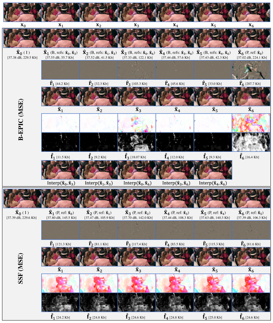
Figure 17: Qualitative results for the first GoP (GoP=7) of Tango video from Netflix Tango in Netflix El Fuente [44] (resolution $1024\times 2048$, zoom in for more details). Both $\operatorname{B-EPIC}$ and $\operatorname{SSF}$ models are trained on $\operatorname{MSE}$ with $\beta=0.0016$. $\mathbf{x}_{0}$ is an intra frame with similar performance on $\operatorname{B-EPIC}$ and $\operatorname{SSF}$. The other six frames are inter frames (P or B). $\operatorname{SSF}$ yields consistent bit-rates across the inter frames due to similar level of details in the optical flow and the residuals. That is mainly because all the inter frames are P-frames where the immediate previous decoded frame is used as reference. In $\operatorname{B-EPIC}$, the inter frames are mostly B-frames where the distances to the references are quite variable. As a result, it delivers different bit-rates across the inter frames. The average results for the inter-frames for $\operatorname{B-EPIC}$ and $\operatorname{SSF}$ are as follows: $\operatorname{PSNR}$: 37.37dB vs 37.57dB, bit-rate: 90.5 Kb vs 124.7 kb, residual bit-rate: 77.7 Kb vs 100.0 Kb, flow bit-rate: 12.8 Kb vs 24.7 Kb. Here, the bit-rate values are obtained by multiplying $\operatorname{Rate}$ (bits-per-pixel) by frame resolution.
[Video produced by Netflix, with CC BY-NC-ND 4.0 license: https://media.xiph.org/video/derf/ElFuente/Netflix_Tango_Copyright.txt]

Figure 18: Qualitative comparisons of $\operatorname{B-EPIC}$ and $\operatorname{SSF}$. The columns represent a sequence of 7 frames (top to bottom) compressed using $\operatorname{B-EPIC}$ and $\operatorname{SSF}$ as well as the uncompressed sequence where the GoP structures for $\operatorname{B-EPIC}$ and $\operatorname{SSF}$ are IBBBBBP and IPPPPPP, respectively. The average (size, $\operatorname{PSNR}$) for $\operatorname{B-EPIC}$ and $\operatorname{SSF}$ are (43.47KB, 28.80dB) and (51.39KB, 28.85dB). While $\operatorname{B-EPIC}$ generates similar $\operatorname{PSNR}$ and visual quality, it consumes 15.4% less bits compared to $\operatorname{SSF}$. [Video obtained from Pexels.]

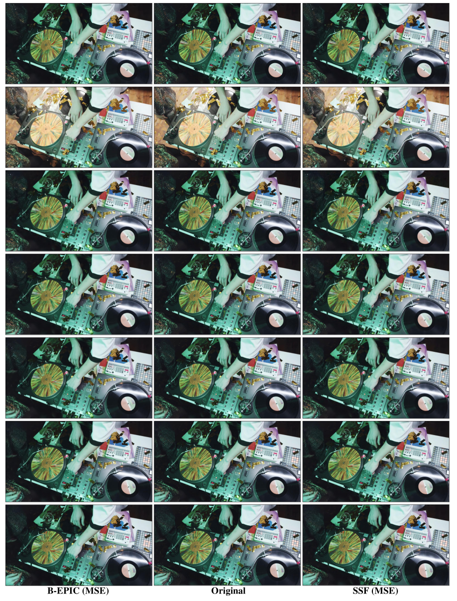
Figure 19: Qualitative comparisons of $\operatorname{B-EPIC}$ and $\operatorname{SSF}$. The columns represent a sequence of 7 frames (top to bottom) compressed using $\operatorname{B-EPIC}$ and $\operatorname{SSF}$ as well as the uncompressed sequence where the GoP structures for $\operatorname{B-EPIC}$ and $\operatorname{SSF}$ are IBBBBBP and IPPPPPP, respectively. The average (size, $\operatorname{PSNR}$) for $\operatorname{B-EPIC}$ and $\operatorname{SSF}$ are (23.84KB, 33.81dB) and (27.01KB, 33.94dB). While $\operatorname{B-EPIC}$ generates similar $\operatorname{PSNR}$ and visual quality, it consumes 11.7% less bits compared to $\operatorname{SSF}$. [Video obtained from Pexels.]

Rate-distortion results: We report the per-video performance of our $\operatorname{B-EPIC(MSE)}$ and $\operatorname{B-EPIC(MS-SSIM)}$ models on the UVG [38], MCL-JCV [39], and HEVC [7] datasets in Tables 3 through 14.

	Performance across models - $\operatorname{PSNR}$ (dB) vs $\operatorname{Rate}$ (bits-per-pixel)
Video	$\operatorname{Rate}$	$\operatorname{PSNR}$	$\operatorname{Rate}$	$\operatorname{PSNR}$	$\operatorname{Rate}$	$\operatorname{PSNR}$	$\operatorname{Rate}$	$\operatorname{PSNR}$	$\operatorname{Rate}$	$\operatorname{PSNR}$	$\operatorname{Rate}$	$\operatorname{PSNR}$	$\operatorname{Rate}$	$\operatorname{PSNR}$	$\operatorname{Rate}$	$\operatorname{PSNR}$
Beauty	0.956	37.92	0.553	36.8	0.229	35.53	0.061	34.51	0.029	34.16	0.018	33.9	0.012	33.54	0.009	33.1
Bosphorus	0.235	42.71	0.12	41.41	0.067	40.09	0.04	38.8	0.025	37.34	0.016	36.0	0.013	34.45	0.01	33.1
HoneyBee	0.415	39.87	0.112	38.56	0.036	37.66	0.017	36.68	0.01	35.49	0.007	34.4	0.007	33.01	0.006	31.68
Jockey	0.419	40.79	0.193	39.73	0.11	39.0	0.071	38.29	0.053	37.42	0.034	36.59	0.026	35.44	0.02	34.18
ReadySetGo	0.455	41.38	0.28	40.14	0.178	38.75	0.119	37.26	0.084	35.65	0.054	34.12	0.039	32.46	0.031	30.77
ShakeNDry	0.599	40.13	0.292	38.7	0.159	37.42	0.094	36.17	0.058	34.81	0.035	33.46	0.02	31.92	0.013	30.68
YachtRide	0.474	41.87	0.316	40.64	0.21	39.28	0.139	37.75	0.091	36.1	0.057	34.46	0.036	32.6	0.024	30.96
Average	0.508	40.67	0.267	39.43	0.141	38.25	0.077	37.07	0.05	35.85	0.032	34.71	0.022	33.35	0.016	32.07

Table 3: Detailed rate-distortion performance of $\operatorname{B-EPIC(MSE)}$ on the UVG dataset.

	Performance across models - $\operatorname{MS-SSIM}$ vs $\operatorname{Rate}$ (bits-per-pixel)
Video	$\operatorname{Rate}$	$\operatorname{MS-SSIM}$	$\operatorname{Rate}$	$\operatorname{MS-SSIM}$	$\operatorname{Rate}$	$\operatorname{MS-SSIM}$	$\operatorname{Rate}$	$\operatorname{MS-SSIM}$	$\operatorname{Rate}$	$\operatorname{MS-SSIM}$	$\operatorname{Rate}$	$\operatorname{MS-SSIM}$	$\operatorname{Rate}$	$\operatorname{MS-SSIM}$	$\operatorname{Rate}$	$\operatorname{MS-SSIM}$
Beauty	0.842	0.98	0.607	0.973	0.377	0.961	0.21	0.946	0.102	0.928	0.031	0.906	0.017	0.898	0.01	0.892
Bosphorus	0.37	0.995	0.203	0.993	0.112	0.99	0.065	0.986	0.035	0.98	0.021	0.972	0.015	0.959	0.012	0.942
HoneyBee	0.47	0.992	0.253	0.989	0.105	0.985	0.054	0.981	0.01	0.974	0.016	0.966	0.011	0.95	0.008	0.934
Jockey	0.589	0.991	0.365	0.987	0.207	0.981	0.115	0.976	0.07	0.969	0.039	0.962	0.03	0.952	0.02	0.934
ReadySetGo	0.413	0.995	0.245	0.993	0.146	0.99	0.095	0.986	0.063	0.98	0.039	0.971	0.028	0.958	0.02	0.939
ShakeNDry	0.573	0.992	0.362	0.988	0.207	0.983	0.135	0.976	0.065	0.966	0.049	0.954	0.027	0.929	0.018	0.905
YachtRide	0.47	0.995	0.296	0.993	0.19	0.99	0.121	0.986	0.08	0.98	0.05	0.971	0.03	0.954	0.019	0.931
Average	0.532	0.991	0.333	0.988	0.192	0.983	0.114	0.977	0.061	0.968	0.035	0.957	0.023	0.943	0.015	0.925

Table 4: Detailed rate-distortion performance of $\operatorname{B-EPIC(MS-SSIM)}$ on the UVG dataset.

	Performance across models - $\operatorname{PSNR}$ (dB) vs $\operatorname{Rate}$ (bits-per-pixel)
Video	$\operatorname{Rate}$	$\operatorname{PSNR}$	$\operatorname{Rate}$	$\operatorname{PSNR}$	$\operatorname{Rate}$	$\operatorname{PSNR}$	$\operatorname{Rate}$	$\operatorname{PSNR}$	$\operatorname{Rate}$	$\operatorname{PSNR}$	$\operatorname{Rate}$	$\operatorname{PSNR}$	$\operatorname{Rate}$	$\operatorname{PSNR}$	$\operatorname{Rate}$	$\operatorname{PSNR}$
videoSRC01	0.371	40.88	0.093	39.54	0.036	38.96	0.017	38.49	0.011	37.97	0.007	37.39	0.007	36.65	0.006	35.88
videoSRC02	0.19	44.26	0.124	43.36	0.086	42.36	0.061	41.23	0.046	39.94	0.032	38.64	0.025	37.09	0.02	35.36
videoSRC03	0.328	41.5	0.166	40.29	0.09	39.08	0.05	37.78	0.029	36.31	0.018	35.07	0.013	33.62	0.01	32.07
videoSRC04	0.858	41.28	0.648	39.92	0.481	38.46	0.339	36.71	0.231	35.07	0.152	33.55	0.093	31.88	0.056	30.36
videoSRC05	0.905	37.94	0.467	36.77	0.266	35.89	0.169	35.0	0.113	34.01	0.074	33.0	0.051	31.68	0.038	30.25
videoSRC06	1.374	33.86	1.021	33.42	0.647	32.51	0.169	31.15	0.016	30.63	0.009	30.54	0.007	30.43	0.006	30.3
videoSRC07	0.895	37.22	0.55	36.31	0.253	35.18	0.111	34.33	0.061	33.64	0.038	32.99	0.025	32.16	0.017	31.37
videoSRC08	0.62	38.96	0.205	37.69	0.1	37.1	0.054	36.5	0.031	35.8	0.019	35.03	0.014	34.14	0.011	33.2
videoSRC09	1.107	38.1	0.744	36.83	0.446	35.4	0.233	33.74	0.128	32.05	0.078	30.42	0.05	28.59	0.035	26.83
videoSRC10	0.899	40.18	0.612	38.8	0.417	37.32	0.286	35.81	0.202	34.29	0.132	32.77	0.093	31.08	0.084	29.35
videoSRC11	0.274	44.58	0.186	43.39	0.126	42.07	0.086	40.65	0.061	39.1	0.039	37.58	0.028	36.0	0.022	34.33
videoSRC12	0.338	41.55	0.19	39.79	0.11	38.04	0.061	36.18	0.034	34.47	0.02	32.94	0.014	31.55	0.011	30.18
videoSRC13	0.781	39.28	0.544	38.11	0.347	36.65	0.176	34.74	0.067	32.58	0.024	30.35	0.012	27.8	0.009	25.8
videoSRC14	0.544	40.75	0.284	39.46	0.166	38.37	0.107	37.26	0.072	36.05	0.048	34.8	0.035	33.38	0.026	31.89
videoSRC15	1.0	38.48	0.63	37.19	0.329	35.69	0.139	33.99	0.054	32.41	0.03	31.18	0.02	29.87	0.014	28.55
videoSRC16	0.232	41.51	0.09	40.68	0.05	40.14	0.03	39.49	0.02	38.75	0.013	37.94	0.011	36.98	0.008	35.81
videoSRC17	0.525	40.34	0.244	39.15	0.152	38.29	0.097	37.36	0.065	36.28	0.043	35.12	0.029	33.73	0.021	32.49
videoSRC18	0.316	39.3	0.191	37.82	0.12	36.89	0.079	35.19	0.055	33.49	0.034	31.83	0.024	29.98	0.017	28.45
videoSRC19	0.517	41.81	0.333	40.35	0.219	38.82	0.145	37.24	0.096	35.61	0.061	34.05	0.041	32.51	0.03	31.07
videoSRC20	0.409	42.06	0.284	40.84	0.202	39.6	0.14	38.08	0.1	36.57	0.068	35.13	0.05	33.66	0.038	32.13
videoSRC21	0.172	45.04	0.111	44.25	0.075	43.46	0.052	42.54	0.036	41.5	0.025	40.38	0.019	39.1	0.015	37.78
videoSRC22	0.525	42.84	0.348	41.5	0.242	40.23	0.172	38.91	0.124	37.49	0.088	35.95	0.063	34.29	0.046	32.58
videoSRC23	0.317	43.45	0.186	42.05	0.113	40.61	0.072	39.13	0.047	37.57	0.031	36.04	0.022	34.47	0.016	32.88
videoSRC24	0.333	41.48	0.216	40.51	0.146	39.68	0.095	38.53	0.061	37.07	0.039	35.76	0.027	33.95	0.02	32.22
videoSRC25	1.084	36.19	0.809	35.27	0.594	34.45	0.411	33.06	0.27	31.49	0.174	30.02	0.107	28.09	0.067	26.31
videoSRC26	0.243	42.55	0.138	41.65	0.093	40.85	0.065	39.94	0.047	38.89	0.034	37.8	0.026	36.48	0.021	34.9
videoSRC27	0.447	42.4	0.299	40.89	0.2	39.28	0.132	37.59	0.086	35.82	0.054	34.12	0.034	32.3	0.023	30.7
videoSRC28	0.178	42.72	0.085	41.74	0.046	40.74	0.027	39.63	0.018	38.44	0.012	37.16	0.011	35.8	0.009	34.39
videoSRC29	0.071	45.3	0.035	44.59	0.021	43.96	0.013	43.28	0.009	42.5	0.007	41.71	0.006	40.84	0.005	39.79
videoSRC30	0.286	40.02	0.144	39.26	0.054	38.36	0.022	37.52	0.013	36.72	0.009	35.94	0.008	35.06	0.007	34.08
Average	0.538	40.86	0.333	39.71	0.208	38.62	0.12	37.37	0.073	36.08	0.047	34.84	0.032	33.44	0.024	32.04

Table 5: Detailed rate-distortion performance of $\operatorname{B-EPIC(MSE)}$ on the MCL-JCV dataset.

	Performance across models - $\operatorname{MS-SSIM}$ vs $\operatorname{Rate}$ (bits-per-pixel)
Video	$\operatorname{Rate}$	$\operatorname{MS-SSIM}$	$\operatorname{Rate}$	$\operatorname{MS-SSIM}$	$\operatorname{Rate}$	$\operatorname{MS-SSIM}$	$\operatorname{Rate}$	$\operatorname{MS-SSIM}$	$\operatorname{Rate}$	$\operatorname{MS-SSIM}$	$\operatorname{Rate}$	$\operatorname{MS-SSIM}$	$\operatorname{Rate}$	$\operatorname{MS-SSIM}$	$\operatorname{Rate}$	$\operatorname{MS-SSIM}$
videoSRC01	0.567	0.991	0.347	0.987	0.178	0.982	0.078	0.976	0.021	0.97	0.009	0.966	0.008	0.961	0.006	0.955
videoSRC02	0.312	0.996	0.177	0.995	0.106	0.993	0.068	0.99	0.047	0.987	0.031	0.982	0.025	0.976	0.018	0.964
videoSRC03	0.467	0.994	0.273	0.992	0.136	0.988	0.064	0.983	0.029	0.976	0.016	0.968	0.014	0.957	0.011	0.941
videoSRC04	0.634	0.994	0.45	0.991	0.318	0.986	0.223	0.98	0.154	0.971	0.1	0.957	0.065	0.935	0.04	0.907
videoSRC05	0.642	0.988	0.415	0.984	0.249	0.979	0.144	0.972	0.085	0.963	0.051	0.952	0.035	0.933	0.023	0.9
videoSRC06	0.9	0.95	0.652	0.938	0.433	0.919	0.269	0.896	0.108	0.865	0.016	0.839	0.009	0.834	0.004	0.83
videoSRC07	0.756	0.981	0.512	0.975	0.307	0.966	0.158	0.955	0.08	0.944	0.043	0.932	0.029	0.917	0.019	0.902
videoSRC08	0.708	0.986	0.487	0.982	0.272	0.975	0.117	0.967	0.041	0.96	0.018	0.953	0.013	0.946	0.009	0.934
videoSRC09	0.62	0.994	0.371	0.991	0.211	0.985	0.125	0.978	0.067	0.966	0.041	0.948	0.029	0.922	0.021	0.887
videoSRC10	0.58	0.995	0.388	0.993	0.263	0.99	0.171	0.985	0.114	0.979	0.071	0.971	0.05	0.96	0.038	0.945
videoSRC11	0.29	0.996	0.175	0.995	0.114	0.993	0.077	0.991	0.054	0.987	0.034	0.982	0.026	0.975	0.018	0.963
videoSRC12	0.259	0.995	0.146	0.992	0.086	0.988	0.066	0.983	0.032	0.973	0.019	0.961	0.014	0.945	0.011	0.926
videoSRC13	0.338	0.995	0.158	0.991	0.072	0.986	0.036	0.979	0.011	0.971	0.006	0.959	0.006	0.941	0.007	0.923
videoSRC14	0.526	0.994	0.326	0.991	0.191	0.987	0.111	0.983	0.067	0.976	0.041	0.968	0.03	0.956	0.021	0.938
videoSRC15	0.727	0.992	0.501	0.988	0.315	0.982	0.174	0.972	0.075	0.956	0.039	0.939	0.018	0.911	0.013	0.883
videoSRC16	0.461	0.992	0.264	0.988	0.127	0.984	0.055	0.98	0.026	0.976	0.015	0.971	0.012	0.965	0.008	0.949
videoSRC17	0.604	0.992	0.385	0.989	0.227	0.985	0.133	0.979	0.078	0.972	0.051	0.963	0.034	0.949	0.022	0.929
videoSRC18	0.215	0.994	0.136	0.991	0.089	0.986	0.066	0.98	0.041	0.969	0.026	0.954	0.02	0.932	0.015	0.897
videoSRC19	0.496	0.995	0.326	0.993	0.213	0.989	0.139	0.984	0.089	0.976	0.055	0.965	0.037	0.947	0.025	0.925
videoSRC20	0.326	0.996	0.228	0.994	0.16	0.991	0.116	0.987	0.079	0.98	0.053	0.97	0.04	0.956	0.029	0.931
videoSRC21	0.261	0.995	0.146	0.992	0.085	0.99	0.053	0.988	0.036	0.985	0.024	0.981	0.019	0.976	0.013	0.968
videoSRC22	0.48	0.995	0.323	0.993	0.216	0.99	0.148	0.986	0.106	0.981	0.074	0.974	0.055	0.962	0.038	0.944
videoSRC23	0.334	0.996	0.196	0.995	0.113	0.992	0.068	0.989	0.04	0.984	0.027	0.978	0.019	0.968	0.014	0.954
videoSRC24	0.303	0.996	0.182	0.995	0.112	0.992	0.071	0.99	0.045	0.986	0.028	0.98	0.02	0.969	0.014	0.946
videoSRC25	0.637	0.994	0.447	0.991	0.302	0.987	0.207	0.98	0.135	0.968	0.085	0.951	0.054	0.923	0.033	0.874
videoSRC26	0.388	0.994	0.216	0.991	0.115	0.988	0.069	0.985	0.045	0.981	0.031	0.977	0.024	0.969	0.018	0.956
videoSRC27	0.374	0.996	0.238	0.994	0.158	0.992	0.107	0.988	0.066	0.982	0.043	0.973	0.027	0.957	0.018	0.937
videoSRC28	0.272	0.994	0.128	0.992	0.055	0.99	0.027	0.988	0.015	0.985	0.01	0.981	0.008	0.975	0.007	0.965
videoSRC29	0.19	0.995	0.089	0.993	0.042	0.991	0.02	0.989	0.012	0.987	0.007	0.984	0.007	0.98	0.006	0.975
videoSRC30	0.294	0.989	0.138	0.985	0.048	0.981	0.021	0.976	0.009	0.971	0.006	0.965	0.007	0.957	0.006	0.946
Average	0.465	0.992	0.294	0.989	0.177	0.984	0.106	0.979	0.06	0.971	0.036	0.961	0.025	0.949	0.017	0.93

Table 6: Detailed rate-distortion performance of $\operatorname{B-EPIC(MS-SSIM)}$ on the MCL-JCV dataset.

	Performance across models - $\operatorname{PSNR}$ (dB) vs $\operatorname{Rate}$ (bits-per-pixel)
Video	$\operatorname{Rate}$	$\operatorname{PSNR}$	$\operatorname{Rate}$	$\operatorname{PSNR}$	$\operatorname{Rate}$	$\operatorname{PSNR}$	$\operatorname{Rate}$	$\operatorname{PSNR}$	$\operatorname{Rate}$	$\operatorname{PSNR}$	$\operatorname{Rate}$	$\operatorname{PSNR}$	$\operatorname{Rate}$	$\operatorname{PSNR}$	$\operatorname{Rate}$	$\operatorname{PSNR}$
BQTerrace	1.18	36.28	0.799	35.4	0.414	34.13	0.185	32.9	0.089	31.61	0.046	30.32	0.026	28.75	0.018	27.15
BasketballDrive	0.858	37.98	0.411	36.76	0.219	35.85	0.13	34.93	0.083	33.93	0.053	32.91	0.036	31.55	0.026	30.15
Cactus	0.986	36.74	0.525	35.69	0.239	34.64	0.108	33.51	0.06	32.39	0.036	31.27	0.023	29.89	0.017	28.58
Kimono	0.55	39.96	0.247	38.69	0.138	37.7	0.082	36.67	0.052	35.49	0.034	34.32	0.023	32.97	0.017	31.75
ParkScene	0.805	38.02	0.445	36.73	0.241	35.39	0.122	33.83	0.061	32.2	0.034	30.78	0.021	29.33	0.016	28.11
Average	0.876	37.8	0.486	36.66	0.25	35.54	0.125	34.37	0.069	33.13	0.041	31.92	0.026	30.5	0.019	29.15

Table 7: Detailed rate-distortion performance of $\operatorname{B-EPIC(MSE)}$ on the HEVC class-B dataset.

	Performance across models - $\operatorname{MS-SSIM}$ vs $\operatorname{Rate}$ (bits-per-pixel)
Video	$\operatorname{Rate}$	$\operatorname{MS-SSIM}$	$\operatorname{Rate}$	$\operatorname{MS-SSIM}$	$\operatorname{Rate}$	$\operatorname{MS-SSIM}$	$\operatorname{Rate}$	$\operatorname{MS-SSIM}$	$\operatorname{Rate}$	$\operatorname{MS-SSIM}$	$\operatorname{Rate}$	$\operatorname{MS-SSIM}$	$\operatorname{Rate}$	$\operatorname{MS-SSIM}$	$\operatorname{Rate}$	$\operatorname{MS-SSIM}$
BQTerrace	0.635	0.987	0.413	0.983	0.238	0.977	0.12	0.968	0.049	0.956	0.026	0.94	0.014	0.911	0.01	0.881
BasketballDrive	0.608	0.989	0.381	0.985	0.22	0.98	0.121	0.974	0.065	0.964	0.038	0.952	0.026	0.933	0.017	0.896
Cactus	0.7	0.987	0.452	0.982	0.243	0.975	0.122	0.965	0.048	0.952	0.028	0.939	0.018	0.917	0.013	0.893
Kimono	0.587	0.992	0.371	0.988	0.211	0.983	0.119	0.977	0.063	0.968	0.04	0.958	0.026	0.941	0.017	0.92
ParkScene	0.628	0.991	0.416	0.986	0.244	0.98	0.139	0.971	0.064	0.956	0.036	0.936	0.018	0.904	0.013	0.872
average	0.632	0.989	0.407	0.985	0.231	0.979	0.124	0.971	0.058	0.959	0.033	0.945	0.02	0.921	0.014	0.892

Table 8: Detailed rate-distortion performance of $\operatorname{B-EPIC(MS-SSIM)}$ on the HEVC class-B dataset.

	Performance across models - $\operatorname{PSNR}$ (dB) vs $\operatorname{Rate}$ (bits-per-pixel)
Video	$\operatorname{Rate}$	$\operatorname{PSNR}$	$\operatorname{Rate}$	$\operatorname{PSNR}$	$\operatorname{Rate}$	$\operatorname{PSNR}$	$\operatorname{Rate}$	$\operatorname{PSNR}$	$\operatorname{Rate}$	$\operatorname{PSNR}$	$\operatorname{Rate}$	$\operatorname{PSNR}$	$\operatorname{Rate}$	$\operatorname{PSNR}$	$\operatorname{Rate}$	$\operatorname{PSNR}$
BQMall	0.741	38.11	0.436	36.97	0.269	35.83	0.168	34.33	0.105	32.65	0.063	31.06	0.04	29.24	0.027	27.43
BaskehallDrill	0.68	36.6	0.392	35.48	0.257	34.4	0.167	33.06	0.106	31.63	0.066	30.35	0.042	28.69	0.029	27.01
PartyScene	1.182	33.32	0.799	32.6	0.546	31.72	0.354	30.27	0.202	28.38	0.107	26.61	0.054	24.58	0.031	22.91
RaceHorses	1.175	36.33	0.834	35.44	0.589	34.43	0.395	32.96	0.249	31.27	0.145	29.7	0.076	27.86	0.046	26.37
Average	0.945	36.09	0.615	35.12	0.415	34.09	0.271	32.65	0.165	30.98	0.095	29.43	0.053	27.59	0.033	25.93

Table 9: Detailed rate-distortion performance of $\operatorname{B-EPIC(MSE)}$ on the HEVC class-C dataset.

	Performance across models - $\operatorname{MS-SSIM}$ vs $\operatorname{Rate}$ (bits-per-pixel)
Video	$\operatorname{Rate}$	$\operatorname{MS-SSIM}$	$\operatorname{Rate}$	$\operatorname{MS-SSIM}$	$\operatorname{Rate}$	$\operatorname{MS-SSIM}$	$\operatorname{Rate}$	$\operatorname{MS-SSIM}$	$\operatorname{Rate}$	$\operatorname{MS-SSIM}$	$\operatorname{Rate}$	$\operatorname{MS-SSIM}$	$\operatorname{Rate}$	$\operatorname{MS-SSIM}$	$\operatorname{Rate}$	$\operatorname{MS-SSIM}$
BQMall	0.439	0.993	0.235	0.989	0.13	0.985	0.077	0.978	0.045	0.968	0.025	0.953	0.018	0.932	0.014	0.902
BasketballDrill	0.451	0.991	0.275	0.987	0.162	0.98	0.096	0.968	0.055	0.951	0.033	0.928	0.025	0.899	0.017	0.853
PartyScene	0.474	0.99	0.288	0.986	0.165	0.979	0.098	0.965	0.053	0.942	0.03	0.904	0.021	0.855	0.014	0.796
RaceHorses	0.758	0.991	0.524	0.987	0.35	0.981	0.231	0.973	0.138	0.957	0.075	0.932	0.041	0.893	0.025	0.843
average	0.531	0.991	0.33	0.987	0.202	0.981	0.125	0.971	0.073	0.954	0.041	0.93	0.026	0.895	0.017	0.849

Table 10: Detailed rate-distortion performance of $\operatorname{B-EPIC(MS-SSIM)}$ on the HEVC class-C dataset.

	Performance across models - $\operatorname{PSNR}$ (dB) vs $\operatorname{Rate}$ (bits-per-pixel)
Video	$\operatorname{Rate}$	$\operatorname{PSNR}$	$\operatorname{Rate}$	$\operatorname{PSNR}$	$\operatorname{Rate}$	$\operatorname{PSNR}$	$\operatorname{Rate}$	$\operatorname{PSNR}$	$\operatorname{Rate}$	$\operatorname{PSNR}$	$\operatorname{Rate}$	$\operatorname{PSNR}$	$\operatorname{Rate}$	$\operatorname{PSNR}$	$\operatorname{Rate}$	$\operatorname{PSNR}$
BQSquare	1.249	34.09	0.87	33.36	0.593	32.21	0.391	30.58	0.217	28.49	0.109	26.59	0.043	24.38	0.02	22.24
BasketballPass	0.883	36.99	0.623	35.85	0.449	34.74	0.308	33.21	0.197	31.45	0.121	29.88	0.072	28.1	0.047	26.44
BlowingBubbles	1.124	33.82	0.729	32.92	0.468	31.96	0.281	30.46	0.154	28.63	0.08	26.95	0.042	25.07	0.025	23.47
RaceHorses	1.253	36.63	0.903	35.55	0.648	34.3	0.434	32.68	0.268	30.81	0.154	29.07	0.083	27.19	0.053	25.61
Average	1.127	35.38	0.781	34.42	0.539	33.31	0.354	31.73	0.209	29.85	0.116	28.12	0.06	26.19	0.036	24.44

Table 11: Detailed rate-distortion performance of $\operatorname{B-EPIC(MSE)}$ on the HEVC class-D dataset.

	Performance across models - $\operatorname{MS-SSIM}$ vs $\operatorname{Rate}$ (bits-per-pixel)
Video	$\operatorname{Rate}$	$\operatorname{MS-SSIM}$	$\operatorname{Rate}$	$\operatorname{MS-SSIM}$	$\operatorname{Rate}$	$\operatorname{MS-SSIM}$	$\operatorname{Rate}$	$\operatorname{MS-SSIM}$	$\operatorname{Rate}$	$\operatorname{MS-SSIM}$	$\operatorname{Rate}$	$\operatorname{MS-SSIM}$	$\operatorname{Rate}$	$\operatorname{MS-SSIM}$	$\operatorname{Rate}$	$\operatorname{MS-SSIM}$
BQSquare	0.4	0.991	0.228	0.987	0.121	0.981	0.066	0.972	0.029	0.952	0.011	0.921	0.008	0.889	0.008	0.851
BasketballPass	0.477	0.993	0.311	0.99	0.208	0.984	0.137	0.975	0.084	0.961	0.05	0.939	0.033	0.908	0.021	0.857
BlowingBubbles	0.393	0.989	0.22	0.984	0.117	0.975	0.066	0.96	0.035	0.936	0.019	0.897	0.015	0.851	0.01	0.797
RaceHorses	0.697	0.992	0.474	0.989	0.317	0.983	0.206	0.973	0.125	0.956	0.064	0.928	0.037	0.892	0.022	0.835
average	0.492	0.992	0.308	0.987	0.191	0.981	0.119	0.97	0.068	0.951	0.036	0.921	0.023	0.885	0.015	0.835

Table 12: Detailed rate-distortion performance of $\operatorname{B-EPIC(MS-SSIM)}$ on the HEVC class-D dataset.

	Performance across models - $\operatorname{PSNR}$ (dB) vs $\operatorname{Rate}$ (bits-per-pixel)
Video	$\operatorname{Rate}$	$\operatorname{PSNR}$	$\operatorname{Rate}$	$\operatorname{PSNR}$	$\operatorname{Rate}$	$\operatorname{PSNR}$	$\operatorname{Rate}$	$\operatorname{PSNR}$	$\operatorname{Rate}$	$\operatorname{PSNR}$	$\operatorname{Rate}$	$\operatorname{PSNR}$	$\operatorname{Rate}$	$\operatorname{PSNR}$	$\operatorname{Rate}$	$\operatorname{PSNR}$
Vidyo1	0.234	42.17	0.108	40.84	0.052	39.65	0.029	38.44	0.018	37.06	0.012	35.68	0.01	33.95	0.008	32.24
Vidyo3	0.243	42.48	0.125	41.17	0.066	39.81	0.037	38.46	0.022	36.78	0.014	35.08	0.011	33.1	0.009	31.24
Vidyo4	0.241	42.61	0.118	41.17	0.058	39.73	0.032	38.36	0.019	36.85	0.012	35.39	0.01	33.68	0.008	32.12
Average	0.239	42.42	0.117	41.06	0.059	39.73	0.033	38.42	0.02	36.89	0.013	35.39	0.01	33.58	0.009	31.87

Table 13: Detailed rate-distortion performance of $\operatorname{B-EPIC(MSE)}$ on the HEVC class-E dataset.

	Performance across models - $\operatorname{MS-SSIM}$ vs $\operatorname{Rate}$ (bits-per-pixel)
Video	$\operatorname{Rate}$	$\operatorname{MS-SSIM}$	$\operatorname{Rate}$	$\operatorname{MS-SSIM}$	$\operatorname{Rate}$	$\operatorname{MS-SSIM}$	$\operatorname{Rate}$	$\operatorname{MS-SSIM}$	$\operatorname{Rate}$	$\operatorname{MS-SSIM}$	$\operatorname{Rate}$	$\operatorname{MS-SSIM}$	$\operatorname{Rate}$	$\operatorname{MS-SSIM}$	$\operatorname{Rate}$	$\operatorname{MS-SSIM}$
Vidyo1	0.298	0.994	0.154	0.992	0.07	0.988	0.032	0.984	0.013	0.979	0.008	0.972	0.009	0.962	0.008	0.95
Vidyo3	0.254	0.995	0.112	0.992	0.047	0.989	0.026	0.985	0.012	0.979	0.008	0.97	0.009	0.956	0.008	0.941
Vidyo4	0.243	0.995	0.118	0.992	0.054	0.989	0.031	0.985	0.014	0.979	0.009	0.972	0.009	0.959	0.008	0.947
average	0.265	0.995	0.128	0.992	0.057	0.989	0.029	0.985	0.013	0.979	0.009	0.971	0.009	0.959	0.008	0.946

Table 14: Detailed rate-distortion performance of $\operatorname{B-EPIC(MS-SSIM)}$ on the HEVC class-E dataset.

References

- [1] Eirikur Agustsson, Fabian Mentzer, Michael Tschannen, Lukas Cavigelli, Radu Timofte, Luca Benini, and Luc V Gool. Soft-to-hard vector quantization for end-to-end learning compressible representations. In Advances in Neural Information Processing Systems, volume 30. Curran Associates, Inc., 2017.
- [2] Eirikur Agustsson, David Minnen, Nick Johnston, Johannes Balle, Sung Jin Hwang, and George Toderici. Scale-space flow for end-to-end optimized video compression. In Proceedings of the IEEE/CVF Conference on Computer Vision and Pattern Recognition (CVPR), June 2020.
- [3] Johannes Ballé, Valero Laparra, and Eero P. Simoncelli. Density modeling of images using a generalized normalization transformation. Jan. 2016. 4th International Conference on Learning Representations, ICLR 2016.
- [4] J. Ballé, V. Laparra, and E. P. Simoncelli. End-to-end optimization of nonlinear transform codes for perceptual quality. In 2016 Picture Coding Symposium (PCS), pages 1–5, 2016.
- [5] Johannes Ballé, David Minnen, Saurabh Singh, Sung Jin Hwang, and Nick Johnston. Variational image compression with a scale hyperprior. In International Conference on Learning Representations, 2018.
- [6] Gisle Bjøntegaard. Calculation of average PSNR differences between RD-curves. Doc. VCEG-M33. ITU-T SG16/Q6 VCEG, Austin, TX, USA, July 2001.
- [7] Frank Bossen. Common test conditions and software reference configurations. JCTVC-F900, 2011.
- [8] B. Bross, J. Chen, S. Liu, and Y.-K. Wang. Versatile video coding (draft 10). Output document JVET-S2001, July 2020.
- [9] Meixu Chen, Todd Goodall, Anjul Patney, and Alan C. Bovik. Learning to compress videos without computing motion, 2020.
- [10] T. Chen, H. Liu, Z. Ma, Q. Shen, X. Cao, and Y. Wang. End-to-end learnt image compression via non-local attention optimization and improved context modeling. IEEE Transactions on Image Processing, 30:3179–3191, 2021.
- [11] Zhengxue Cheng, Heming Sun, Masaru Takeuchi, and Jiro Katto. Learning image and video compression through spatial-temporal energy compaction. In Proceedings of the IEEE/CVF Conference on Computer Vision and Pattern Recognition (CVPR), June 2019.
- [12] Yoojin Choi, Mostafa El-Khamy, and Jungwon Lee. Variable rate deep image compression with a conditional autoencoder. In Proceedings of the IEEE/CVF International Conference on Computer Vision (ICCV), October 2019.
- [13] Abdelaziz Djelouah, Joaquim Campos, Simone Schaub-Meyer, and Christopher Schroers. Neural inter-frame compression for video coding. In Proceedings of the IEEE/CVF International Conference on Computer Vision (ICCV), October 2019.
- [14] ffmpeg Developers. ffmpeg. http://ffmpeg.org/. Accessed: 2020-02-21.
- [15] Adam Golinski, Reza Pourreza, Yang Yang, Guillaume Sautiere, and Taco S. Cohen. Feedback recurrent autoencoder for video compression. In Proceedings of the Asian Conference on Computer Vision (ACCV), November 2020.
- [16] Amirhossein Habibian, Ties van Rozendaal, Jakub M. Tomczak, and Taco S. Cohen. Video compression with rate-distortion autoencoders. In Proceedings of the IEEE/CVF International Conference on Computer Vision (ICCV), October 2019.
- [17] Huaizu Jiang, Deqing Sun, Varun Jampani, Ming-Hsuan Yang, Erik Learned-Miller, and Jan Kautz. Super slomo: High quality estimation of multiple intermediate frames for video interpolation. In Proceedings of the IEEE Conference on Computer Vision and Pattern Recognition (CVPR), June 2018.
- [18] Diederik P. Kingma and Jimmy Ba. Adam: A method for stochastic optimization, 2015. International Conference for Learning Representations, San Diego, 2015.
- [19] Jianping Lin, Dong Liu, Houqiang Li, and Feng Wu. M-LVC: Multiple frames prediction for learned video compression. In Proceedings of the IEEE/CVF Conference on Computer Vision and Pattern Recognition (CVPR), June 2020.
- [20] H. Liu, M. Lu, Z. Ma, F. Wang, Z. Xie, X. Cao, and Y. Wang. Neural video coding using multiscale motion compensation and spatiotemporal context model. IEEE Transactions on Circuits and Systems for Video Technology, pages 1–1, 2020.
- [21] Haojie Liu, Han Shen, Lichao Huang, Ming Lu, Tong Chen, and Zhan Ma. Learned video compression via joint spatial-temporal correlation exploration. Proceedings of the AAAI Conference on Artificial Intelligence, 34(07):11580–11587, Apr. 2020.
- [22] Salvator Lombardo, Jun Han, Christopher Schroers, and Stephan Mandt. Deep generative video compression. In Advances in Neural Information Processing Systems, volume 32. Curran Associates, Inc., 2019.
- [23] Guo Lu, Wanli Ouyang, Dong Xu, Xiaoyun Zhang, Chunlei Cai, and Zhiyong Gao. DVC: An end-to-end deep video compression framework. In Proceedings of the IEEE/CVF Conference on Computer Vision and Pattern Recognition (CVPR), June 2019.
- [24] G. Lu, X. Zhang, W. Ouyang, L. Chen, Z. Gao, and D. Xu. An end-to-end learning framework for video compression. IEEE Transactions on Pattern Analysis and Machine Intelligence, 2020.
- [25] Yadong Lu, Yinhao Zhu, Yang Yang, Amir Said, and Taco S Cohen. Progressive neural image compression with nested quantization and latent ordering, 2021.
- [26] Fabian Mentzer, Eirikur Agustsson, Michael Tschannen, Radu Timofte, and Luc Van Gool. Conditional probability models for deep image compression. In Proceedings of the IEEE Conference on Computer Vision and Pattern Recognition (CVPR), June 2018.
- [27] David Minnen, Johannes Ballé, and George D Toderici. Joint autoregressive and hierarchical priors for learned image compression. In S. Bengio, H. Wallach, H. Larochelle, K. Grauman, N. Cesa-Bianchi, and R. Garnett, editors, Advances in Neural Information Processing Systems, volume 31. Curran Associates, Inc., 2018.
- [28] David Minnen and Saurabh Singh. Channel-wise autoregressive entropy models for learned image compression. In IEEE International Conference on Image Processing (ICIP), 2020.
- [29] W. Park and M. Kim. Deep predictive video compression using mode-selective uni- and bi-directional predictions based on multi-frame hypothesis. IEEE Access, 9:72–85, 2021.
- [30] Oren Rippel and Lubomir Bourdev. Real-time adaptive image compression. In Proceedings of the 34th International Conference on Machine Learning, volume 70, pages 2922–2930, 06–11 Aug 2017.
- [31] Oren Rippel, Sanjay Nair, Carissa Lew, Steve Branson, Alexander G. Anderson, and Lubomir Bourdev. Learned video compression. In Proceedings of the IEEE/CVF International Conference on Computer Vision (ICCV), October 2019.
- [32] Olaf Ronneberger, Philipp Fischer, and Thomas Brox. U-net: Convolutional networks for biomedical image segmentation. In Medical Image Computing and Computer-Assisted Intervention – MICCAI 2015, pages 234–241, Cham, 2015. Springer International Publishing.
- [33] H. Schwarz, D. Marpe, and T. Wiegand. Analysis of hierarchical b pictures and mctf. In 2006 IEEE International Conference on Multimedia and Expo, pages 1929–1932, 2006.
- [34] G J Sullivan, J R Ohm, W J Han, and T Wiegand. Overview of the High Efficiency Video Coding (HEVC) Standard. IEEE Trans. Circuits Syst. Video Technol., 22(12):1649–1668, Dec. 2012.
- [35] D. Sun, X. Yang, M. Liu, and J. Kautz. PWC-Net: Cnns for optical flow using pyramid, warping, and cost volume. In 2018 IEEE/CVF Conference on Computer Vision and Pattern Recognition, pages 8934–8943, 2018.
- [36] George Toderici, Sean M. O’Malley, Sung Jin Hwang, Damien Vincent, David Minnen, Shumeet Baluja, Michele Covell, and Rahul Sukthankar. Variable rate image compression with recurrent neural networks. CoRR, abs/1511.06085, 2015.
- [37] George Toderici, Damien Vincent, Nick Johnston, Sung Jin Hwang, David Minnen, Joel Shor, and Michele Covell. Full resolution image compression with recurrent neural networks. In Proceedings of the IEEE Conference on Computer Vision and Pattern Recognition (CVPR), July 2017.
- [38] Ultra Video Group. UVG test sequences. http://ultravideo.cs.tut.fi/. Accessed: 2020-02-21.
- [39] H. Wang, W. Gan, S. Hu, J. Y. Lin, L. Jin, L. Song, P. Wang, I. Katsavounidis, A. Aaron, and C. . J. Kuo. Mcl-jcv: A jnd-based h.264/avc video quality assessment dataset. In 2016 IEEE International Conference on Image Processing (ICIP), pages 1509–1513, 2016.
- [40] Zhou Wang, Alan C Bovik, Hamid R Sheikh, Eero P Simoncelli, et al. Image quality assessment: from error visibility to structural similarity. IEEE Trans. on Image Processing, 13(4):600–612, 2004.
- [41] T. Wiegand, G. J. Sullivan, G. Bjontegaard, and A. Luthra. Overview of the H.264/AVC video coding standard. IEEE Transactions on Circuits and Systems for Video Technology, 13(7):560–576, July 2003.
- [42] Mathias Wien. High Efficiency Video Coding: Coding Tools and Specification. Springer Publishing Company, Incorporated, 2014.
- [43] Chao-Yuan Wu, Nayan Singhal, and Philipp Krahenbuhl. Video compression through image interpolation. In Proceedings of the European Conference on Computer Vision (ECCV), September 2018.
- [44] Xiph.org. Xiph.org video test media [derf’s collection]. https://media.xiph.org/video/derf/. Accessed: 2020-02-21.
- [45] Xiangyu Xu, Li Siyao, Wenxiu Sun, Qian Yin, and Ming-Hsuan Yang. Quadratic video interpolation. In Advances in Neural Information Processing Systems, volume 32. Curran Associates, Inc., 2019.
- [46] Tianfan Xue, Baian Chen, Jiajun Wu, Donglai Wei, and William T Freeman. Video enhancement with task-oriented flow. International Journal of Computer Vision (IJCV), 127(8):1106–1125, 2019.
- [47] Ruihan Yang, Yibo Yang, Joseph Marino, and Stephan Mandt. Hierarchical autoregressive modeling for neural video compression. In International Conference on Learning Representations, 2021.