Ion acceleration to MeV by the ExB wave mechanism in collisionless shocks

Abstract

It is shown that ions can be accelerated to MeV energy range in the direction perpendicular to the magnetic field by the ExB mechanism of electrostatic waves. The acceleration occurs in discrete steps of duration being a small fraction the gyroperiod and can explain observations of ion energization to 10 keV at quasi-perpendicular shocks and to 100-1000 keV at quasi-parallel shocks. A general expression is provided for the maximum energy of ions accelerated in shocks of arbitrary configuration. The waves involved in the acceleration are related to three cross-field current-driven instabilities: the lower hybrid drift (LHD) instability induced by the density gradients in shocks and shocklets, followed by the modified two-stream (MTS) and electron cyclotron drift (ECD) instabilities, induced by the ExB drift of electrons in the strong LHD wave electric field. The ExB wave mechanism accelerates heavy ions to energies proportional to the atomic mass number, which is consistent with satellite observations upstream of the bow shock and also with observations of post-shocks in supernovae remnants.

1 Introduction

When the solar wind plasma streaming with a speed of 400 km s^-1 and containing protons with kinetic energy of 1 keV and the thermal spread of 20 eV interacts with the Earth’s quasi-perpendicular bow shock, the ion temperature increases by a factor of 10 across the shock, while the plasma flow slows down during the compression of the solar wind plasma and magnetic field. The heating process is also associated with the appearance of energetic particles at energies 10 keV, which implies significant acceleration of a suprathermal population of the solar wind ions. The electron temperature also undergoes a rapid increase by a factor of 10 across the shock.

On the other hand, when the interplanetary magnetic field is in the quasi-parallel direction to the shock normal, an extended upstream foreshock region (Greenstadt et al., 1995; Eastwood et al., 2005) is formed, containing ULF waves, turbulence, non-linear structures and field-aligned beams. In addition to the electron and ion heating comparable to that occurring in quasi-perpendicular shocks, observations upstream of the quasi-parallel shocks show energetic ions accelerated to hundreds keV, indicating a three to four orders of magnitude increase of the kinetic energy.

The energetic ions observed in quasi-parallel shocks are traditionally believed to be energized in a diffusive shock acceleration process. The key assumptions of this model are: (i) the solar wind ions are preheated at the shock and partially reflected upstream, (ii) there are moving barriers in the upstream region that reflect these particles back to the bow shock. After multiple bouncing between these barriers the particles gain energy through the Fermi acceleration mechanism (Fermi, 1949; Bell, 1978; Lee & Fisk, 1982; Burgess et al., 2012; Otsuka et al., 2018). Because the interplanetary shocks that could provide the upstream reflecting boundary are rare phenomena there has been a continuous search for other obstacles, such as for example foreshock transients, needed for the Fermi process to work at the bow shock. In a new attempt, Turner et al. (2018) have suggested that hot flow anomalies (Thomsen et al., 1988; Liu et al., 2016) observed occasionally in the solar wind could make such upstream barriers, or traps where the energization occurs autogenously.

All mechanisms relying on the Fermi process require nonlocal magnetic traps/mirrors, which are difficult to justify for energetic particles observed on every satellite passage upstream of the quasi-parallel shock, viz., whenever the interplanetary magnetic field changes direction to quasi-parallel. Furthermore, the foreshock transients propagate in the upstream direction, against the solar wind, so they would contribute to the deceleration and not to the acceleration of the trapped particles. Any acceleration relying on multiple bouncing would also require interaction times much longer than those implied by the observations. Thus, a local process that does not require moving magnetic mirrors, or electrostatic field barriers, would be more suitable to explain ion acceleration at quasi-parallel shocks.

It has been recently shown (Stasiewicz, 2020; Stasiewicz & Eliasson, 2020a, b) that particle heating and acceleration in collisionless shocks of arbitrary orientation are related to the wave electric fields of drift instabilities triggered by shock compression of the plasma. It is a local process that can be summarized as follows:

Shock compressions of the density N and the magnetic field B $\rightarrow$ diamagnetic current $\rightarrow$ lower hybrid drift (LHD) instability $\rightarrow$ electron E$\times$B drift $\rightarrow$ modified two-stream (MTS) and electron cyclotron drift (ECD) instabilities $\rightarrow$ heating: quasi-adiabatic ($\chi_{j}<1$), stochastic ($\chi_{j}>1$), acceleration ($\chi_{j}\gg 1$).

The stochastic heating and acceleration of particle species with charge $q_{j}$ and mass $m_{j}$ ($j=e$ for electrons, $p$ for protons, $i$ for general ions) is controlled by the function

$$\chi_{j}(t,\mathbf{r})=\frac{m_{j}}{q_{j}B^{2}}{\rm div}(\mathbf{E}_{\perp})$$ (1)

that depends on the $m/q$ ratio and is also a measure of the charge non-neutrality. It is a generalization of the heating condition from earlier works of Karney (1979); McChesney et al. (1987); Balikhin et al. (1993); Vranjes & Poedts (2010), where the divergence is reduced to the directional gradient $\partial E_{x}/\partial x$. The particles are magnetized (adiabatic) for $|\chi_{j}|<1$, demagnetized (subject to non-adiabatic heating) for $|\chi_{j}|\gtrsim 1$, and selectively accelerated to high perpendicular velocities when $|\chi_{j}|\gg 1$.

The term ’stochastic’ is here used in the sense of chaos theory for deterministic systems and does not involve random variables. At a certain threshold value of $|\chi_{j}|$, particles with initially nearby states can have positive Lyapunov exponents and divergent trajectories. This happens for $|\chi_{j}|\gtrsim 1$ when the interacting waves have zero frequencies such as at shocks or low frequencies comparable to or below the cyclotron frequency, $f\lesssim f_{cj}$ (McChesney et al., 1987; Balikhin et al., 1993; Stasiewicz et al., 2000). At higher wave frequencies $f\gg f_{cj}$ (Karney, 1979), stochastic motion sets in for particles having velocities near the phase velocity, $v\gtrsim v_{ph}=\omega/k$ with a threshold value $E/B\gtrsim(f_{cj}/f)^{1/3}v_{ph}/4$ for stochastic motion, which can be written in dimensionless variables as $|\chi_{j}|\gtrsim\Omega^{2/3}/4$ with $\Omega=f/f_{cj}$ and $|\chi_{j}|=m_{j}kE/q_{j}B^{2}$. Wave frequencies near cyclotron harmonics (Fukuyama et al., 1977) can also lead to resonant acceleration of particles with $v\gtrsim v_{ph}$ to form high-velocity tails in the distribution function. Thus, at high frequencies we have the formation of an ’acceleration lane’ indicated by a green line in Figure 1.

Previous simulations have shown that ions at perpendicular bow shocks are stochastically bulk heated with typical values of $\chi_{p}\sim 60$ produced by the electric fields of the lower hybrid drift instability. Electrons can also be heated stochastically on electron cyclotron drift waves. However, in most cases they undergo a quasi-adiabatic heating process, $T_{e\parallel}\approx T_{e\perp}\propto B^{\alpha}$, where $\alpha=1/3-2/3$ (Stasiewicz & Eliasson, 2020a, b).

The aim of this paper is to show that ions can be accelerated to MeV energies by electrostatic waves in the frequency range from the proton gyrofrequency $f_{cp}$ to the multiples of the electron gyrofrequency $nf_{ce}$ associated with the three cross-field, current-driven LHD, MTS, and ECD instabilities mentioned above. The acceleration mechanism requires $\chi\gg 1$ and can increase velocity of some particles by the E$\times$B drift velocity due to the wave electric field, i.e., by the speed $\widetilde{V}_{E}=\widetilde{E}_{\perp}/B$ (Sugihara & Midzuno, 1979; Dawson et al., 1983; Ohsawa, 1985). The E$\times$B wave mechanism is related to the surfatron mechanism at shocks (Sagdeev, 1966; Katsouleas & Dawson, 1983; Zank et al., 1996; Ucer & Shapiro, 2001; Shapiro & Ucer, 2003), which requires wide front of coherent waves and acceleration is done after multiple ion reflections between the shock and the upstream region (Zank et al., 1996; Shapiro et al., 2001). In contradistinction, the E$\times$B mechanism works on much shorter time-scales at a fraction of a cyclotron period and much shorter spatial scales to reach significant energies by the interaction with incoherent bursts of waves. It is coupled to the stochastic condition (1), which makes it possible to obtain significant acceleration of protons, $10\,\mathrm{eV}\rightarrow 200\,\mathrm{keV}$ on intermittent and bursty waves observed at shocks and in the magnetosheath.

2 Stochastic heating and acceleration

Stochastic heating and acceleration of charged particles by electrostatic waves can be studied with the simulation setup used by Stasiewicz & Eliasson (2020a, b). In the magnetic field $\mathbf{B}_{0}=(0,0,B_{0})$ there is a macroscopic convection electric field $E_{y0}$ that drives particles into an electrostatic wave $\widetilde{E}_{x}=E_{x0}\sin(\omega_{D}t-k_{x}x)$ with wavenumber $k_{x}=2\pi/\lambda$, and the Doppler shifted frequency $\omega_{D}$ in the spacecraft frame. Trajectories and velocities of particles with mass $m$ and charge $q$ are determined by the Lorentz equation $md\mathbf{v}/dt=q(\mathbf{E}+\mathbf{v}\times\mathbf{B}_{0})$. By using dimensionless variables with time normalized by $\omega_{c}^{-1}$, space by $k_{x}^{-1}$ and velocity by $\omega_{c}/k_{x}$ with $\omega_{c}=qB_{0}/m$ being the angular cyclotron frequency, a system of equations is obtained in the plasma reference frame

$$\frac{du_{x}}{dt} =\mbox{$\widetilde{\chi}\;$}\sin(\Omega t-x)+u_{y},$$ (2)

$$\frac{du_{y}}{dt} =-u_{x},$$ (3)

$$\frac{dx}{dt} =u_{x},\qquad\frac{dy}{dt}=u_{y},$$ (4)

that depends on two parameters: the normalized wave frequency in the plasma frame $\Omega=(\omega_{D}-k_{x}E_{y0}/B_{0})/\omega_{c}$, and

$$\mbox{$\widetilde{\chi}\;$}=\frac{E_{x0}}{B_{0}}\frac{k_{x}}{\omega_{c}},$$ (5)

the stochastic heating parameter (1) for a single wave mode. This is in fact the normalized amplitude of the wave induced E$\times$B drift speed $\widetilde{V}_{E,y}=\widetilde{E}_{x}/B_{0}$, not to be confused with the convection drift $V_{E,x}=-E_{y0}/B_{0}$ that is absorbed in the normalized frequency $\Omega$. The initial gyration velocity of a particle is $(v_{x0},v_{y0},0)$, and $v_{\perp 0}=(v_{x0}^{2}+v_{y0}^{2})^{1/2}$. In normalized variables it becomes

$$u_{\perp 0}=k_{\perp}v_{\perp 0}/\omega_{c}=k_{\perp}r_{c}$$ (6)

with the initial Larmor radius $r_{c}=v_{\perp{0}}/\omega_{c}$, and $k_{\perp}=k_{x}$.

For a statistical description of the particles we follow the procedure outlined in previous works (Stasiewicz & Eliasson, 2020a, b), and carry out a set of test particle simulations for $M=1,000$ particles, which initially are Maxwell distributed in velocity and uniformly distributed in space. The initial conditions are described by a two-dimensional Maxwellian distribution function of velocity components perpendicular to the magnetic field, which in the normalized variables can be written as

$${F}=\frac{1}{2\pi u_{\perp 0}^{2}}\exp\bigg{(}-\frac{(u_{x}^{2}+u_{y}^{2})}{2u_{\perp 0}^{2}}\bigg{)}.$$ (7)

Here, $u_{\perp 0}=v_{T0}k_{\perp}/\omega_{c}$ and the thermal speed $v_{T0}=(2T_{0}/m)^{1/2}$.

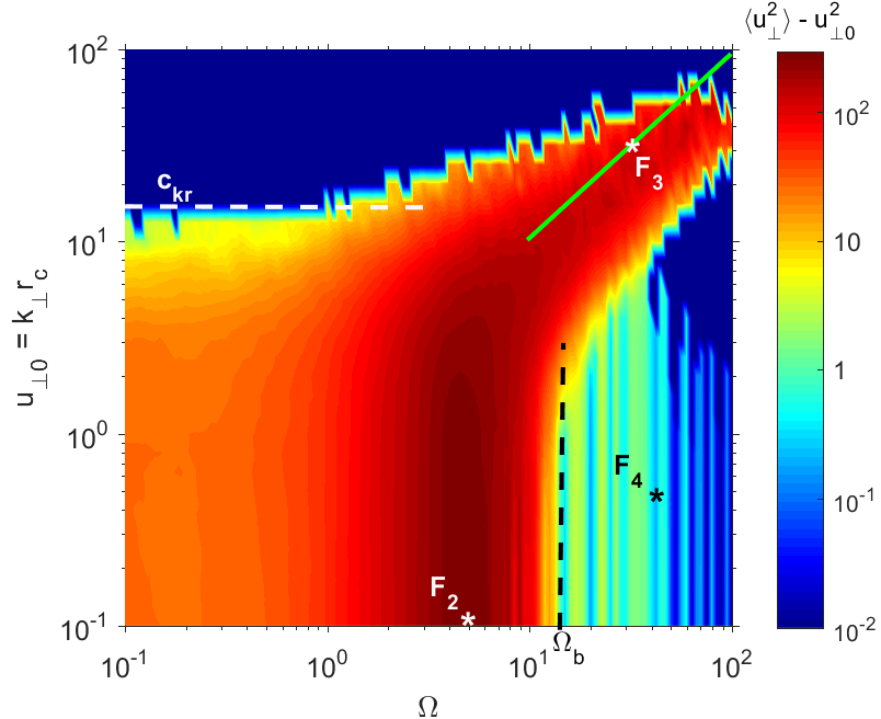
Figure 1: A colormap of stochastic energization showing the difference $\langle u_{\perp}^{2}\rangle-u_{\perp 0}^{2}$ between the normalized squared speed at the end of the simulation and the initial value $u_{\perp 0}^{2}=k_{x}^{2}r_{c}^{2}$ after 1 cyclotron period for charged particles in an electrostatic wave with normalized electric field amplitude $\widetilde{\chi}=30$. Bulk heating takes place for $\Omega\lesssim\Omega_{b}\approx 13$ (vertical dashed line) and for $u_{\perp 0}\lesssim c_{kr}\approx 15$, while for $u_{\perp 0}\gtrsim c_{kr}$, there is significant heating only for thermal velocity comparable to the wave phase velocity, or $u_{\perp 0}\sim\Omega$ in the normalized variables (diagonal green line) leading to a distribution function having a high energy tail of particles. Positions marked with asterisk refer to Figures 2, 3, and 4 where the acceleration process is studied in detail.

The system (2)-(4) is advanced in time using a Störmer-Verlet scheme (Press et al., 2007). Simulations are carried out for several values of the normalized wave frequency $\Omega$ in the range $10^{-1}$ to $10^{2}$, and for the initial normalized thermal speed $u_{\perp 0}$ spanning $10^{-1}$ to $10^{2}$. The normalized amplitude of the electrostatic wave is set to $\widetilde{\chi}=30$, which is typical for lower hybrid waves measured at the Earth’s bow shock (Stasiewicz & Eliasson, 2020a). The simulations are run for a relatively short time of one cyclotron period, motivated by the observations of rapid ion heating at the bow shock. The normalized mean squared speeds $\langle u_{\perp}^{2}\rangle=k_{\perp}^{2}\langle v_{\perp}^{2}\rangle/\omega_{c}^{2}$ at the end of the simulations are calculated as

$$\langle u_{\perp}^{2}\rangle=\frac{1}{M}\sum_{l=1}^{M}(u_{x,l}^{2}+u_{y,l}^{2}).$$ (8)

Figure 1 shows a color plot of the difference $\langle u_{\perp}^{2}\rangle-u_{\perp 0}^{2}$ between the normalized squared speed $\langle u_{\perp}^{2}\rangle$ at the end of the simulation and the initial value $u_{\perp 0}^{2}=k_{\perp}^{2}r_{c}^{2}$.

It can be seen that the bulk heating region is most intense for frequencies $\Omega<\Omega_{b}\sim 13$. For protons this limit corresponds to frequencies one-third of the lower hybrid frequency ($\Omega_{lh}\approx 43$), and for wavelengths satisfying

$$k_{\perp}r_{c}<c_{kr}\sim 15;\qquad r_{c}\lesssim 2\lambda_{\perp}.$$ (9)

Thus, the stochastic acceleration of bulk plasma disappears, when the thermal particle gyroradius becomes larger than two wavelengths. The frequency limit, $\Omega_{b}$, and also $c_{kr}$ limit would shift to larger values for maps computed with larger $\widetilde{\chi}\;$(Stasiewicz & Eliasson, 2020a).

There is also a region of the acceleration of suprathermal particles from the tail of the distribution function that occurs along the green line $k_{\perp}r_{c}\approx\Omega$, for $\Omega\gtrsim 10$ as seen in Figure 1. Particles on this line, hereafter referred to as the acceleration lane, have gyration speed $v_{\perp 0}$ that matches the phase speed of waves (Fukuyama et al., 1977; Karney, 1979)

$$v_{\perp 0}\approx r_{c}\omega_{c}=\omega/k_{\perp}=f\lambda_{\perp},$$ (10)

which links $v_{\perp}$ with electrostatic waves ($f,\lambda_{\perp}$) that can accelerate these particles. While the bulk heating is done stochastically for all particles satisfying (9), the perpendicular acceleration to high velocities along the acceleration lane (10) is selective and requires some speed and phase matching.

2.1 The physics of the E$\times$B wave heating

In order to understand the physics of the stochastic energization we have analyzed individual particle trajectories for cases marked ’$F_{2}$’, ’$F_{3}$’, and ’$F_{4}$’ in Figure 1. Figure 2 shows a solution of Equations (2)-(4) for one particle with speed $u_{x0}=0.1$ and $u_{y0}=0$ injected into a wave at frequency $\Omega=5$ and amplitude $\mbox{$\widetilde{\chi}\;$}=30$ in the bulk heating region marked as ’$F_{2}$’ in Figure 1. The particle energy is increased by factor 10⁴ within a half oscillation period of the electrostatic wave, corresponding to 1/10 gyroperiod. In the beginning, the particle makes cyclotron motion with small velocity $u_{\perp}=0.1$ (not visible in the plot) until $t=0$, when the wave is switched on. The velocity $u_{x}(t)$ shows polarization drift response $\propto dE_{x}/dt$, in the wave electric field, before resuming the cyclotron motion after one gyroperiod. The velocity $u_{y}$ increases with time as the E$\times$B velocity $v_{y}(t)=-\widetilde{E}_{x}(t,x)/B_{0}$ to the maximum value in the normalized variables $u_{y}\approx(E_{x0}/B_{0})(k_{x}/\omega_{c})\equiv\mbox{$\widetilde{\chi}\;$}$.

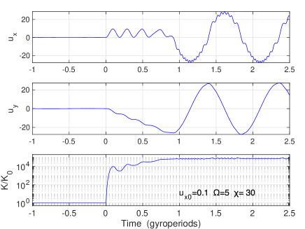
Figure 2: Acceleration of a particle in the bulk heating region (marked as ’$F_{2}$’ in the colormap) with initial velocity $u_{x0}=k_{x}r_{c}=0.1,\;u_{y0}=0$ by wave $\Omega=5$ and $\mbox{$\widetilde{\chi}\;$}=30$ . The wave is switched on at $t=0$. Panels show velocity components $u_{x}$, $u_{y}$, and the kinetic energy ratio $K/K_{0}$. Energy increase by a factor of 10⁴ is achieved within half of the wave period, or 1/10 of the gyroperiod.

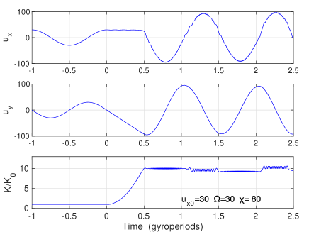
Figure 3: The particle exiting Figure 2 with $u_{x0}=30$ encounters new wave $\Omega=30,\;\mbox{$\widetilde{\chi}\;$}=80$ and is energized by a factor of 10 within half of the gyroperiod. The position in the colormap is marked as ’$F_{3}$’.

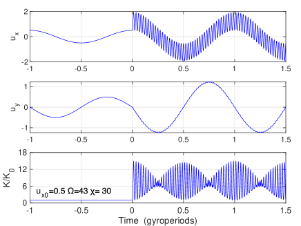
Figure 4: Acceleration of a low energy particle with $u_{x0}=0.5$ by a lower hybrid wave $\Omega=43,\;\mbox{$\widetilde{\chi}\;$}=30$. A proton is accelerated by a factor of 6 within 1/40 of the gyroperiod. The position in the colormap is marked as ’$F_{4}$’.

The mechanism described above will be called ’$\chi$-acceleration’, or the ’E$\times$B acceleration’, because the maximum acceleration capacity corresponds to the value of $\widetilde{\chi}\;$, in normalized units, or to the E$\times$B velocity computed with the wave electric field, i.e., $\widetilde{V}_{E}=\widetilde{E}_{\perp}/B$ in physical units. This limiting value for the acceleration was previously found by Sugihara & Midzuno (1979) and Dawson et al. (1983), who analyzed the same equations (2)-(4) in the wave frame. This mechanism has been also used in simulations of ion heating by large amplitude magnetosonic waves by Lembege et al. (1983). The energization capacity is then

$$K_{E}\lesssim\frac{m}{2}[v_{\perp 0}^{2}+(\widetilde{E}_{\perp}/B)^{2}],$$ (11)

which is mass dependent. This equation is a general limit for the perpendicular acceleration of particles in quasi-parallel and quasi-perpendicular shocks as will be shown in section 3. It is applicable both to the bulk heating region, where $v_{\perp 0}=v_{T}$ is the thermal speed of particles, and also to the acceleration lane, where $v_{\perp 0}$ of suprathermal particles corresponds to the wave phase speed, or equivalently to $u_{\perp 0}=k_{\perp}r_{c}\sim\Omega$.

The acceleration capacity offered by equation (11) can be estimated from the electric field measured on the Magnetospheric Multiscale (MMS) spacecraft (Burch et al., 2016) by Ergun et al. (2016); Lindqvist et al. (2016). In shocks the measured field typically exceeds 70 mV m^-1 for frequencies $\gtrsim 64$ Hz (available only in burst mode), with peak values of 300 mV m^-1. The magnetic field provided by Russell et al. (2016) can drop below 5 nT in the foreshock, so the resulting velocity could be larger than $\widetilde{V}_{E}=\widetilde{E}/B\gtrsim 14,000$ km s^-1. With this value for speed we obtain a minimum of 1 MeV as the capacity of the $\chi$-acceleration for protons at the bow shock.

The amplitudes of the wave electric field $\widetilde{E}$ and of $\widetilde{\chi}\;$increase with frequency, which makes higher frequency waves more suitable for acceleration of particles to higher energies. The lower frequency waves $\Omega<1$ ( $f<f_{c}=\omega_{c}/2\pi$) are inefficient accelerators because of smaller amplitudes. They also require interaction times of a few cyclotron periods, but long coherent wave trains are unlikely to occur in turbulent shock plasma.

2.2 The acceleration lane and the polarization drift

The particle accelerated to $u_{x}=30$ in the first step can encounter a new wave on the acceleration lane with frequency $\Omega=30$ and get additional energization as shown in Figure 3. The second wave with $\mbox{$\widetilde{\chi}\;$}=80$ would energize the particle by a factor of $10$ within a half gyroperiod. In this case $u_{x}(t)$ is constant, and $u_{y}(t)$ increases steady to the value of $\widetilde{\chi}\;$, i.e., to the E$\times$B speed in the wave field, until the cyclotron motion is resumed after $t=0.5$. The second wave could be in any direction. The only requirement is that the phase speed of wave matches the perpendicular speed of a particle on an arbitrary phase of the gyration. The acceleration could continue along the acceleration lane, but it requires larger $\Omega$ and larger $\widetilde{\chi}\;$values on each subsequent step. The acceleration works equally well for a conglomerate of waves with different frequencies and random phases (Stasiewicz et al., 2021).

By checking the effectiveness of the $\chi$-acceleration for different input parameters it is found that around the acceleration lane ($u_{\perp 0}\sim\Omega$) the approximate energization rate is

$$K/K_{0}\sim 1+(\mbox{$\widetilde{\chi}\;$}/u_{\perp 0})^{2},$$ (12)

which could continue to arbitrary high velocities $u_{\perp}$, providing there exist waves with sufficiently high amplitudes $\mbox{$\widetilde{\chi}\;$}\sim u_{\perp}$. The above expression is in fact equivalent to equation (11) derived in a different way.

Yet another type of acceleration occurs for low energy particles in waves $\Omega>\Omega_{b}$, around the lower hybrid frequency $\Omega\approx 43$ (position ’$F_{4}$’ in Figure 1) . It is seen in Figure 4 that a proton with velocity $u_{x0}=0.5$ is rapidly accelerated by an average factor of 6 within the wave period (1/40 of the cyclotron period), but it executes quivering motion related to the polarization drift seen in panel $u_{x}$. This means that the frequency $\Omega_{b}$ in Figure 1 represents in fact the boundary between the strong E$\times$B drift response for $\Omega<\Omega_{b}$, and a weaker polarization drift response for $\Omega>\Omega_{b}$.

Equation (10) implies that particles with perpendicular energy $K_{0}$ and mass $m$ are on the acceleration lane when

$$K_{0}=\frac{m}{2}f^{2}\lambda_{\perp}^{2}.$$ (13)

A handy formula for ions with atomic mass $A=m_{i}/m_{p}$ is

$$K_{0\mathrm{[keV]}}\approx 10Af_{\mathrm{[kHz]}}^{2}\lambda_{\perp\mathrm{[km]}}^{2}$$ (14)

which applies also for electrons with $A=1/1836$. Using this expression we can find, for example, that protons with energy 1 keV could be accelerated by waves $f=10$ Hz, $\lambda_{\perp}\approx 33$ km, which are in the lower hybrid range. On the other hand, protons at energy 1000 keV would interact with waves $f=1$ kHz and $\lambda_{\perp}\approx 10$ km, which could be found in the ECD frequency range. Oxygen ions ($A=16$) at energy of 16 MeV would interact with the same waves ($f\approx 1$ kHz and $\lambda_{\perp}\approx 10$ km) as 1 MeV protons.

The wave phase velocity $f\lambda_{\perp}=\omega/k_{\perp}$ in (13) determines the energy of particles prone to the acceleration by waves. The LHD waves have maximum frequency $\omega_{lh}=(\omega_{ce}\omega_{ci})^{1/2}$ and wavenumbers $k_{\perp}(r_{e}r_{i})^{1/2}\sim 1$, as shown by Daughton (2003) and Umeda & Nakamura (2018), so the phase speed of LHD waves is $v_{ph}=f\lambda_{\perp}\sim(v_{Te}v_{Ti})^{1/2}$. Here, $v_{Te}=(2T_{e}/m_{e})^{1/2}$ is the electron thermal speed, $v_{Ti}=(2T_{i}/m_{i})^{1/2}$ is the ion thermal speed and the gyroradii are: $r_{e}=v_{Te}/\omega_{ce},\>r_{i}=v_{Ti}/\omega_{ci}$. This gives the maximum energy of particles accelerated by LHD waves with $\Omega\approx\omega_{lh}/\omega_{cp}\lesssim 43$ as

$$K^{\mathrm{LHD}}\lesssim 1.5\left(\frac{m_{i}}{m_{e}}T_{e}T_{i}\right)^{1/2},$$ (15)

where the factor 1.5 is an empirical factor that fits the energy of the accelerated ions in perpendicular shocks as shown in section 3. This value can be compared with factor of 2 implied by Equation (12) when $\mbox{$\widetilde{\chi}\;$}\sim u_{\perp 0}<43$. For temperatures $T_{e}\approx 40$ eV,   $T_{i}\approx 400$ eV we obtain the proton energy $K\sim$ 8 keV, which is typically observed as the upper acceleration energy at quasi-perpendicular shocks.

2.3 Comparison with other models

The processes described in sections 2.1 and 2.2 have some components in common with the surfatron mechanism introduced by Katsouleas & Dawson (1983) for the relativistic acceleration of electrons in laser plasmas. The surfatron idea is based on work by Sagdeev (1966) and has been elaborated further in many papers (Zank et al., 1996; Shapiro et al., 2001; Ucer & Shapiro, 2001; Shapiro & Ucer, 2003; Eliasson et al., 2005). It has been also used to explain acceleration in shocks of supernova remnants (McClements et al., 2001) and acceleration of cosmic rays (Kichigin, 2013). Namely, particles can be trapped and transported in the potential well during extended time, which leads to the acceleration in the perpendicular direction until the resulting Lorentz force exceeds the electrostatic force of the wave, and the particle becomes un-trapped.

The surfing acceleration, as explained by Shapiro et al. (2001); Shapiro & Ucer (2003), applies to quasi-perpendicular shocks, where electrostatic waves propagate in the sunward, $x$-direction, while the particles are accelerated in the $y$-direction, tangentially to the shock front. The acceleration is mainly by the dc convection electric field $E_{y0}$, and partly by the wave field $E_{x}$ for trapped particles. The surfatron mechanism requires wide front of coherent waves, with several ion gyroradii width in the $y$-direction and acceleration is done after multiple ion reflections between the shock and the upstream region (Shapiro et al., 2001). The surfatron mechanism of Katsouleas & Dawson (1983) offered ’unlimited acceleration’, but because of practical impossibility to create wide front of coherent waves both in the laboratory plasma and at the turbulent bow shock, the ideas of efficient surfatron acceleration have not been confirmed experimentally. Another problem with surfing acceleration is that the wave electric field strengths are likely above the threshold for the modulational instability that leads to the breakup of the wave and eventually wave collapse. This would make turbulent field structures that destroys the phase trapping necessary for the surfatron mechanism.

In contradistinction to the cited models of surfing acceleration, the E$\times$B wave mechanism does not require extended surfing because it is coupled with the stochastic condition (1). For large $\chi$ values, energization by a factor 10⁴ can be done within the wave period $f^{-1}$ as seen in Figure 2. It corresponds to 1/40 of the proton gyroperiod for lower hybrid waves in Figure 4.

The E$\times$B wave mechanism does not require wide wavefronts as the classical surfing acceleration (Katsouleas & Dawson, 1983; Ucer & Shapiro, 2001; Shapiro & Ucer, 2003), and the acceleration can be done by bursty intermittent wave packets as observed in satellite data shown in Figure 6. It has been demonstrated recently (Stasiewicz et al., 2021) that a conglomerate of waves with a wide range of frequencies and random phases can accelerate protons from 10 eV to 100 keV within a gyroperiod. The proton energy flux obtained from simulations accurately reproduces the measured ion spectra at the bow shock.

The E$\times$B wave mechanism supported by Equation (1) operates not only at quasi-perpendicular and quasi-parallel shocks (Stasiewicz & Eliasson, 2020a, b), but also, for example, in laboratory plasma during ion heating by drift waves (McChesney et al., 1987), and in the ion heating regions of the topside ionosphere (Stasiewicz et al., 2000).

Both shock surfing acceleration and shock drift acceleration (Ball & Melrose, 2001) rely on macroscopic convection electric field to accelerate particles. The present mechanism uses only the wave electric field. The wave amplitudes measured in shocks above the lower hybrid frequency are typically 10-100 times larger than the convection field, which ensures rapid acceleration and high energization ratios. As will be shown later, it is most efficient in parallel shocks, where the average convection field is zero.

Other models require some pre-acceleration or heating, before they can be operational. The heating map in Figure 1 can explain both, a rapid heating of 10 eV particles by a factor of 10⁴, and further acceleration of 1 MeV ions along the acceleration lane. As mentioned earlier, the E$\times$B acceleration works within a fraction of the gyroperiod, while the shock surfing acceleration (Zank et al., 1996; Ucer & Shapiro, 2001; Shapiro & Ucer, 2003) requires many cyclotron periods, and the diffusive shock acceleration (Bell, 1978; Lee & Fisk, 1982) requires even much longer times.

In the next section we show measurements of waves and turbulence at quasi-perpendicular and quasi-parallel shocks, which indicate that these waves are likely to $\chi$-heat bulk of ions and also accelerate some particles to high energies by the E$\times$B mechanism presented above.

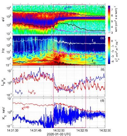
Figure 5: Quasi-perpendicular shock measured by the MMS3 spacecraft. (a) Time versus energy spectrogram of the ion differential energy flux measured by FPI. Overplotted are the electron and ion temperatures and the acceleration capacity of LHD waves given by equation (15). (b) Time versus frequency spectrogram of the $E_{y}$ (GSE) component of the electric field. Overplotted are the electron cyclotron $f_{ce}$, the lower hybrid $f_{lh}$, and the proton cyclotron $f_{cp}$. (c) The measured gradient scale of the magnetic field $L_{B}$ and of the plasma density $L_{N}$ normalized with the thermal proton gyroradius $r_{p}$. (d) The energization capacity of waves given by (11) for waves $f<20$ Hz in the lower hybrid frequency range. Overplotted is the acceleration capacity given by equation (15). Active energization and heating of ions occur within the red box.

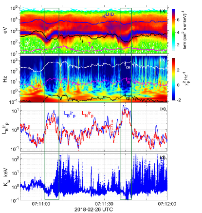
Figure 6: Quasi-parallel shock measured by the MMS3 spacecraft. (a) Ion energy flux spectrogram measured by FPI in the energy range 10 eV - 20 keV combined with EIS measurements in the energy range 20-100 keV. Overplotted are electron and ion temperatures and the acceleration capacity of LHD waves given by equation (15). (b) Time versus frequency spectrogram of $\chi_{p}$. Overplotted are the plasma frequencies: $f_{ce}$, $f_{lh}$, and $f_{cp}$. (c) Gradient scales $L_{B}$ and $L_{N}$ derived from measurements and normalized with $r_{p}$. (d) The energization capacity of waves given by (11) for waves in the measured frequency range 0-4000 Hz. Two green boxes mark two magnetic shocklets where the active ion energization does not occur.

3 Comparison with observations

Figure 5 shows 1 minute of burst-mode data from the quasi-perpendicular bow shock. This is one of 9 multiple shock encounters analyzed by Stasiewicz & Eliasson (2020a). The particle data from the Fast Plasma Investigation (FPI) (Pollock et al., 2016) shown in panel (a) are taken at position (10.2, 13.4, -1.8) $R_{E}$ GSE (geocentric solar ecliptic). The Alfvén Mach number was 7.2, the electron plasma beta $\beta_{e}\approx 1.1$, and the ion beta $\beta_{i}\approx 2.5$, on the upstream (right) side of the shock. The angle between the magnetic field and the geocentric radial direction (a proxy to the shock normal) was 124^∘. Overplotted are the ion and electron temperatures, and the acceleration capacity of LHD waves given by (15). This equation provides accurate values for the maximum energy of protons accelerated at quasi-perpendicular shocks observed by MMS.

Active heating and acceleration of ions, seen in the ion temperature and the energy spectrum in panel (a) occur within the red box, which contains the ramp and the foot of the shock. In this region, ions are accelerated up to about 4 keV. The red box coincides with the region of the smallest values of the gradient scale lengths $L_{B}=B|\nabla B|^{-1}$ for the magnetic field and $L_{N}=N|\nabla N|^{-1}$ for the electron density $N$, both normalized by the thermal ion gyroradius $r_{p}$ and shown in panel (c). The condition $L_{N}/r_{p}<(m_{p}/m_{e})^{1/4}\approx 5$ determines the onset of the lower hybrid drift (LHD) instability (Davidson et al., 1977; Drake et al., 1983; Gary, 1993), while $L_{N}/r_{p}<1$ in most of the time interval indicated by a red box in Figure 5. The gradient scales are derived directly from four point measurements using the method of Harvey (1998). It is seen that the values for $L_{N}$ derived for the cold solar wind, after 14:32:10 UTC are not reliable, and the values for $L_{B}$ should be used instead.

Almost the whole time interval in Figure 5 the plasma is unstable for the LHD instability, as seen in the wave spectrogram in panel (b) with the most intense waves in the frequency range $f_{cp}-f_{lh}$ located in the red box. These waves are indeed responsible for the ion energization through the E$\times$B mechanism presented in section 2. This can be seen in panel (d). The acceleration capacity of waves below 20 Hz derived with (11) corresponds exactly to the limiting energy of ions in panel (a), and coincides also with the other independent estimate (15). The frequencies plotted in panel (b) are proportional to $B$ so the magnetic structure of the shock can be inferred from the frequency plots. Complementary discussion and overview of data for this case can be found elsewhere (Stasiewicz & Eliasson, 2020b).

Figure 6 shows 1 minute of data from a long duration quasi-parallel shock measured by the MMS3 spacecraft. The satellite was at position (12.6, -3.9, 4.1) $R_{E}$, where the Alfvén Mach number was in the range 1-6 with the average of 3, the average electron plasma beta $\beta_{e}\sim 0.7$, and the ion beta $\beta_{i}\sim 5$. The data represents a couple of shocklets, i.e., compressions of the plasma density and of the magnetic field associated with retardation of the solar wind beam as seen in panel (a). Two shocklets are marked with green boxes. A major difference between this case and the previous one is that here ions are accelerated to up to about 100 keV, while in the quasi-perpendicular shock the ions were only accelerated to about 4 keV. In quasi-parallel shocks the acceleration of suprathermal particles extends well beyond the boundary $K^{LHD}$ as seen in panel (a).

The energization limit for the measured waves computed with (11) is shown in panel (d). We see excellent agreement between the theoretical maximum energy $\sim 100$ keV in panel (d) and the measured energy spectra in panel (a). The average gyroradius of a 40 keV proton in this time interval is 2000 km. Because of large gyroradii of energetic ions, which tap energy from intermittent waves over large spatial areas, direct spatial correlations between $\sim\,$100 keV ions in panel (a) and accelerating waves in panel (d) are not expected. Such correlations do exist for low energy protons in Figure 5, in the red box.

The large difference in the maximum acceleration between quasi-perpendicular and quasi-parallel shocks appears to be related to the interaction time with waves. In perpendicular shocks, the solar wind is rapidly convected across the shock so the acceleration is done by LHD waves up to the limit (15), or to the limit (11) computed for lower hybrid waves only ($f<20$ Hz), during a short time comparable to one gyroperiod. This observation indicates that the surfatron mechanism does not operate at quasi-perpendicular shocks. If the ions were reflected from the shock and remained longer time by surfing in the foot-ramp area they would have been accelerated to the limit (11), i.e. $\sim 100\,$keV also in quasi-perpendicular shocks, which is not observed.

In parallel shocks, energetic ions meander between the shocklets in the upstream region and repetitively interact with higher frequency waves at increasing frequencies during much longer times. This would stepwise increase their energy to the limit (11) through the same $\chi$-acceleration mechanism, along the acceleration lane of Figure 1.

Let us analyze waves shown in panel (b). The time versus frequency spectrogram of $\chi_{p}$ given by Equation (1) is derived from measurements of the electric field sampled at the rate 8192 s^-1. The computed values reach $\chi_{p}\approx 1800$ for higher frequency ECD waves. Details of the technique for computing $\mathrm{div}(\mathbf{E})$ from four point measurements are discussed by Stasiewicz & Eliasson (2020a, b).

Figure 6(c) shows $L_{B}/r_{p}$ and $L_{N}/r_{p}$ similar to Figure 5(c). Here, there is good agreement between the magnetic field and density length scales. The LHD waves in panel (b) are in excellent correlation with regions $L_{N}/r_{p}\lesssim(m_{p}/m_{e})^{1/4}\sim 5$, where the lower hybrid drift instability should theoretically occur.

As mentioned in section 1, the wave generation process in both cases is initiated by the density gradients associated with the quasi-perpendicular shock in Figure 5 and with quasi-parallel shocklets in Figure 6, which produce diamagnetic currents that cause first the LHD instability (Davidson et al., 1977; Gary, 1993; Daughton, 2003) which has a lower threshold than the MTS and ECD instabilities.

The wave spectrograms in Figures 5(b) and 6(b) can be divided into four frequency bands: the magnetosonic waves below $f_{cp}$, the lower hybrid drift (LHD) waves in the frequency range $f_{cp}-f_{lh}$, the modified two-stream (MTS) instability in the range $f_{lh}-f_{ce}$, and the electron cyclotron drift (ECD) waves around and above $f_{ce}$. Other wave modes like whistlers and ion acoustic waves may also contribute in the spectrograms. The displayed spectrograms are in the spacecraft frame, so there may be some mixing and overlap of modes due to the frequency Doppler shift of short wavelengths by the bulk plasma flow $\sim 250$ km s^-1.

In the frequency range $f_{cp}-f_{lh}$ there are magnetic field fluctuations, which are also observed in simulations (Daughton, 2003), in the magnetotail (Ergun et al., 2019), and at the magnetopause (Graham et al., 2019). This could mean that LHD waves coexist with ion whistler waves created in the density striations by mode conversion (Rosenberg & Gekelman, 2001; Eliasson & Papadopoulos, 2008; Camporeale et al., 2012) from LHD waves, or with magnetosonic fluctuations. Such whistler waves, propagating upstream are seen in Figure 5. Lower hybrid waves and whistlers can be also produced by ring distributions (Winske & Daughton, 2015) of ions reflected from the bow shock, but Figure 5c and analysis of similar waves in Figure 6 indicate that the driving mechanism for LHD waves at both shocks are density gradients rather than the reflected ion beams. However, the magnetosonic waves in the frequency range $f_{cp}-f_{lh}$ are equally efficient ion accelerators as demonstrated by Lembege et al. (1983); Lembege & Dawson (1984) and Ohsawa (1985).

The enhanced electric field of the LHD or magnetosonic waves produces strong E$\times$B drifts of electrons only, because the ions are not subject to this drift due to their large gyroradius in comparison to the width of drift channels. When the electron-ion drift exceeds the ion thermal speed and becomes a significant fraction of the electron thermal speed, the MTS (Wu et al., 1983; Umeda et al., 2014; Muschietti & Lembège, 2017) and ECD instabilities (Lashmore-Davies & Martin, 1973; Muschietti & Lembége, 2013; Janhunen et al., 2018) are triggered at frequencies from above $f_{lh}$ to a few harmonics of $f_{ce}$. Such waves are commonly observed at the bow shock (Wilson III et al., 2010; Breneman et al., 2013; Goodrich et al., 2018). Note the vertical striations in panels 5(b) and 6(b) that start from $\sim 0.5$ Hz (LHD instability) and extend up through the MTS and ECD instabilities to 3 kHz, indicating co-location and common origin of these instabilities. The MTS waves propagate obliquely to the magnetic field and produce parallel electric field component that may be responsible for the isotropisation of the electron distribution (Stasiewicz & Eliasson, 2020b).

The sequential triggering and co-location of the LHD-MTS-ECD instabilities can be also explained by considering the expression for the E$\times$B drift velocity for particles with gyroradius $r_{c}$ in a spatially varying electric field $E_{x}\propto\sin(k_{\perp}x)$ (Chen, 2016)

$$\mathbf{V}_{E}=\frac{\mathbf{E}\times\mathbf{B}}{B^{2}}(1-\frac{1}{4}k_{\perp}^{2}r_{c}^{2}).$$ (16)

Ions with large gyroradius would have greatly reduced E$\times$B drift velocity in comparison with small gyroradius electrons. When the ratio $\lambda_{\perp}/r_{p}\lesssim\pi$, the ion electric drift vanishes, and the sole electron drift would produce strong cross-field current that could drive the above mentioned instabilities. Actually, the conditions for the onset of the diamagnetic LHD instability on density gradients, and the complete quenching of the E$\times$B ion drift on short wavelengths are similar

$$\frac{L_{N}}{r_{p}}\sim\frac{\lambda_{\perp}}{r_{p}}\lesssim 5,$$ (17)

which means that the chain of the instabilities LHD-MTS-ECD could be enforced by steepening of magnetosonic shock waves to smaller wavelengths, even in the absence of sufficient diamagnetic currents.

One should be also aware, that the E$\times$B drift of particles (16) is a different phenomenon than the E$\times$B wave energization mechanism (11) discussed in this paper. The E$\times$B wave heating of ions starts, when the E$\times$B drift stops.

The ions accelerated by the $\chi$-mechanism in quasi-parallel shocks can diffuse through the magnetopause and form the quasi-trapped population of energetic ions inside. This idea is opposite to claims that the energetic ions observed upstream of the bow shock represent leakage of particles from the magnetosphere (Mauk et al., 2019). The dependence $\mbox{$\widetilde{\chi}\;$}\propto m/q$, and mass dependence of the energization (11,13) could explain observations that heavy ions in the C,N,O group have fluxes larger than protons at high energies (Stasiewicz et al., 2013; Turner et al., 2018). This is also consistent with observation of heavy ion temperatures $T_{i}\propto m_{i}/m_{p}$ in post-shocks of supernova remnants (Raymond et al., 2017; Miceli et al., 2019; Gedalin, 2020). However, there are also other explanations for the preferential heating of heavy ions (Zank et al., 1996, 2001; Shapiro et al., 2001).

4 Conclusions

This research is based on the well established concepts of the stochastic heating laid down in a seminal paper by Karney (1979), represented by Equation (1), and on the E$\times$B wave acceleration limit by large amplitude waves found by Sugihara & Midzuno (1979) and Dawson et al. (1983), represented by Equation (11). By combining these two concepts with multipoint MMS measurements (Burch et al., 2016) we have shown that solar wind ions are bulk heated by the stochastic mechanism (1) both in quasi-perpendicular and in quasi-parallel shocks confirming the previous results of Stasiewicz & Eliasson (2020a, b). The perpendicular $\chi$-heating is a rapid process and may be accomplished within a fraction of a gyroperiod. Selected suprathermal particles with perpendicular gyration velocity equal to the phase speed of electrostatic waves $v_{\perp}\approx\omega/k_{\perp}$ can be accelerated to velocities of the E$\times$B drift in the wave field, $\widetilde{V}_{E}=\widetilde{E}_{\perp}/B$. The acceleration requires waves with the stochastic heating parameter $\mbox{$\widetilde{\chi}\;$}=(\widetilde{E}_{\perp}/B)(k_{\perp}/\omega_{c})\gg 1$ and occurs in discrete steps on intermittent waves observed in shocks. The process could bring some ions to the speed of $\sim 14,000$ km s^-1 or 1 MeV for protons, which is possible in quasi-parallel bow shocks where $\widetilde{E}\gtrsim 70$ mV m^-1 and $B\lesssim 5$ nT are observed. In the case analyzed in this paper protons are accelerated to $\sim 100$ keV and the theoretical prediction matches the measurements.

In collisionless shocks, waves that accelerate ions are produced by the three cross-field current-driven LHD, MTS, and ECD instabilities, in the frequency range $f_{cp}-nf_{ce}$, which are seen in Figure 6(b). The instabilities are cascade-triggered by diamagnetic currents induced by the density gradients created both in perpendicular shocks and in shocklets that form parallel shocks.

The short interaction time with waves at perpendicular shocks limits the maximum energy of protons accelerated by LHD waves to $\sim 10$ keV, while the multi-step acceleration by higher frequency waves $f_{lh}-nf_{ce}$ in parallel shocks can bring some ions to the MeV energy range. The general expression (11) provides an explanation of the observed maximum energy of ions accelerated in shocks of arbitrary configuration.

It is suggested that ions accelerated in quasi-parallel shocks to hundreds keV diffuse into the magnetosphere and form the quasi-trapped energetic ion population.

The $\chi$- or E$\times$B -mechanism accelerates heavy ions to energies proportional to the atomic mass number, which is consistent with satellite observations upstream of the bow shock and also with observations of ion temperatures in post-shocks of supernova remnants.

References

- Balikhin et al. (1993) Balikhin, M., Gedalin, M., & Petrukovich, A. 1993, Phys. Rev. Lett., 70, 1259, doi: 10.1103/PhysRevLett.70.1259
- Ball & Melrose (2001) Ball, L., & Melrose, D. B. 2001, Publications of the Astronomical Society of Australia, 18, 361, doi: 10.1071/AS01047
- Bell (1978) Bell, A. R. 1978, MNRAS, 182, 147, doi: 10.1093/mnras/182.2.147
- Breneman et al. (2013) Breneman, A. W., Cattell, C. A., Kersten, K., et al. 2013, JGR, 118, 7654, doi: 10.1002/2013JA019372
- Burch et al. (2016) Burch, J. L., Moore, R. E., Torbert, R. B., & Giles, B. L. 2016, Space Sci. Rev., 199, 1, doi: 10.1007/s11214-015-0164-9
- Burgess et al. (2012) Burgess, D., Möbius, E., & Scholer, M. 2012, Space Sci. Rev., 173, 5, doi: 10.1007/s11214-012-9901-5
- Camporeale et al. (2012) Camporeale, E., Delzanno, G. L., & Colestock, P. 2012, JGR, 117, A10315, doi: 10.1029/2012JA017726
- Chen (2016) Chen, F. F. 2016, Introduction to Plasma Physics and Controlled Fusion (Springer)
- Daughton (2003) Daughton, W. 2003, Phys. Plasmas, 10, 3103, doi: 10.1063/1.1594724
- Davidson et al. (1977) Davidson, R. C., Gladd, N. T., Wu, C., & Huba, J. D. 1977, Phys. Fluids, 20, 301, doi: 10.1063/1.861867
- Dawson et al. (1983) Dawson, J. M., Decyk, V. K., Huff, R. W., et al. 1983, Phys. Rev. Lett., 50, 1455, doi: 10.1103/PhysRevLett.50.1455
- Drake et al. (1983) Drake, J. F., Huba, J. D., & Gladd, N. T. 1983, Phys. Fluids, 26, 2247, doi: 10.1063/1.864380
- Eastwood et al. (2005) Eastwood, J. P., Lucek, E. A., Mazelle, C., et al. 2005, Space Science Reviews, 118, 41, doi: 10.1007/s11214-005-3824-3
- Eliasson et al. (2005) Eliasson, B., Dieckmann, M. E., & Shukla, P. K. 2005, New Journal of Physics, 7, 136, doi: 10.1088/1367-2630/7/1/136
- Eliasson & Papadopoulos (2008) Eliasson, B., & Papadopoulos, K. 2008, J. Geophys. Res., 113, A09315, doi: 10.1029/2008JA013261
- Ergun et al. (2016) Ergun, R. E., Tucker, S., Westfall, J., et al. 2016, Space Sci. Rev., 199, 167, doi: 10.1007/s11214-014-0115-x
- Ergun et al. (2019) Ergun, R. E., Hoilijoki, S., Ahmadi, N., et al. 2019, JGR, 124, 10085, doi: 10.1029/2019JA027275
- Fermi (1949) Fermi, E. 1949, Phys. Rev., 75, 1169, doi: 10.1103/PhysRev.75.1169
- Fukuyama et al. (1977) Fukuyama, A., Momota, H., Itatani, R., & Takizuka, T. 1977, Phys. Rev. Lett., 38, 701, doi: 10.1103/PhysRevLett.38.701
- Gary (1993) Gary, S. P. 1993, Theory of space plasma microinstabilities (Cambridge University Press)
- Gedalin (2020) Gedalin, M. 2020, The Astrophysical Journal, 900, 171, doi: 10.3847/1538-4357/abaa49
- Goodrich et al. (2018) Goodrich, K. A., Ergun, R., Schwartz, S. J., et al. 2018, J. Geophys. Res., 123, 9430, doi: 10.1029/2018JA025830
- Graham et al. (2019) Graham, D. B., Khotyaintsev, Y. V., Norgren, C., et al. 2019, JGR: Space Physics, 124, 8727, doi: 10.1029/2019JA027155
- Greenstadt et al. (1995) Greenstadt, E. W., Le, G., & Strangeway, R. J. 1995, Adv. Space Phys., 15, 71, doi: 10.1016/0273-1177(94)00087-H
- Harvey (1998) Harvey, C. C. 1998, in Analysis Methods for Multi-spacecraft Data, ed. G. Paschmann & P. W. Daly, Vol. SR-001 ISSI Reports (ESA), 307–322
- Janhunen et al. (2018) Janhunen, S., Smolyakov, A., Sydorenko, D., et al. 2018, Physics of Plasmas, 25, 082308, doi: 10.1063/1.5033896
- Karney (1979) Karney, C. F. F. 1979, Phys. Fluids, 22, 2188, doi: 10.1063/1.862512
- Katsouleas & Dawson (1983) Katsouleas, T., & Dawson, J. M. 1983, Phys. Rev. Lett., 51, 392, doi: 10.1103/PhysRevLett.51.392
- Kichigin (2013) Kichigin, G. 2013, Advances in Space Research, 51, 309, doi: 10.1016/j.asr.2011.10.018
- Lashmore-Davies & Martin (1973) Lashmore-Davies, C., & Martin, T. 1973, Nuclear Fusion, 13, 193, doi: 10.1088/0029-5515/13/2/007
- Lee & Fisk (1982) Lee, M. A., & Fisk, L. A. 1982, Space Sci. Rev., 32, 205, doi: 10.1007/BF00225185
- Lembege & Dawson (1984) Lembege, B., & Dawson, J. M. 1984, Phys. Rev. Lett., 53, 1053, doi: 10.1103/PhysRevLett.53.1053
- Lembege et al. (1983) Lembege, B., Ratliff, S. T., Dawson, J. M., & Ohsawa, Y. 1983, Phys. Rev. Lett., 51, 264, doi: 10.1103/PhysRevLett.51.264
- Lindqvist et al. (2016) Lindqvist, P. A., Olsson, G., Torbert, R. B., et al. 2016, Space Sci. Rev., 199, 137, doi: 10.1007/s11214-014-0116-9
- Liu et al. (2016) Liu, T. Z., Turner, D. L., Angelopoulos, V., & Omidi, N. 2016, JGR, 121, 5489, doi: 10.1002/2016JA022461
- Mauk et al. (2019) Mauk, B. H., Cohen, I. J., Haggerty, D. K., et al. 2019, JGR, 124, 5539, doi: 10.1029/2019JA026626
- McChesney et al. (1987) McChesney, J. M., Stern, R., & Bellan, P. M. 1987, Phys. Rev. Lett., 59, 1436, doi: 10.1103/PhysRevLett.59.1436
- McClements et al. (2001) McClements, K. G., Dieckmann, M. E., Ynnerman, A., Chapman, S. C., & Dendy, R. O. 2001, Phys. Rev. Lett., 87, 255002, doi: 10.1103/PhysRevLett.87.255002
- Miceli et al. (2019) Miceli, M., Orlando, S., Burrows, D. N., et al. 2019, Nature Astronomy, 3, 236, doi: 10.1038/s41550-018-0677-8
- Muschietti & Lembége (2013) Muschietti, L., & Lembége, B. 2013, J. Geophys. Res., 118, 2267, doi: 10.1002/jgra.50224
- Muschietti & Lembège (2017) Muschietti, L., & Lembège, B. 2017, Annales Geophysicae, 35, 1093, doi: 10.5194/angeo-35-1093-2017
- Ohsawa (1985) Ohsawa, Y. 1985, Physics of Fluids, 28, 2130, doi: 10.1063/1.865394
- Otsuka et al. (2018) Otsuka, F., Matsukiyo, S., Kis, A., Nakanishi, K., & Hada, T. 2018, ApJ, 853, 117, doi: 10.3847/1538-4357/aaa23f
- Pollock et al. (2016) Pollock, C., Moore, T., Jacques, A., et al. 2016, Space Sci. Rev., 199, 331, doi: 10.1007/s11214-016-0245-4
- Press et al. (2007) Press, W. H., Teukolsky, S. A., Vetterling, W. T., & Flannery, B. P. 2007, Numerical Recipes: The Art of Scientific Computing (Cambridge University Press, New York)
- Raymond et al. (2017) Raymond, J. C., Winkler, P. F., Blair, W. P., & Laming, J. M. 2017, The Astrophysical Journal, 851, 12, doi: 10.3847/1538-4357/aa998f
- Rosenberg & Gekelman (2001) Rosenberg, S., & Gekelman, W. 2001, J. Geophys. Res., 106, 28,867, doi: 10.1029/2000JA000061
- Russell et al. (2016) Russell, C. T., Anderson, B. J., Baumjohann, W., et al. 2016, Space Sci. Rev., 199, 189, doi: 10.1007/s11214-014-0057-3
- Sagdeev (1966) Sagdeev, R. Z. 1966, Reviews of Plasma Physics, 4, 23
- Shapiro et al. (2001) Shapiro, V. D., Lee, M. A., & Quest, K. B. 2001, Journal of Geophysical Research: Space Physics, 106, 25023, doi: https://doi.org/10.1029/1999JA000384
- Shapiro & Ucer (2003) Shapiro, V. D., & Ucer, D. 2003, Planet. Space Sci., 51, 665, doi: 10.1016/S0032-0633(03)00102-8
- Stasiewicz (2020) Stasiewicz, K. 2020, MNRAS, 496, L133, doi: 10.1093/mnrasl/slaa090
- Stasiewicz & Eliasson (2020a) Stasiewicz, K., & Eliasson, B. 2020a, The Astrophysical Journal, 903, 57, doi: 10.3847/1538-4357/abb825
- Stasiewicz & Eliasson (2020b) —. 2020b, The Astrophysical Journal, 904, 173, doi: 10.3847/1538-4357/abbffa
- Stasiewicz et al. (2021) Stasiewicz, K., Eliasson, B., Cohen, I. J., Turner, D. L., & Ergun, R. E. 2021, JGR, submitted
- Stasiewicz et al. (2000) Stasiewicz, K., Lundin, R., & Marklund, G. 2000, Physica Scripta, T84, 60, doi: 10.1238/physica.topical.084a00060
- Stasiewicz et al. (2013) Stasiewicz, K., Markidis, S., Eliasson, B., Strumik, M., & Yamauchi, M. 2013, Europhys. Lett., 102, 49001, doi: 10.1209/0295-5075/102/49001
- Sugihara & Midzuno (1979) Sugihara, R., & Midzuno, Y. 1979, Journal of the Physical Society of Japan, 47, 1290, doi: 10.1143/JPSJ.47.1290
- Thomsen et al. (1988) Thomsen, M. F., Gosling, J. T., Bame, S. J., et al. 1988, Journal of Geophysical Research: Space Physics, 93, 11311, doi: 10.1029/JA093iA10p11311
- Turner et al. (2018) Turner, D. L., Wilson, L. B., Liu, T. Z., et al. 2018, Nature, 561, 206, doi: 10.1038/s41586-018-0472-9
- Ucer & Shapiro (2001) Ucer, D., & Shapiro, V. D. 2001, Phys. Rev. Lett., 87, 075001, doi: 10.1103/PhysRevLett.87.075001
- Umeda et al. (2014) Umeda, T., Kidani, Y., Matsukiyo, S., & Yamazaki, R. 2014, Physics of Plasmas, 21, 022102, doi: 10.1063/1.4863836
- Umeda & Nakamura (2018) Umeda, T., & Nakamura, T. K. M. 2018, Physics of Plasmas, 25, 102109, doi: 10.1063/1.5050542
- Vranjes & Poedts (2010) Vranjes, J., & Poedts, S. 2010, MNRAS, 408, 1835, doi: 10.1111/j.1365-2966.2010.17249.x
- Wilson III et al. (2010) Wilson III, L. B., Cattell, C. A., Kellogg, P. J., et al. 2010, J. Geophys. Res., 115, A12104, doi: 10.1029/2010JA015332
- Winske & Daughton (2015) Winske, D., & Daughton, W. 2015, Physics of Plasmas, 22, 022102, doi: 10.1063/1.4906889
- Wu et al. (1983) Wu, C. S., Zhou, Y. M., Tsai, S.-T., et al. 1983, The Physics of Fluids, 26, 1259, doi: 10.1063/1.864285
- Zank et al. (1996) Zank, G. P., Pauls, H. L., Cairns, I. H., & Webb, G. M. 1996, J. Geophys. Res., 101, 457, doi: 10.1029/95JA02860
- Zank et al. (2001) Zank, G. P., Rice, W. K. M., le Roux, J. A., & Matthaeus, W. H. 2001, The Astrophysical Journal, 556, 494, doi: 10.1086/322238