Integrated Optimization of Heterogeneous-Network Management and the Elusive Role of Macrocells

Abstract

We consider heterogeneous wireless networks in the physical interference model and introduce a new formulation of the mixed-integer nonlinear programming problem that addresses base-station activation and many-to-many associations while minimizing power consumption. We also introduce HetNetGA, a genetic algorithm that can tackle the problem without any approximations. Though unsuitable for practical deployment, HetNetGA enables the investigation of such networks’ true possibilities. Results for scenarios involving both macrocells and picocells often align with what is expected, but sometimes are unexpected and essentially point to the need to better understand the role of macrocells in helping provide capacity while remaining energetically advantageous.

Keywords: Heterogeneous wireless networks, physical interference model, capacity allocation, power optimization.

1 Introduction

In order to meet the rapidly increasing demand for wireless capacity, a current tenet is that future-generation networks will have to rely on heterogeneity to grow. That is, every large base station (macrocell) deployed will have to be accompanied by a number of small base stations (picocells) spread amid users to improve capacity. The resulting network density will make the problems of managing interference, meeting capacity demands, and saving power not only more pressing but also more tightly coupled with one another and consequently harder to solve. Because of the many trade-offs involved in all decisions related to tackling these problems, at least some of their key aspects will likely be handled as a single entity. These include deciding which base stations to be turned on and which associations to establish between base stations and users. Of course, such decisions will always have to take into account the way the available spectrum is handled so that, in the end, the resulting contributions to network capacity are as strong as possible.

In the last few years, a number of works have addressed, with varying degrees of detail and success, the formulation and solution of optimization problems targeting more than one of those aspects concomitantly (cf. [1, 2, 3, 4, 5, 6] as representative examples). While most of them differ significantly from one another, they all share some important features, including optimization problems of a mixed nature (integer and continuous) that are handled only after undergoing approximations or having their feasible sets substantially reduced through the adoption of a limited set of so-called “patterns.” Moreover, it is generally unclear how the signal-to-interference-plus-noise ratio (SINR) threshold that is typical of the physical interference model is handled. In some cases, results are downright irreproducible.

Here we address the problem of minimizing a network’s power consumption while handling the SINR threshold appropriately, determining which base stations to be turned on as well as associations between base stations and users, and meeting user demands for capacity. Each base station can be associated with multiple users, and conversely each user with multiple base stations. To the best of our knowledge, ours is a complete formulation that stands apart from previous ones in at least one feature. In particular, our approach is unique in that we handle the resulting optimization problem, with all its integralities and resulting nonlinearities, as it comes. Instead of bending its intrinsic combinatorial nature to fit some optimization method of choice, we leverage the inherently stochastic, parallel nature of evolutionary methods and use a genetic algorithm within a simple exploratory methodology. We present results, all reproducible, in some scenarios.

Some of these results fall smoothly in line with what has become expected of heterogeneous wireless networks. This includes the effect of increased bit-rate demands on power consumption as well as on feasibility. Others have been unexpected, suggesting that the role of macrocells in such networks may be less clear than generally assumed thus far. In particular, for the network model and parameters used, we have been unable to unambiguously pinpoint a situation in which the combined use of macrocells and picocells would achieve feasibility while using picocells alone would not. That is, we have found no situation in which the use of macrocells would be energetically advantageous.

2 Contributions

Minimizing power consumption while at the same time deciding which base stations to be turned on, deciding which associations between base stations and users to establish, and ensuring that user demands for capacity are all met usually amounts to a daunting problem, full of nonlinearities and often non-differentiabilities as well. Solving this problem lies at the heart of heterogeneous-network management, so for practical deployment both network models and the algorithms to be used must be simplified in order for efficiency and scalability to be achieved. The downside of such simplifications is that the operational decisions they lead to may fail to save as much power as possible or to meet user demands when they could be met. Thus, while reconciling efficiency and scalability with solution quality is unavoidably fraught with difficult trade-offs, the need remains for approaches that do not target practical deployment but rather the detailed study of a network’s true properties. In this letter we contribute one such approach by introducing a complete model (in Section 3) and a formulation of the associated optimization problem that makes no simplifications (in Section 4, with the appropriate solution methodology given in Section 5).

Our model is complete in the sense that it incorporates crucial elements omitted from previous models. Most notable of all is a clear treatment of how SINR thresholds are handled for proper decoding. This is lacking in previous models [1, 2, 3, 4, 5, 6], which may result in poor interference coordination. Our model also provides for the determination of base-station activation (unlike [4]) and which users to associate with which base stations in a many-to-many fashion (unlike [4], where associations are not considered at all, and unlike [3, 5, 6], where associations are not many-to-many). As for simplifications to the optimization problem, our approach improves on previous ones by considering the model’s complete domain (unlike [1, 2, 5], where restrictions specified by the “patterns” mentioned in Section 1 or similar combinatorial structures are imposed), and by completely shunning any form of smoothing (unlike [1, 6], where integralities are relaxed, and unlike [4], where the functions involved are approximated) and any form of problem breakup (unlike [3]). Importantly, we have taken every possible precaution to make sure the experimental setup laid down in Section 5 is fully reproducible. This, too, is pointedly unlike some of the previous works (most notably the one in [1], whose results are hardly reproducible even at the level of how base stations and users are deployed).

These contributions have led to the one we consider to be most important, viz., a clear demonstration that by looking into the model’s unaltered characteristics it is possible to glean some properties that thus far have remained unobserved (or at least unreported). Specifically, for a reasonable set of parameter choices the results we give in Section 6 call for a better look into the role of macrocells in heterogeneous wireless networks.

3 Network model

We consider a set $B$ of base stations and a set $K$ of receivers. For $P_{b}$ the power with which base station $b\in B$ transmits, and assuming that all transmissions take place outdoors, the power $R_{bk}$ that reaches receiver $k\in K$ is

$$R_{bk}=P_{b}L_{b}^{-1}d_{bk}^{-\tau_{b}},$$ (1)

where $L_{b}$ accounts for antenna- and frequency-related losses (as well as for frequency- or distance-unit conversion), $d_{bk}$ is the Euclidean distance between $b$ and $k$, and $\tau_{b}>2$ determines how power decays with distance. We consider downlink communication exclusively and assume that receivers are capable of multi-packet reception, i.e., of handling transmissions from multiple base stations concomitantly. We model this in the manner of (uplink) CDMA over a narrowband $N$ and a wideband $W$, therefore with processing gain $G=W/N$ [7].

For $B_{\mathrm{on}}\subseteq B$ the set of base stations currently turned on and $b\in B_{\mathrm{on}}$, the SINR at receiver $k$ is

$$\mathrm{SINR}_{bk}=\frac{GR_{bk}}{\gamma_{0}W+\sum_{b^{\prime}\in B_{\mathrm{on}}\setminus\{b\}}R_{b^{\prime}k}},$$ (2)

where $\gamma_{0}$ is the noise-floor spectral density. Decoding becomes possible whenever

$$\mathrm{SINR}_{bk}\geq\beta,$$ (3)

where $\beta>1$ is a parameter related to a receiver’s decoding capabilities, assumed the same for all receivers.

If decoding is possible, we say that base station $b$ and receiver $k$ can become associated with each other. In this case, the maximum capacity $C_{bk}$ for transmissions from $b$ to $k$ is given by

$$C_{bk}=N\log_{2}(1+\mathrm{SINR}_{bk}).$$ (4)

Moreover, the maximum number $n_{\mathrm{max}}$ of concomitant associations for a given receiver is related to $G$ and $\beta$ as in

$$n_{\mathrm{max}}<1+\frac{G}{\beta},$$ (5)

so $n_{\mathrm{max}}>1$ requires $\beta<G$.

At any given time, the total capacity provided by the network depends on how much each of the base stations in $B_{\mathrm{on}}$ can provide individually. It also depends on the current associations in the network. Clearly, any base station $b\in B$ can always transmit as many bits per second as given by the greatest $C_{bk}$ over any subset of $K$ (since the expression in Eq. (4) comes from $b$ and $k$ being associated with each other). That is, letting $K_{b}\subseteq K$ be the set of receivers currently associated with base station $b\in B_{\mathrm{on}}$, the transmission capacity of base station $b$ is always at least $\max_{k\in K_{b}}\alpha_{bk}C_{bk}$, where $\alpha_{bk}$ is the fraction of time base station $b$ spends transmitting to receiver $k\in K_{b}$. On the receivers’ side, the total capacity available to receiver $k$ is $\sum_{b\in B_{k}}\alpha_{bk}C_{bk}$, where $B_{k}\subseteq B_{\mathrm{on}}$ is the set of base stations currently associated with $k$. Naturally,

$$\sum_{k\in K_{b}}\alpha_{bk}\leq 1$$ (6)

and $|B_{k}|\leq n_{\mathrm{max}}$ hold at all times, respectively for every $b\in B_{\mathrm{on}}$ and every $k\in K$. Additionally, meeting some demand $d_{k}$ at receiver $k$ requires

$$\sum_{b\in B_{k}}\alpha_{bk}C_{bk}\geq d_{k}.$$ (7)

4 Mathematical formulation

The problem we address is the determination of set $B_{\mathrm{on}}$ and of the fractions $\alpha_{bk}$ for every $b\in B_{\mathrm{on}}$ and every $k\in K$. This is to be achieved with as little total power consumption by the base stations as possible while satisfying the constraints given by Eqs. (3) and (5)–(7). For consistency with the goal of minimizing power consumption, we henceforth assume that a base station is in $B_{\mathrm{on}}$ if and only if at least one receiver is associated with it.

Our formulation uses two sets of variables. One of them comprises the already seen $\alpha_{bk}$ for each $b\in B$ and $k\in K$. The other set serves to facilitate referring to set $B_{\mathrm{on}}$ and to a receiver’s number of associated base stations (no greater than $n_{\mathrm{max}}$), as well as to the sets $K_{b}$ and $B_{k}$ appearing respectively in Eqs. (6) and (7). This second set comprises a variable $a_{bk}$ for each $b\in B$ and $k\in K$. This variable takes its value from $\{0,1\}$, indicating either that an association exists between base station $b$ and receiver $k$ (if $a_{bk}=1$) or otherwise (if $a_{bk}=0$).

The $a_{bk}$’s can be combined into two useful shorthands. The first is

$$a_{b}=\max_{k\in K}a_{bk},$$ (8)

allowing $b\in B_{\mathrm{on}}$ to be equated with $a_{b}=1$ and therefore Eq. (2) to be rewritten as

$$\mathrm{SINR}_{bk}=\frac{Ga_{b}R_{bk}}{\gamma_{0}W+\sum_{b^{\prime}\in B\setminus\{b\}}a_{b^{\prime}}R_{b^{\prime}k}}.$$ (9)

The other shorthand is

$$\rho_{b}=\sum_{k\in K}a_{bk}\alpha_{bk}.$$ (10)

Note that, while clearly $a_{b}=0$ implies $\rho_{b}=0$, the converse implication (i.e., $a_{b}=1$ implies $\rho_{b}>0$) depends on whether $\alpha_{bk}>0$ for at least one of the $k$’s for which $a_{bk}=1$.

The total power consumed by all base stations is given by $P^{\mathrm{sf}}+P^{\mathrm{tx}}$, where $P^{\mathrm{sf}}$ refers to powering support functions (such as cooling, signal processing, etc.) and $P^{\mathrm{tx}}$ refers to powering transmission. Each base station $b$ contributes to each of these with an amount no greater than $P_{b}^{\mathrm{sf}}$ and $P_{b}^{\mathrm{tx}}$, respectively. Following [8], a fraction $\phi_{b}^{\mathrm{sf}}$ of $P_{b}^{\mathrm{sf}}$ is spent whenever $b$ is on ($a_{b}=1$), regardless of whether it is engaged in transmissions (i.e., even if $\rho_{b}=0$). The complementary fraction, $1-\phi_{b}^{\mathrm{sf}}$, is spent only when $b$ is transmitting ($\rho_{b}>0$). A similar split exists for $P_{b}^{\mathrm{tx}}$, now given by fractions $\phi_{b}^{\mathrm{tx}}$ and $1-\phi_{b}^{\mathrm{tx}}$. Thus, we have

$$P^{\mathrm{sf}} =\sum_{b\in B}P_{b}^{\mathrm{sf}}\bigl{(}\phi_{b}^{\mathrm{sf}}[a_{b}=1]+(1-\phi_{b}^{\mathrm{sf}})\rho_{b}\bigr{)},$$ (11)

$$P^{\mathrm{tx}} =\sum_{b\in B}P_{b}^{\mathrm{tx}}\bigl{(}\phi_{b}^{\mathrm{tx}}[a_{b}=1]+(1-\phi_{b}^{\mathrm{tx}})\rho_{b}\bigr{)},$$ (12)

whence it follows that the transmission power $P_{b}$ in Eq. (1) is

$$P_{b}=P_{b}^{\mathrm{tx}}(1-\phi_{b}^{\mathrm{tx}}).$$ (13)

As a consequence, $\phi_{b}^{\mathrm{tx}}<1$ is necessary for $P_{b}>0$.

Given the sets $B$ and $K$ and their members’ locations in Euclidean space, as well as the values of $\gamma_{0}$, $\beta$, $N$, and $G$; of $L_{b}$, $\tau_{b}$, $P_{b}^{\mathrm{sf}}$, $\phi_{b}^{\mathrm{sf}}$, $P_{b}^{\mathrm{tx}}$, and $\phi_{b}^{\mathrm{tx}}$ for every $b\in B$; and of $d_{k}$ for every $k\in K$, the optimization problem to be solved to determine all $a_{bk}$’s and all $\alpha_{bk}$’s is the following mixed-integer nonlinear programming (MINLP) problem.

minimize $$\textstyle P=P^{\mathrm{sf}}+P^{\mathrm{tx}}$$ (14)

subject to $$a_{bk}\in\{0,1\}, \forall b\in B,k\in K$$ (15)

$$\alpha_{bk}\in[0,1], \forall b\in B,k\in K$$ (16)

$$[\mathrm{SINR}_{bk}<\beta]a_{bk}=0, \forall b\in B,k\in K$$ (17)

$$\textstyle\sum_{b\in B}a_{bk}<1+G/\beta, \forall k\in K$$ (18)

$$\textstyle\sum_{k\in K}a_{bk}\alpha_{bk}\leq 1, \forall b\in B$$ (19)

$$\textstyle\sum_{b\in B}a_{bk}\alpha_{bk}C_{bk}\geq d_{k}. \forall k\in K$$ (20)

Clearly, Eqs. (17)–(20) are straightforward rewrites of the constraints given in Eqs. (3) and (5)–(7), respectively, now making use of all the problem’s variables. By Eq. (10), the constraint in Eq. (19) is equivalent to $\rho_{b}\leq 1$. We refer to any assignment of values to the $a_{bk}$’s and $\alpha_{bk}$’s satisfying the constraints in Eqs. (17)–(20) as being feasible.

5 Experimental setup

We consider a two-dimensional circular region of radius $R$ in Euclidean space and place all base stations and receivers inside this region. The set $B$ of base stations has three macrocells and $|B|-3$ picocells. The macrocells are placed at the circle’s center, each capable of transmitting only within an exclusive $120^{\circ}$-sector. The picocells can transmit in all directions and are placed in the circle in as uniform a manner as possible. This is achieved by mimicking the geometry of the sunflower head, followed by a rotation to ensure all sectors contain the same number of picocells (provided $|B|$ is a multiple of $3$). Receivers are placed in the same manner as picocells. An illustration is given in Figure 1.

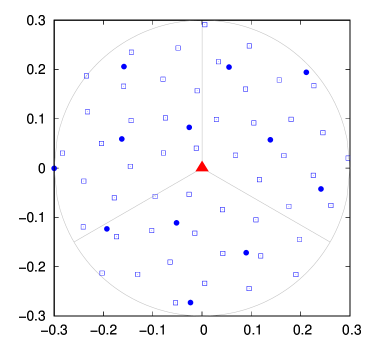
Figure 1: Base-station and receiver placement for $|B|=15$, $|K|=51$, and $R=0.3$ km. The three macrocells are represented by the single filled triangle at the center, the twelve picocells by filled circles, the $51$ receivers by empty squares.

All our computational results are based on using a genetic algorithm (GA) to solve the MINLP problem. We use brkgaAPI [10], an open-source, state-of-the-art framework for efficient GA implementations, and refer to the resulting GA as HetNetGA. The framework assumes all variables are continuous in the interval $(0,1]$, which is consistent with the problem’s $\alpha_{bk}$’s (since these can still be arbitrarily close to $0$) but not with the $a_{bk}$’s (since these must be either $0$ or $1$). In HetNetGA we circumvent this by substituting a proxy $a^{\prime}_{bk}\in(0,1]$ for each $a_{bk}$ and letting $a_{bk}=[a^{\prime}_{bk}>0.5]$. Moreover, all constraints must be implemented as penalties added to the objective function. We do this by keeping a count $v$ of constraint violations and re-expressing Eq. (14) as

$$P=P^{\mathrm{sf}}+P^{\mathrm{tx}}+vP^{\mathrm{viol}},$$ (21)

where $P^{\mathrm{viol}}$ is the penalty to be incurred per violation. We use

$$P^{\mathrm{viol}}=\sum_{b\in B}(P_{b}^{\mathrm{sf}}+P_{b}^{\mathrm{tx}}),$$ (22)

that is, the maximum possible value of $P$ in Eq. (14).

As a meta-heuristic, brkgaAPI can sometimes be nudged into better convergence to feasibility and subsequent optimization by tuning its behavior to problem-specific characteristics. We have found one such intervention to be particularly useful when designing HetNetGA. It consists in adding a further type of constraint to the MINLP problem in order to prevent the combined capacity available to receiver $k$ from surpassing $d_{k}$ by too wide a margin. For $\eta\in(0,1)$, the further constraint for each $k\in K$ is

$$\sum_{b\in B}a_{bk}(\alpha_{bk}-\eta)C_{bk}\leq d_{k},$$ (23)

so the capacity available to $k$, $\sum_{b\in B}a_{bk}\alpha_{bk}C_{bk}$, must not exceed $d_{k}$ by more than a fraction $\eta$ of that capacity’s maximum possible value, obtained by setting every $\alpha_{bk}$ to $1$. Violating this constraint does not alter the feasibility status of any given assignment of values to the problem’s variables but does contribute to the count $v$ affecting Eq. (21).

Tables 1 and 2 contain all parameter values used to obtain the results given in Section 6. Table 1 refers to the formulation of the MINLP problem, including the additional constraint in Eq. (23). The values for $L_{b}$ (for a center frequency of $2$ GHz and $d_{bk}$ in kilometers) and $\tau_{b}$ are from [11]. The values for $P_{b}^{\mathrm{sf}}$, $\phi_{b}^{\mathrm{sf}}$, $P_{b}^{\mathrm{tx}}$, and $\phi_{b}^{\mathrm{tx}}$ are loosely based on the discussion in [8]. By Eq. (13), we get $P_{b}=39.75$ W if $b$ is a macrocell, $P_{b}=1$ W if $b$ is a picocell. Likewise, by Eq. (22) we have $P^{\mathrm{viol}}=1\,500+(|B|-3)\,33$ W. The values for narrowband $N$ and gain $G$ imply a wideband $W=1.28$ GHz.

Table 2 refers to the inner operation of brkgaAPI and its use by HetNetGA: $p$ is the number of individuals (or chromosomes, in GA parlance) a population has, given in proportion to the number $n_{\mathrm{var}}=2|B||K|$ of variables (or alleles); $p_{\mathrm{e}}$ is the fraction of $p$ to be the elite set; $p_{\mathrm{m}}$ is the fraction of $p$ to be replaced by mutants; $\rho_{\mathrm{e}}$ is the probability of inheriting each allele from the elite parent; $n_{\mathrm{pop}}$ is the number of independent populations; and $n_{\mathrm{gen}}$ is the number of generations allowed to elapse before termination. Each individual is an assignment of values to the problem’s variables. Owing to the strictly positive value of $p_{\mathrm{e}}$, HetNetGA gives rise to an individual that minimizes $P$ in Eq. (21) globally with as high a probability as one wishes, provided the allotted $n_{\mathrm{gen}}$ is sufficiently large [12]. Of course, we have no efficient means of verifying whether this occurs for any given $n_{\mathrm{gen}}$, only of checking individuals for feasibility.

Table 1: Parameter values for the MINLP problem

Macrocells	Picocells	Decoding
$L_{b}=128.1$ dBm	$L_{b}=140.7$ dBm	$\gamma_{0}=1.174\times 10^{-20}$ J
$\tau_{b}=3.76$	$\tau_{b}=3.67$	$\beta=5$ dB
$P_{b}^{\mathrm{sf}}=235$ W	$P_{b}^{\mathrm{sf}}=28$ W	$N=10$ MHz
$\phi_{b}^{\mathrm{sf}}=0.85$	$\phi_{b}^{\mathrm{sf}}=0.5$	$G=128$
$P_{b}^{\mathrm{tx}}=265$ W	$P_{b}^{\mathrm{tx}}=5$ W	Eq. (23)
$\phi_{b}^{\mathrm{tx}}=0.85$	$\phi_{b}^{\mathrm{tx}}=0.8$	$\eta=0.005$

Table 2: Parameter values related to brkgaAPI

$p=10n_{\mathrm{var}}$	$p_{\mathrm{e}}=0.2$	$p_{\mathrm{m}}=0.1$
$\rho_{\mathrm{e}}=0.4$	$n_{\mathrm{pop}}=3$	$n_{\mathrm{gen}}=10\,000$

6 Results, conclusion, and outlook

All our results refer to the setting depicted in Figure 1. Within this setting we investigate five distinct scenarios, each forbidding certain base stations to ever be turned on. This can be enforced for any $b\in B$ by overriding Table 1 and setting $P_{b}^{\mathrm{tx}}=0$, thus leading to $\mathrm{SINR}_{bk}=0$ for every $k\in K$, and consequently to $a_{bk}=0$ (so $a_{b}=\rho_{b}=0$) whenever feasibility holds; cf. Eq. (17). We refer to the first scenario as 0m12p (no macrocells can ever be turned on, all picocells can), and similarly for the other four scenarios: 1m12p, 2m12p, 3m12p, and 3m0p. In relation to Figure 1, the shorthand 1m refers to the upper right sector, 2m to the two upper sectors. Notably, when no picocells are allowed to be turned on (scenario 3m0p), by Eq. (2) it follows that $\mathrm{SINR}_{bk}$ does not depend on the value of $G$ for any macrocell $b$ or any $k\in K$.

In what follows, every value we report for $P$, the total power consumed, is for feasible individuals and follows Eq. (14). Our results are summarized in Figures 2 and 3, where information related to the output of HetNetGA is given for all five scenarios and five values of demand $d_{k}$, the same for every $k\in K$. For the reader’s benefit, these figures are complemented by Figure 4, which relates our results to both the layout in Figure 1 and the statistics in Figure 2.

Figure 2: Best value of $P$, as per Eq. (14), obtained after $n_{\mathrm{gen}}$ generations for each scenario and each value of $d_{k}$. Averages refer to six independent runs of HetNetGA, with confidence intervals given at the $95\%$ level. Missing values indicate that feasibility was never attained for the corresponding combination of scenario and $d_{k}$ value.

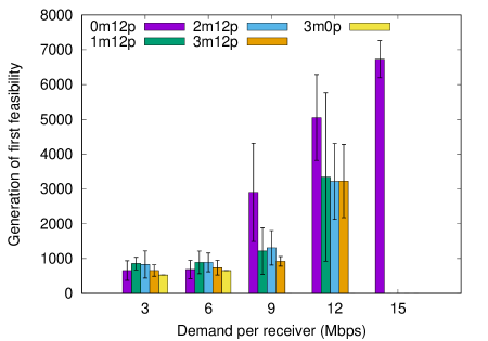
Figure 3: Generation of first feasibility in the context of Figure 2. Averages refer to the same six independent runs of HetNetGA, again with confidence intervals given at the $95\%$ level.

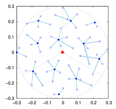
Figure 4: One of the solutions contributing to Figure 2 ($d_{k}=12$ Mbps, scenario 0m12p). Lines interconnecting receivers and picocells represent associations. Line thickness grows linearly with the corresponding $\alpha_{bk}$’s.

As expected, increasing $d_{k}$ increases total power consumption as well (Figure 2), and moreover makes feasibility ever harder to attain (Figure 3). Additionally, larger $\alpha_{bk}$’s tend to be necessary as base station $b$ and receiver $k$ are placed farther apart from each other (Figure 4). Unexpectedly, though, feasibility seems to become impossible for scenario 3m0p somewhere between $d_{k}=6$ and $9$ Mbps, and for the other scenarios involving one or more macrocells (1m12p, 2m12p, and 3m12p) somewhere between $d_{k}=12$ and $15$ Mbps (Figure 2). This rules out the use of macrocells for higher bit-rate demands, those for which picocells alone will not do (this holds already for $d_{k}=15.5$ Mbps; data not shown). Perhaps some sweet spot exists at which this happens, but locating it has proven elusive. As far as we have been able to observe, any assistance a macrocell might provide in meeting a certain bit-rate demand is offset by the interference it causes, and then the whole setting becomes energetically disadvantageous.

Naturally, the flip side of this conclusion is that HetNetGA, in spite of its properties of convergence to a global minimum, is after all the one to blame. Some support against this possibility is given in Figure 3, which shows how early feasibility is first attained during the $n_{\mathrm{gen}}$ generations. This happens ever later as $d_{k}$ increases, and also with confidence intervals much greater than those of Figure 2. The suggestion here is that, notwithstanding all the variation in the number of generations to hit first feasibility, by the $n_{\mathrm{gen}}$th generation the solutions HetNetGA outputs are approximately equivalent to one another. This hardly rules out the abovementioned sweet spot, but does make it hard enough to find to cast doubt on the practicality of looking for it.

Thus, insofar as the model outlined in Section 3 can be said to describe the system under study faithfully, a role is yet to be found for macrocells. Further research should concentrate on variations of this model, and also of its characteristics as summarized in Table 1, aiming to better delimit what can be expected of macrocells. HetNetGA, which inherently preserves the mathematical description of the associated MINLP problem, is expected to remain a useful tool.

Acknowledgments

This work was supported in part by Conselho Nacional de Desenvolvimento Científico e Tecnológico (CNPq), Coordenação de Aperfeiçoamento de Pessoal de Nível Superior (CAPES), and a BBP grant from Fundação Carlos Chagas Filho de Amparo à Pesquisa do Estado do Rio de Janeiro (FAPERJ).

References

- [1] Q. Kuang and W. Utschick. Energy management in heterogeneous networks with cell activation, user association, and interference coordination. IEEE Trans. Wireless Commun., 15:3868–3879, 2016.
- [2] B. Zhuang, D. Guo, and M. L. Honig. Energy-efficient cell activation, user association, and spectrum allocation in heterogeneous networks. IEEE J. Sel. Areas Commun., 34:823–831, 2016.
- [3] T. Zhou, N. Jiang, Z. Liu, and C. Li. Joint cell activation and selection for green communications in ultra-dense heterogeneous networks. IEEE Access, 6:1894–1904, 2018.
- [4] J. A. Ayala-Romero, J. J. Alcaraz, and J. Vales-Alonso. Energy saving and interference coordination in HetNets using dynamic programming and CEC. IEEE Access, 6:71110–71121, 2018.
- [5] J. A. Ayala-Romero, J. J. Alcaraz, A. Zanella, and M. Zorzi. Online learning for energy saving and interference coordination in HetNets. IEEE J. Sel. Areas Commun., 37:1374–1388, 2019.
- [6] Y. L. Lee, W. L. Tan, S. B. Y. Lau, T. C. Chuah, A. A. El-Saleh, and D. Qin. Joint cell activation and user association for backhaul load balancing in green HetNets. IEEE Wireless Commun. Lett., 9:1486–1490, 2020.
- [7] D. Tse and P. Viswanath. Fundamentals of Wireless Communication. Cambridge University Press, Cambridge, UK, 2005.
- [8] O. Arnold, F. Richter, G. Fettweis, and O. Blume. Power consumption modeling of different base station types in heterogeneous cellular networks. In Future Network & Mobile Summit Conf. Proc., 2010.
- [9] H. Vogel. A better way to construct the sunflower head. Math. Biosci., 44:179–189, 1979.
- [10] R. F. Toso and M. G. C. Resende. A C++ application programming interface for biased random-key genetic algorithms. Optim. Method. Softw., 30:81–93, 2015.
- [11] 3GPP. Further advancements for E-UTRA physical layer aspects. Technical Report 36.814 V9.0.0, 2010.
- [12] D. Greenhalgh and S. Marshall. Convergence criteria for genetic algorithms. SIAM J. Comput., 30:269–282, 2000.