NuPS: A Parameter Server for Machine Learning with Non-Uniform Parameter Access

Abstract.

Parameter servers (PSs) facilitate the implementation of distributed training for large machine learning tasks. In this paper, we argue that existing PSs are inefficient for tasks that exhibit non-uniform parameter access; their performance may even fall behind that of single node baselines. We identify two major sources of such non-uniform access: skew and sampling. Existing PSs are ill-suited for managing skew because they uniformly apply the same parameter management technique to all parameters. They are inefficient for sampling because the PS is oblivious to the associated randomized accesses and cannot exploit locality. To overcome these performance limitations, we introduce NuPS, a novel PS architecture that (i) integrates multiple management techniques and employs a suitable technique for each parameter and (ii) supports sampling directly via suitable sampling primitives and sampling schemes that allow for a controlled quality–efficiency trade-off. In our experimental study, NuPS outperformed existing PSs by up to one order of magnitude and provided up to linear scalability across multiple machine learning tasks.

1. Introduction

To keep up with increasing dataset sizes and model complexity, distributed training has become a necessity for large machine learning (ML) tasks. Distributed training enables (i) scaling to models and datasets that exceed the memory of a single machine by distributing them to the nodes of a compute cluster and (ii) faster training by performing distributed compute. Usually, each node accesses only its local part of the training data, but requires global read and write access to all model parameters. Parameter management is thus a key concern in distributed ML. Parameter servers (PS) ease distributed parameter management by providing primitives for reading and writing parameters, while transparently handling partitioning and synchronization across nodes (Smola and Narayanamurthy, 2010; Ahmed et al., 2012; Dean et al., 2012; Ho et al., 2013; Li et al., 2014). Many ML system stacks employ a PS as a core component, e.g., TensorFlow (Abadi et al., 2016), MXNet (Chen et al., 2015), PyTorch BigGraph (Lerer et al., 2019), STRADS (Kim et al., 2016), STRADS-AP (Kim et al., 2019), or Project Adam (Chilimbi et al., 2014), and there are many standalone PSs, e.g., Petuum (Ho et al., 2013), PS-Lite (Li et al., 2014), Angel (Jiang et al., 2017), FlexPS (Huang et al., 2018), Glint (Jagerman et al., 2017), PS2 (Zhang et al., 2019), Lapse (Renz-Wieland et al., 2020), and BytePS (Jiang et al., 2020).

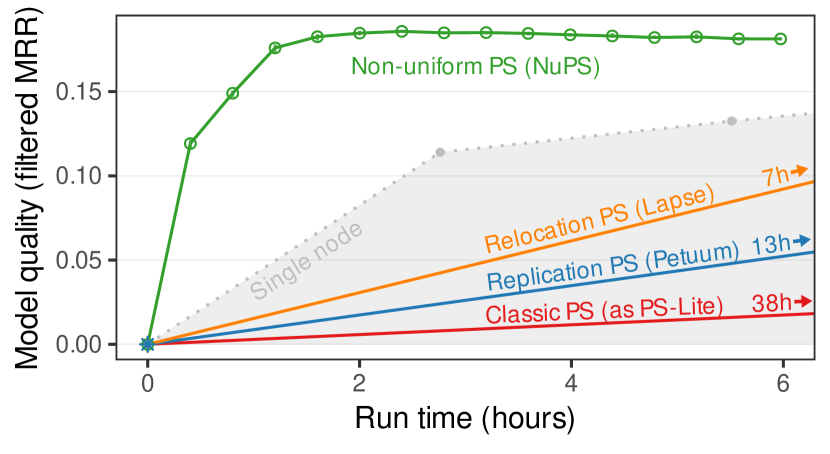
Figure 1. Parameter server (PS) performance for training large knowledge graph embeddings (ComplEx (Trouillon et al., 2016), dimension 500 on Wikidata5m data) on an 8-node cluster (8 worker threads per node). The performance of state-of-the-art PSs falls behind that of a single node (8 worker threads) due to communication overhead. NuPS improves performance by up to one order of magnitude. Details in Section 5.1.

As cluster nodes access parameters over the network, distributed training induces communication overhead. For some ML tasks, this overhead causes the performance of distributed implementations to even fall behind that of single node baselines (Renz-Wieland et al., 2020); Figure 1 depicts this exemplarily for a large knowledge graph embeddings task. We observe that a key cause for such poor performance can be non-uniform parameter access and focus on ML tasks where this is the case. We identify two main sources of non-uniformity: skew and sampling. First, in a workload that exhibits skew, a (typically small) subset of parameters is accessed frequently (e.g., up to $100\,000$ times per second), whereas a large part of the parameters is accessed rarely (e.g., only once every minute) (Meka et al., 2009; Cheng et al., 2016; Gonzalez et al., 2012; Faloutsos et al., 1999; Moreno-Sánchez et al., 2016; Clauset et al., 2009). The main reason for skew is that real-world datasets often have skewed frequency distributions (e.g., graphs (Cheng et al., 2016; Gonzalez et al., 2012; Faloutsos et al., 1999), texts (Moreno-Sánchez et al., 2016), and others (Clauset et al., 2009; Meka et al., 2009)), and many ML models associate specific parameters with specific data items (e.g., with the tokens in a text document or with the vertices of a graph) (Mikolov et al., 2013; Nickel et al., 2011; Koren et al., 2009)). The second source of non-uniformity is sampling: for a subset of parameter accesses, random sampling (rather than training data) determines which parameters are read and written (Mikolov et al., 2013; Ruffinelli et al., 2020; Liu et al., 2017; Rendle et al., 2009; Bamler and Mandt, 2020; Chechik et al., 2010; Schroff et al., 2015). One common reason for this access pattern is negative sampling (Mikolov et al., 2013; Bamler and Mandt, 2020; Ruffinelli et al., 2020; Grover and Leskovec, 2016), which, for example, is used to reduce the cost of many-class classification tasks or to mitigate an absence of negative training data (e.g., in recommender systems with only positive feedback or in knowledge graphs that contain only positive edges).

In this paper, we explore how to extend the scope of PSs to ML tasks that exhibit such non-uniform parameter access. To this end, we present NuPS, a novel non-uniform PS architecture. Figure 2 depicts an overview of this architecture. NuPS overcomes two key performance limitations of existing PSs. First, existing PSs are inefficient for managing skew because they employ one single management technique for all parameters. Using a single technique limits performance as none of the existing techniques is efficient for all access patterns. To overcome this limitation, NuPS introduces multi-technique parameter management, i.e., it integrates multiple parameter management techniques and chooses a suitable technique for each parameter. In particular, NuPS integrates both replication (Ho et al., 2013; Dai et al., 2015) and relocation (Renz-Wieland et al., 2020).

Figure 2. NuPS architecture. NuPS differs from existing PSs in two main ways: it introduces (i) multi-technique parameter management to handle skew and (ii) a sampling manager and API to handle sampling.

Second, existing PSs are inefficient for sampling because common parameter management techniques are ill-suited for randomly sampled access. To improve performance, applications can implement specialized sampling schemes manually, outside the PS (Lerer et al., 2019; Zheng et al., 2020; Ji et al., 2019; Stergiou et al., 2017), but this limits the efficiency of some schemes, potentially produces incorrect samples, and causes repeated implementation effort. NuPS overcomes this limitation by integrating sampling schemes directly into the PS. To do so, NuPS extends the PS API with a sampling primitive that allows applications to request samples from a specific sampling distribution (rather than accessing specific parameters directly). NuPS’s sampling manager transparently chooses one of several sampling schemes to reduce communication overhead for sampling, according to a conformity level. Conformity levels provide a controlled trade-off between efficiency and sample quality.

In our experimental evaluation, NuPS outperformed state-of-the-art PSs by up to one order of magnitude and provided up to linear scalability across multiple ML tasks. Figure 1 exemplarily shows its performance for the task of training knowledge graph embeddings.

In summary, our contributions are as follows: (i) we evaluate the suitability of existing PSs under skew (Section 3.1), (ii) we propose multi-technique parameter management to handle skew efficiently (Section 3.2), (iii) we develop a hierarchy of conformity levels (Section 4.1) and analyze properties of common sampling schemes (Section 4.2), (iv) we argue for and propose a PS API extension for sampling (Section 4.3) and present how NuPS implements several schemes behind this API (Section 4.4), and (v) we experimentally investigate how these changes affect PS performance (Section 5).

2. Non-Uniform Parameter Access

We study ML tasks that exhibit non-uniform parameter access. We identify two main sources of non-uniformity: skew (Section 2.1) and sampling (Section 2.2).

2.1. Skew

A workload exhibits skew non-uniformity when some parts of the model are accessed (much) more frequently than others. The main reason for this is that many real-world datasets have skewed frequency distributions (Meka et al., 2009; Cheng et al., 2016; Mohamed et al., 2020; Gonzalez et al., 2012; Faloutsos et al., 1999; Moreno-Sánchez et al., 2016; Clauset et al., 2009). For example, heavy skew is common in text corpora, because word frequencies are skewed (Moreno-Sánchez et al., 2016), and in graph data, because in- and out-degree distributions are skewed (Cheng et al., 2016; Mohamed et al., 2020; Gonzalez et al., 2012; Faloutsos et al., 1999). As many ML models associate specific parameters with specific data items (e.g, with words in a text or with the nodes of a graph) (Mikolov et al., 2013; Nickel et al., 2011; Koren et al., 2009; Grover and Leskovec, 2016), access to the parameters is heavily skewed, too: a small subset of hot spot parameters is accessed frequently, whereas the majority of parameters is accessed rarely. In the following, we will refer to the parameters that are not hot spots as long tail parameters.

We have measured the extent of skew for two real-world ML tasks: training knowledge graph embeddings and training word vectors. The left hand sides of Figures 3(a) and 3(b) show the number of reads per parameter over one epoch of these tasks, respectively. Access is heavily skewed: in the knowledge graph embeddings task, 18% of 12.9 trillion total reads go to only 0.02% of 4.8 billion parameters. In the word vectors task, 45% of 9 trillion total reads go to 0.17% of 1.9 billion parameters. Details on the tasks and datasets can be found in Section 5.1.

(a) Knowledge graph embeddings

(b) Word vectors

Figure 3. Number of accesses per parameter in one epoch. Parameters are sorted by decreasing total number of accesses. See Section 5.1 for details on tasks and experimental setup.

Note that skew is not always present in distributed training. For example, there is no skew in convolutional neural networks for image recognition (LeCun et al., 1989) because model access is dense, i.e., every update step writes to all parameters. In contrast, in common neural network models for natural language processing (Peters et al., 2018; Devlin et al., 2019; Howard and Ruder, 2018), access is partially dense, and partially sparse and skewed: access to the first (embedding) layer and sometimes the last (classification) layer is based on word or token frequency (and thus sparse and skewed), and access to other layers is dense. The share of parameters with frequency-based access depends on the model architecture, but can be high, e.g., around 90% in ELMo (Peters et al., 2018). In this paper, we investigate skew in shallow models, but conjecture that a non-uniform PS can also be beneficial for deeper models with partially skewed access.

2.2. Sampling

A workload exhibits sampling non-uniformity when, for a subset of parameter accesses, random sampling determines which parameters are read and written (Mikolov et al., 2013; Ruffinelli et al., 2020; Liu et al., 2017; Rendle et al., 2009; Rawat et al., 2021; Bamler and Mandt, 2020; Chechik et al., 2010; Schroff et al., 2015). I.e., the application randomly draws a parameter key from an application-specific sampling distribution over (all or a subset of) parameter keys. It then accesses the drawn parameter for training. We refer to such access as sampling access. In contrast, in direct access, the training data determines which parameters are accessed. Sampling access is common in many-class classification tasks, e.g., extreme classification (Bamler and Mandt, 2020), natural language processing (Mikolov et al., 2013), knowledge graph embeddings (Ruffinelli et al., 2020; Liu et al., 2017), graph representations (Grover and Leskovec, 2016; Yang et al., 2020), recommender systems (Rendle et al., 2009), and when triplet loss is used (Chechik et al., 2010; Schroff et al., 2015).

For example, knowledge graph embeddings and word vectors training tasks often use negative sampling to enable efficient training (Mikolov et al., 2013; Ruffinelli et al., 2020; Rawat et al., 2021). For each (positive) data point, a set of negative samples is drawn from a distribution. Each negative sample corresponds to a data item (e.g., a word) or a class. The corresponding parameters are subsequently accessed for training. For instance, the example knowledge graph embeddings task draws negative samples from a uniform distribution over all entities (Ruffinelli et al., 2020; Liu et al., 2017). The right hand side of Figure 3(a) shows the frequency distributions of direct and sampling accesses separately for this task. In our implementation (based on (Liu et al., 2017)) and with 200 negative samples for each subject–relation–object triple (100 negative samples for the subject and another 100 for the object), sampling accesses make up 31% of all accesses. In the word vectors task, negative samples correspond to words and the sampling distribution resembles the word frequencies in the training data (Mikolov et al., 2013), see Figure 3(b). In the plot for direct access, parameters that belong to the output layer of the task’s neural network are visually distinct from the other parameters. The reason for this is that the task draws samples only from the output layer, and parameters in the plot are sorted by total access frequency. In our implementation (based on (Mikolov et al., 2013)) and with 3 negative samples for each word–word pair, sampling accesses make up 56% of all parameter accesses in this task.

3. Multi-Technique Parameter Management

In this section, we analyze the suitability of existing PSs for ML tasks with skewed parameter access (Section 3.1) and argue that existing PSs are inefficient for managing skew because they employ one single management technique for all parameters. Based on this analysis, we propose multi-technique parameter management and discuss NuPS’s implementation (Section 3.2).

3.1. Analysis of Common Parameter Management Techniques

PSs (Smola and Narayanamurthy, 2010; Ahmed et al., 2012; Dean et al., 2012; Ho et al., 2013; Li et al., 2014; Jagerman et al., 2017; Zhang et al., 2019; Jiang et al., 2017; Huang et al., 2018; Renz-Wieland et al., 2020; Jiang et al., 2020) partition the model parameters across a set of servers. The PS provides pull and push primitives for global reads and writes to model parameters, respectively. In the data-parallel setting, the training data are partitioned to a set of workers. During training, each worker processes its local part of the training data (often multiple times) and continuously reads and updates model parameters. To coordinate parameter accesses across workers, each parameter is assigned a unique key. Many PSs physically co-locate the (logically distinct) servers and workers on the same nodes for efficiency, either in multiple processes per node (Li et al., 2014; Jagerman et al., 2017; Jiang et al., 2017) or within one process (Ho et al., 2013; Huang et al., 2018; Renz-Wieland et al., 2020).

Several techniques have been proposed for managing parameters among the cluster nodes in a PS. In the following, we discuss common techniques, briefly introducing each before analyzing its suitability for managing skew.

3.1.1. Classic PS

A classic PS allocates parameters to servers statically (e.g., via range partitioning of the parameter keys) and uses no replication (Smola and Narayanamurthy, 2010; Ahmed et al., 2012; Li et al., 2014). Thus precisely one server holds the current value of a parameter, and this server is used for all pull and push operations on this parameter. Classic PSs typically guarantee sequential consistency for operations on the same key (Renz-Wieland et al., 2020).

Analysis: The performance of a classic PS is limited for both hot spots and long tail parameters. The reason for this is that every parameter access uses the network: it incurs network latency for two messages (to and from the responsible server) and the parameter value is sent over the network once (from the server to the worker in a pull operation, in the other direction for a push operation). This network overhead is incurred for all parameters, i.e., hot spot and long tail ones. For hot spots, the overhead is incurred many times for a few parameters. In the long tail, the overhead is incurred a few times for each of many parameters.

3.1.2. Replication PS

A replication PS replicates parameters and tolerates some amount of staleness in the replicas (Ho et al., 2013; Huang et al., 2018; Jiang et al., 2017; Dai et al., 2015; Cui et al., 2014). Replication PSs provide weaker consistency guarantees, such as bounded staleness, and require applications to explicitly control staleness via special primitives (e.g., an “advance the clock” operation). There are two main protocols for creating and refreshing replicas in general-purpose PSs: SSP (Ho et al., 2013) creates a replica when a parameter is accessed and uses this replica until the staleness bound is reached (at which point the replica is terminated). ESSP (Dai et al., 2015) also creates a replica when a parameter is (first) accessed, but then maintains this replica throughout the entire training task (by repeatedly propagating updates). In both SSP and ESSP, nodes accumulate replica updates locally and propagate them to the responsible server at the subsequent “advance the clock” invocation. A subset of replication PSs specifically target deep learning workloads in which each node holds replicas of all parameters and replicas are updated synchronously after each step of mini-batch stochastic gradient descent (Zhang et al., 2017; Jayarajan et al., 2019; Hashemi et al., 2019; Jiang et al., 2020). In contrast to NuPS, these PSs focus on workloads in which (i) the model size does not exceed the memory capacity of a single node and (ii) synchronous replica updates are not prohibitively slow w.r.t. to computational cost; some further apply only to GPU-based training (Jiang et al., 2020).

Analysis: A replication PS is efficient for hot spots, but its benefit for the long tail is limited. Replication reduces network overhead (compared to a classic PS) if a replicated parameter value is used more than once and multiple updates can be sent to the PS in aggregated form. Replication further reduces access latency if a parameter value (within the acceptable staleness bound) is already locally available when a read operation is issued. Both is typically the case for hot spot parameters, even within relatively tight staleness bounds (because hot spot parameters are accessed frequently at each node). In contrast, long tail parameters are accessed infrequently. So it is unlikely that a long tail parameter is accessed more than once within reasonable staleness bounds (large staleness bounds commonly deteriorate model convergence (Ho et al., 2013)). For the same reason, SSP (which creates replicas on demand) does not reduce access latency for long tail parameters, because replicas are mostly “cold”. With its eager replica maintenance, ESSP ensures that replicas are always “warm” (after the first access to a parameter), but at the cost of significant over-communication: ESSP constantly updates all replicas, although replicas for long tail parameters are accessed rarely.

3.1.3. Relocation PS

A relocation PS asynchronously re-allocates parameters among nodes during run time so that access operations can be processed locally, without network communication (Renz-Wieland et al., 2020). Relocation PSs require applications to control allocation via special primitives (e.g., a “localize” operation). As classic PSs, relocation PSs can provide per-key sequential consistency (Renz-Wieland et al., 2020).

Analysis: A relocation PS is efficient for long tail parameters, but has limited benefit for hot spots. Relocation eliminates access latency if there is sufficient time to relocate a parameter between accesses at different nodes. It further reduces network overhead (compared to classic) if a parameter is accessed more than once between two relocations (which is common, most ML tasks at least read and write a parameter): a relocation takes three messages in Lapse (Renz-Wieland et al., 2020) (including the parameter value once), whereas each remote access in a classic PS sends two messages (including the parameter value once). There is typically sufficient time for relocating long tail parameters between accesses by different nodes, as they are accessed infrequently. Hot spot parameters, however, are frequently accessed at multiple nodes concurrently (Renz-Wieland et al., 2021). Thus, there is not sufficient time for relocations between accesses, such that access latency is not eliminated. Further, a relocation PS incurs higher network overhead than a classic PS if a parameter is relocated so frequently that only one operation is processed locally.

3.1.4. Summary

Individual management techniques are efficient for either hot spot or long tail parameters (or neither of the two), but none is efficient for both. Consequently, managing all parameters with the same technique limits the performance of PSs for ML tasks with skewed parameter access.

3.2. Parameter Management in NuPS

From the above discussion, it follows naturally to explore whether combining multiple management techniques is beneficial for PS performance. The idea of combining multiple management techniques has been studied in other (non-PS) distributed data management systems, such as general-purpose distributed databases (Dowdy and Foster, 1982; Wolfson and Jajodia, 1992; El Abbadi, 1991; Ciciani et al., 1990) and distributed graph processing systems (Low et al., 2012). These systems combine static allocation with replication, but do not consider relocation. To the best of our knowledge, integrating multiple management techniques in PSs has not been explored before.

NuPS integrates two management techniques: replication and relocation. First, to manage hot spot parameters efficiently, NuPS integrates a lightweight variant of eager replication (Dai et al., 2015). NuPS eagerly creates replicas for hot spot keys on all nodes and provides time-based staleness bounds. Basing the staleness bound on time rather than clocks alleviates the need for adding “advance the clock” operations to application code, but potentially complicates the analysis of convergence properties. We discuss these implications below. Second, to manage long tail parameters efficiently, NuPS integrates relocation. As Lapse (Renz-Wieland et al., 2020), NuPS asynchronously relocates these parameters before they are accessed. This guarantees per-key sequential consistency for long tail parameters. NuPS picks a technique for each key based on the key’s access pattern: if the key is accessed frequently, NuPS replicates the key; if there are few accesses, NuPS employs relocation (see Section 5.1). The choice of management technique is transparent to the application, i.e., the application accesses all parameters in the same way, via the push and pull primitives. Our experimental evaluation shows that the combination of replication and relocation can be highly beneficial. Integrating other techniques (e.g., highly tailored ones) may further improve performance, but is beyond the scope of this paper. NuPS does not integrate the classic technique as it is dominated by replication for hot spots and by relocation for the long tail.

Figure 4. Parameter management in NuPS. NuPS replicates hot spots and relocates long tail parameters. It accesses replicated and current local parameters via shared memory.

For efficiency, NuPS co-locates workers and servers in one process per node, and accesses replicas and locally allocated parameters via shared memory. Figure 4 depicts an overview. To access a key, a worker checks whether this key is managed by replication or relocation. If the key is managed by replication, the worker accesses the key via shared memory, without network communication. If the key is managed by relocation, the worker checks whether the key is currently allocated locally. If so, it accesses the key via shared memory. Otherwise, the worker accesses the parameter remotely, using the message protocol proposed in Lapse (Renz-Wieland et al., 2020): a request to the node that knows where the parameter is currently allocated, which then forwards the request to this node, which in turn processes the request and sends a response to the worker.

NuPS is designed to minimize the run time overhead of providing multiple management techniques. To do so, NuPS integrates the check for the management technique and the check for local allocation into one latch acquisition (i.e., a lock held for the duration of the API call). Further, NuPS can be reduced to a single-technique PS with no measurable run time overhead for providing more than one management technique: If replication is not used for any key, the replica synchronization background thread exits immediately, without sending any messages. If relocation is not used for any key, no messages are sent for relocation.

NuPS bases its staleness bounds on time rather than logical clocks because this makes the PS easier to use: time-based bounds alleviate the need for adding “advance the clock” operations to application code and for timing them appropriately. NuPS synchronizes the replicas periodically, using sparse all-reduce operations (i.e., only updated parameters are exchanged (Träff, 2010)). The synchronization is run by a background thread and uses the recursive doubling algorithm. However, time-based bounds potentially complicate the analysis of convergence properties. If only a bounded number of SGD steps can occur within one synchronization round, bounded staleness holds (as for clock-based staleness bounds) and the corresponding analysis carries over (Ho et al., 2013). However, if the number of SGD steps within one synchronization round cannot be bounded, convergence analyses for asynchronous SGD apply (Lian et al., 2015; Zhang et al., 2018). In our experiments, the effect of time-based bounds on performance was minimal because we used replication only for a small number of parameters and synchronized replicas frequently (see Section 5.6 and Section 5.7).

4. Sampling Management

Existing PSs provide no support for sampling. This means that applications manually sample keys and then access the corresponding parameters via direct access, which leads to significant communication overhead. To reduce this overhead, many applications implement a variety of sampling schemes (Lerer et al., 2019; Zheng et al., 2020; Ji et al., 2019; Stergiou et al., 2017). The key idea of such sampling schemes is that slightly (or sometimes rather significantly) deviating from the ideal of independent sampling from the desired target distribution might have only little or no effect on model quality, but can reduce communication overhead substantially (and consequently speed up model training). The lack of sampling support in PSs forces applications to implement such schemes in application code, outside the PS. This leads to repeated implementation effort and potentially produces incorrect samples. Further, this precludes schemes that require tight integration with parameter management.

In contrast to existing PSs, NuPS integrates sampling directly into the PS. In the following, we present the components of this integration. We first introduce a set of conformity levels that allow for a controlled trade-off between efficiency and sample quality (Section 4.1). We then analyze conformity and communication overhead of sampling schemes that are commonly used by applications (Section 4.2). Based on this analysis, we propose an API extension that enables sampling in PSs (Section 4.3) and discuss how NuPS implements several sampling schemes, within this API (Section 4.4).

4.1. Sampling Conformity Levels

Let $\pi$ be a target distribution over parameter keys. We assume that $\pi$ is specified by the application and remains fixed throughout run time. For example, in the word vectors training task of Section 2.2, the target distribution $\pi$ roughly corresponds to relative word frequencies (Mikolov et al., 2013); cf. Figure 3(b). When training knowledge graph embeddings, $\pi$ is often a uniform distribution over all entities (Ruffinelli et al., 2020); cf. Figure 3(a). Denote by $\mathcal{K}$ the set of parameter keys and by $\pi_{k}\geq 0$ the target probability for key $k\in\mathcal{K}$, where $\sum_{k=1}^{|K|}\pi_{k}=1$. Workers repeatedly draw one or more samples from the target distribution $\pi$. Denote by $X_{qi}\in\mathcal{K}$ a random variable for the $i$-th sample obtained at node $q$. We write $N_{q}$ for the number of samples drawn at node $q$ during the complete run time of some application. Set $\mathcal{X}_{q}=\{X_{q1},\ldots,X_{qN_{q}}\}$ and $\mathcal{X}=\bigcup_{q}\mathcal{X}_{q}$.

We propose a hierarchy of four sampling conformity levels to control the trade-off between sample quality and efficiency. From the top (L1) to the bottom (L4) of this hierarchy, sample quality decreases, and potential efficiency increases:

(L1) CONFORM.:

The sampling scheme produces mutually independent samples from the target distribution $\pi$. I.e.,

$$p(X_{qi}=k|\mathcal{S})=\pi_{k}$$

for all $q,i,k$ and $\mathcal{S}\subseteq\mathcal{X}\setminus\left\{\,X_{qi}\,\right\}$.

(L2) BOUNDED.:

The samples at each node have dependencies on past samples, but these dependencies are limited and samples at different nodes are independent. In more detail, given a dependency bound $B\in\mathbb{N}$, it holds

$$p(X_{qi}=k|\mathcal{S}_{q}^{-B},\mathcal{S}_{-q})=\pi_{k}$$

for all $q,i,k$, where $\mathcal{S}_{-q}\subseteq\mathcal{X}\setminus\mathcal{X}_{q}$ refers to samples at other nodes and $\mathcal{S}_{q}^{-B}\subseteq\{X_{q1},\ldots,X_{q(i-B-1)}\}$ refers to samples at node $q$ taken from all but the last $B$ samples taken so far. Note that first-order inclusion probabilities match the target probabilities—i.e., $p(X_{qi}=k)=\pi_{k}$—even though subsequent samples may be dependent. For example, a sampling scheme that internally draws independent samples from $\pi$ but uses each sample twice is BOUNDED with $B=1$.

(L3) LONG-TERM.:

The mean first-order inclusion probabilities match the target probabilities asymptotically at each node, i.e.,

(1) $$\lim_{N_{q}\to\infty}\frac{1}{N_{q}}\sum_{i=1}^{N_{q}}p(X_{qi}=k|X_{q1},\dots,X_{q(i-1)})=\pi_{k}$$

for all $q,k$. Note that this does not imply $p(X_{qi}=k)=\pi_{k}$. Also, arbitrary dependencies between samples within one or across multiple nodes are accepted as long as the asymptotic relative frequencies of the samples match the target. For example, a sequential sampling scheme that selects a random key order for the $|K|$ keys and then draws samples in a round-robin fashion satisfies LONG-TERM but not BOUNDED: each key is selected equally often in the long run, but the knowledge of the first $|K|$ samples allows to uniquely determine all future samples, so that no dependency bound can be established.

(L4) NON-CONFORM.:

No guarantees about the sampling probabilities or independence.

The levels are hierarchical in that L1 implies L2, and L2 implies L3. The first implication follows since we can set $\mathcal{S}=\mathcal{S}_{q}^{-B}\cup\mathcal{S}_{-q}$ for any choice of $\mathcal{S}_{q}^{-B}$ and $\mathcal{S}_{-q}$.

Proof (L2 implies L3).

Starting from some offset $1\leq o\leq B$, fix some node $q$ and consider the subset $\left\{\,X_{q(aB+o)}\,\right\}_{a\in\mathbb{N}}$ of every $B$-th sample on node $q$, starting from the $o$-th sample. Using the definition of BOUNDED, we obtain

$$\frac{1}{\lfloor(N_{q}-o)/B\rfloor}\sum_{a=1}^{\lfloor(N_{q}-o)/B\rfloor}p(X_{q(aB+o)}=k|X_{q1},\dots,X_{q(aB+o-B)})=\pi_{k}$$

for any choice of $N_{q}$, i.e., the long-term relative frequencies of every $B$-th sample match if we start at offset $o$. Since this holds for every offset $o$, we conclude that Eq. (1) holds and L2 implies L3. ∎

Note that we defined L3 via Eq. (1) rather than a simpler first-order probability condition such as $p(X_{qi}=k)=\pi_{k}$, because correct first-order conditions are not sufficient to ensure that a sampling scheme is useful in practice. For example, a sampling scheme that internally draws one independent sample $X$ from $\pi$, and then uses solely this sample throughout (i.e., $X_{qi}=X$ for all $q,i$) satisfies such a condition, but is clearly unsuitable in practice.

4.2. Analysis of Common Sampling Schemes

ML applications employ a variety of sampling schemes. In the following, we analyze schemes that are common in distributed training (Lerer et al., 2019; Zheng et al., 2020; Ji et al., 2019; Stergiou et al., 2017; Kochsiek and Gemulla, 2021) w.r.t. their effect on (i) communication overhead and (ii) sampling quality, i.e., into which conformity level they fall. Table 1 provides an overview of the latter.

Table 1. Conformity levels of common sampling schemes.

	L1	L2	L3
	CONFORM	BOUNDED	LONG-TERM
Independent sampling	✓	✓	✓
Sample reuse	$\times$	✓	✓
Local sampling	$\times$	$\times$	$\times$
Direct-access repurposing	$\times$	$\times$	$\times$

Independent sampling. Ideally, applications draw iid. samples from the target distribution and use each sample once. This scheme is CONFORM, but can lead to significant communication overhead: for each sample, the corresponding parameter values need to be transferred to the node and, after an update is computed, updates need to be propagated to other nodes.

Sample reuse. Sample reuse reduces communication overhead by using each sample multiple times (Ji et al., 2019; Zheng et al., 2020; Lerer et al., 2019; Broscheit et al., 2020). For example, knowledge graph embeddings training can use shared sampling, i.e., reuse negative samples for all positive examples in a mini-batch (Broscheit et al., 2020). Reusing a sample multiple times avoids the transfer of parameter values for another, fresh sample: using a sample $U$ times can reduce the communication overhead by a factor of $U$. We refer to this factor as the use frequency and to a sample reuse scheme that uses each sample $u$ times as U=u sample reuse. Sample reuse does not provide CONFORM since samples are not independent. However, it can provide BOUNDED. For example, if each fresh sample is sampled iid. from $\pi$ and then used exactly $U$ times, then the scheme is BOUNDED for all $B\geq U$. Moreover, in mini-batch negative sample reuse as in (Ji et al., 2019; Lerer et al., 2019; Broscheit et al., 2020), BOUNDED also holds. Here samples are reused only within one mini-batch of gradient descent so that the mini-batch size provides a bound on the sample dependency.

Local sampling. In many distributed ML architectures (Ho et al., 2013; Dai et al., 2015; Huang et al., 2018; Renz-Wieland et al., 2020), at each node, a distinct subset of the model parameters—the local partition—can be accessed without network communication. Local sampling restricts sampling accesses to this local partition (Zheng et al., 2020). This scheme eliminates network overhead for sampling accesses entirely. However, local sampling is NON-CONFORM as nodes see only samples from the local partition. Some implementations re-partition parameters periodically such that all nodes at least see all samples over time (Zheng et al., 2020). Careful re-partitioning might satisfy Eq. (1) for certain target distributions; e.g., if $\pi$ is uniform and parameters are allocated uniformly and at random. In general, however, local sampling cannot provide LONG-TERM. For example, consider any target distributions in which $\pi_{k}>{1}/{Q}$ for some $k$ (with $Q$ being the number of nodes). Local sampling cannot satisfy Eq. (1) for such a target since key $k$ is available for sampling at only one node at a time. This implies that there is at least one node at which the long-term frequency of $k$ is $\leq 1/Q$.

Direct-access repurposing. Another sampling scheme is to repurpose direct-access parameters, i.e., to use them as negative samples. For example, DGL-KE (Zheng et al., 2020) generates some of the samples by repurposing parameters that occur as positives in other data points of an SGD mini-batch. This requires no additional communication for sampling accesses, as the values for the direct access parameters are transferred to the node either way. In this scheme, the relative frequency of a seeing a key in a sample depends on the occurrence frequency of the key in the training data. As the training data occurrence distribution can be (and typically is (Broscheit et al., 2020; Mikolov et al., 2013)) different from the target distribution, this scheme is NON-CONFORM.

4.3. A Primitive for Sampling

It is impossible for PSs to integrate these sampling schemes within the push/pull API. The main problem is that sampling is done by application code: to conduct a sampling access, an ML application draws a sample of keys and accesses them via pull or push. For instance, this makes it impossible for the PS to restrict sampling to the local partition. Further, the PS cannot even distinguish between direct access (for which it cannot leverage sampling schemes) and sampling access (for which it can leverage sampling schemes).

To overcome these limitations, we propose to extend the PS API with a sampling primitive that allows applications to access a sample from a target distribution, under a specific sampling conformity level. The sampling manager in NuPS transparently chooses a sampling scheme that conforms with the chosen conformity level and applies the scheme for all sampling accesses. We propose one operation dist = register_distribution(π, L) to register a specific sampling distribution $\pi$ under a specific sampling conformity level $L$, and a combination of two operations to draw samples:

$$\mathtt{handle=} \mathtt{\ PrepareSample(dist,N)}$$

$$\mathtt{keys,values=} \mathtt{\ PullSample(handle[,n_{j}])}$$

The argument $N$ is the number of desired samples. PrepareSample is intended to return instantaneously (and run preparatory work in the background), PullSample blocks if called synchronously. After PullSample returns, the corresponding keys are stored in keys and corresponding values are copied to values. Applications can call PullSample once to obtain all $N$ samples at once or multiple times to obtain the $N$ samples in smaller portions (by passing $n_{0},n_{1},...<N$ to multiple invocations of PullSample such that $\sum n_{j}=N$). Such partial pulls give the PS more flexibility, and, thus, may result in better performance.

Figure 5. Sampling scheme implementations in NuPS.

This extension provides sufficient flexibility for implementing a wide range of sampling schemes, as we describe in the following Section 4.4. The extension derives its flexibility from three key design choices. First, the extension transfers sampling from the application to the PS. Second, the extension provides the PS with a hook for doing preparatory work, such as pre-fetching parameter values, modifying partitions, or coordinating among nodes. Third, the extension does not force final decisions (e.g., about the sampled keys) before PullSample returns.

4.4. The Sampling Manager in NuPS

The sampling manager is responsible for generating samples and managing the corresponding parameters. The sampling manager of NuPS currently supports four sampling schemes behind the sampling API. Figure 5 provides an overview. Schemes implement PrepareSample and PullSample, and optionally a background thread. From the four implemented schemes, the sampling manager picks a scheme that is suitable for the specified conformity level. We now discuss the schemes in turn.

Independent sampling (CONFORM). In this scheme, NuPS samples iid. from the target distribution and localizes the corresponding parameters in PrepareSample (such that they can be accessed locally when PullSample is called). In PullSample, NuPS accesses the parameters remotely if they have been relocated to another node in-between PrepareSample and PullSample (this can happen because other nodes can independently work on the same parameters). This approach is CONFORM because each worker samples iid. from $\pi$.

Table 2. ML tasks, models, datasets, and share of direct and sampling access.

Task	Model parameters				Data			Parameter access
	Model	Keys	Values	Size	Dataset	Data points	Size	Direct	Sampling
Knowledge graph embeddings	ComplEx, dim. $500$	$4.8\text{\,}\mathrm{M}$	$4.8\text{\,}\mathrm{B}$	$35.9\text{\,}\mathrm{G}\mathrm{B}$	Wikidata5M	$21\text{\,}\mathrm{M}$	$317\text{\,}\mathrm{M}\mathrm{B}$	69%	31%
Word vectors	Word2Vec, dim. $1000$	$1.9\text{\,}\mathrm{M}$	$1.9\text{\,}\mathrm{B}$	$7.0\text{\,}\mathrm{G}\mathrm{B}$	1b word benchmark	$375\text{\,}\mathrm{M}$	$3\text{\,}\mathrm{G}\mathrm{B}$	44%	56%
Matrix factorization	Latent Factors, rank 1000	$11.0\text{\,}\mathrm{M}$	$11\text{\,}\mathrm{B}$	$82.0\text{\,}\mathrm{G}\mathrm{B}$	$10\text{m}\times 1\text{m}$ matrix, zipf 1.1	$1000\text{\,}\mathrm{M}$	$31\text{\,}\mathrm{G}\mathrm{B}$	100%	0%

Sample reuse (BOUNDED). NuPS implements a sample reuse scheme that reuses pools of keys. The pooling increases the temporal distance between the reused samples and thereby increases randomness. For a given pool size $G$ and use frequency $U$, NuPS repeatedly samples $G$ keys iid. from $\pi$ to form a sample pool and produces samples by traversing the sample pool $U$ times, each time in a random order. For example, consider $U=2$ and suppose that the iid. draws produce keys $k_{1}$, $k_{2}$, and $k_{3}$, respectively. With $G=1$, we obtain sample sequence $k_{1}k_{1}k_{2}k_{2}k_{3}k_{3}$. With $G=3$, a sequence such as $k_{1}k_{2}k_{3}k_{2}k_{1}k_{3}$ is possible. The pools are prepared by a background thread. When the background thread generates a new pool, it localizes the corresponding parameters. NuPS localizes the parameters again in PrepareSample if they have been relocated to another node since pool preparation. In PullSample, NuPS accesses the parameters remotely if necessary. This sample reuse scheme is BOUNDED because samples are drawn iid. from the target distribution $\pi$, inter-sample dependency is bounded by $U\cdot G$, and $U$ is identical for all samples.

The background thread determines automatically when to prepare a new pool. Adding a new pool takes time and (for good performance) the localization should be finished when PullSample is called. This time depends on the ML task, the used hardware, and the system configuration. To estimate this time, we use a heuristic. In particular, the background thread keeps track of the duration of previous pool relocations. If the number of prepared, but unused samples is less than double of the current estimated relocation time, the preparation of another pool is triggered.

Sample reuse with postponing (LONG-TERM). NuPS additionally implements sample reuse with sample postponing. This is identical to the described sample reuse scheme, but adds sample postponing: if sample $i$ cannot be accessed locally in PullSample, NuPS re-localizes the corresponding parameters, postpones sample $i$ for later use, and uses sample $i+1$ instead. To achieve LONG-TERM, it is crucial that, at some point, samples are used (and not re-postponed indefinitely). Thus, NuPS postpones only within the $N$ samples of one invocation of PrepareSample (in other words, only within the samples of one handle). I.e., when NuPS finds a non-local sample (in PullSample), it moves the sample to the end of the $N$ samples of this handle. NuPS postpones each sample maximally once. When it reaches samples that it has already postponed once (towards the end of the $N$ samples), it accesses them remotely if necessary. This implementation of postponing reduces communication overhead only if the samples of one handle are pulled in groups smaller than $N$ and there is some time between these partial pulls for the parameter relocation. Assuming that $N$ is bounded from above, it provides LONG-TERM. It does not provide BOUNDED because sampling probabilities depend on the current allocation of a key (i.e., keys can be postponed to a later sample if they are not local).

Local sampling (NON-CONFORM). NuPS implements local sampling without active re-partitioning. Instead, NuPS relies on the application to relocate parameters: in a relocation PS, the local partition usually changes constantly, as workers relocate the parameters that they work with (in direct access). The effect of this local sampling variant heavily depends on the relocations of the application. Generally, this approach cannot give any guarantees, as, for example, an application might not relocate parameters at all. Thus, it generally falls into the NON-CONFORM level. In an ideal setting, however, this approach could provide LONG-TERM. For example, this can be the case if an application partitions its training data randomly and continuously relocates all parameters (such that a parameter is equally likely to be on all nodes) and samples uniformly (such that $\pi_{k}\ll\frac{1}{Q}$ for all $k$). To make local sampling efficient, NuPS employs a fast sampling implementation that does not sample independently.

5. Experiments

We conducted an experimental study to investigate whether and to what extent a non-uniform PS is beneficial for PS performance. Source code, datasets, and information for reproducibility are available online.

In our study, we compared the performance of NuPS to several state-of-the-art PSs on three large-scale ML tasks (Section 5.2). Further, we conducted an ablation study (Section 5.3), investigated scalability (Section 5.4), evaluated different sampling schemes (Section 5.5), and explored specific components of NuPS (Sections 5.6 and 5.7). Our major insights are: (i) NuPS was more than an order of magnitude faster than existing PSs. (ii) NuPS achieved best performance when it replicated a small fraction of the model parameters, and relocated all other parameters. (iii) Both sample reuse and local sampling significantly reduced communication overhead for sampling access. We conclude that a non-uniform PS is key for high performance in ML tasks with non-uniform parameter access.

5.1. Experimental Setup

We considered three popular ML tasks that require long training: knowledge graph embeddings, word vectors, and matrix factorization. These tasks are representatives for shallow models that exhibit sparse and skewed access. The tasks differ in multiple ways, including the number of parameters, parameter access distributions, sampling distribution, and frequency of sampling accesses. Table 2 provides a summary. In the following, we briefly discuss each task.

Knowledge graph embeddings. Knowledge graph embedding (KGE) models learn algebraic representations of the entities and relations in a knowledge graph. For example, these representations have been applied successfully to infer missing links in knowledge graphs (Nickel et al., 2016). This task, based on (Liu et al., 2017), trains ComplEx (Trouillon et al., 2016) (one of the most popular KGE models) embeddings using SGD with AdaGrad (Duchi et al., 2011) and negative sampling (Ruffinelli et al., 2020; Liu et al., 2017). Negative sampling creates sampling access in this task: to generate negative samples, both the subject and the object entity of a positive triple are perturbed $n_{\operatorname{neg}}$ times, by drawing random entities from a uniform distribution over all entities (we used a common setting of $n_{\operatorname{neg}}=100$ (Ruffinelli et al., 2020)). We used the Wikidata5M dataset (Wang et al., 2019), a real-world knowledge graph with $4\,818\,679$ entities and $828$ relations, and a common embedding size of $500$ (Ruffinelli et al., 2020). We partitioned the subject–relation–object triples of the dataset to the nodes randomly, as done in (Kochsiek and Gemulla, 2021). We used LibKGE (Broscheit et al., 2020) (commit 3146885) to evaluate models and report the mean reciprocal rank (filtered) (MRRF) as metric for model quality.

Word vectors. Word vectors (WV) are a language modeling technique in natural language processing: each word of a vocabulary is mapped to a vector of real numbers (Mikolov et al., 2013; Pennington et al., 2014; Peters et al., 2018). These vectors are useful as input for many natural language processing tasks, for example, syntactic parsing (Socher et al., 2013) or question answering (Liu et al., 2018). This task, based on (Mikolov et al., 2013), uses SGD and negative sampling to train the skip-gram Word2Vec (Mikolov et al., 2013) model (dimension 1000) on the One Billion Word Benchmark (Chelba et al., 2013) dataset (with stop words of the Gensim (Řehůřek and Sojka, 2010) stop word list removed). The negative sampling creates sampling accesses: in this task, for each word pair, 3 negative samples are drawn from a distribution that is based on word frequencies (see Section 2.2). We used common model parameters (Mikolov et al., 2013) for window size (5), minimum count (1), and frequent word subsampling (0.01). We measured model accuracy using a common analogical reasoning task of $19\,544$ semantic and syntactic questions (Mikolov et al., 2013).

Matrix factorization. Low-rank matrix factorization (MF) is a common tool for analyzing and modeling dyadic data, e.g., in collaborative filtering for recommender systems (Koren et al., 2009). This task, based on (Teflioudi et al., 2012), uses SGD to factorize a synthetic, zipf-1.1 distributed $10\text{m}\times 1\text{m}$ dataset with 1b revealed cells, modeled after the Netflix Prize dataset. Data points were partitioned to nodes by row and to workers within a node by column. Each worker visited its data points by column (to create locality in column parameter accesses), with random order of columns and of data points within a column. There is no sampling access in this task. We report the root mean squared error (RMSE) on the test set as metric for model quality.

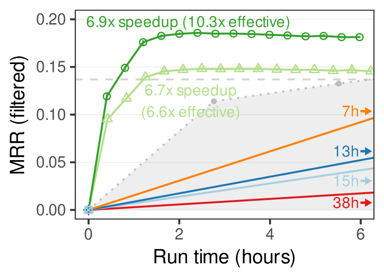
(a) KGE (quality over time)

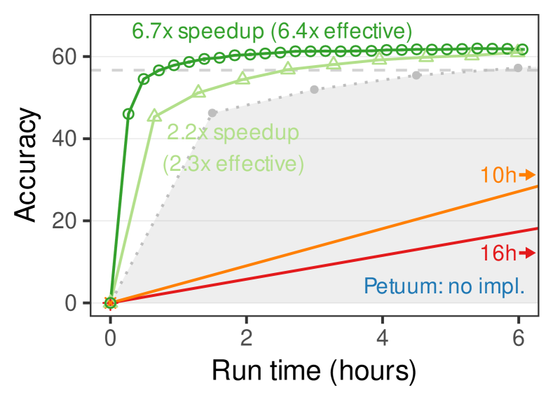
(b) WV (quality over time)

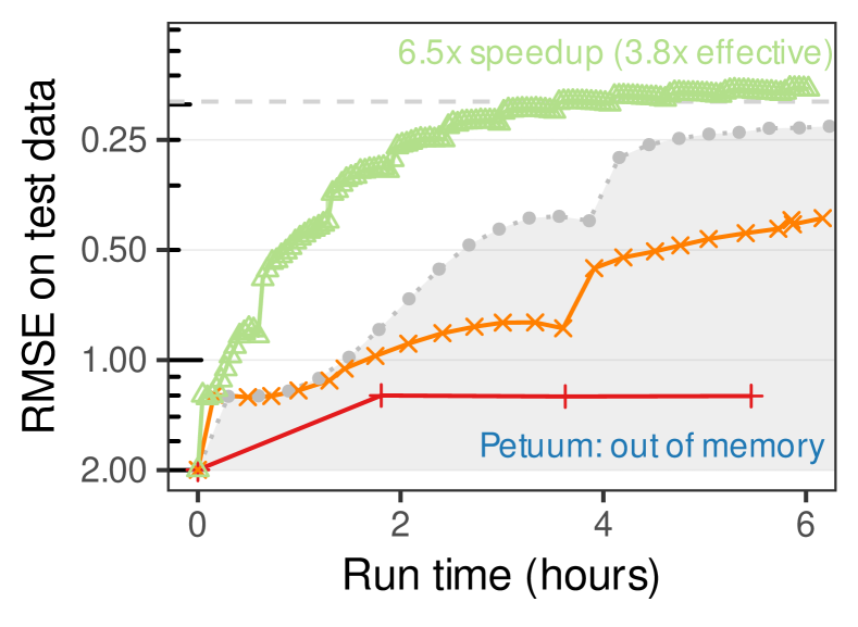
(c) MF (quality over time)

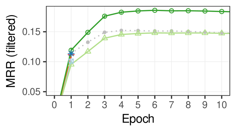
(d) KGE (quality over epoch)

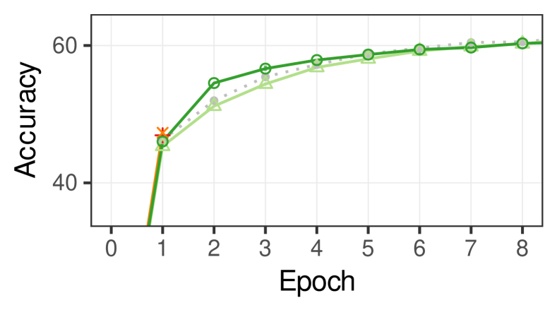
(e) WV (quality over epoch)

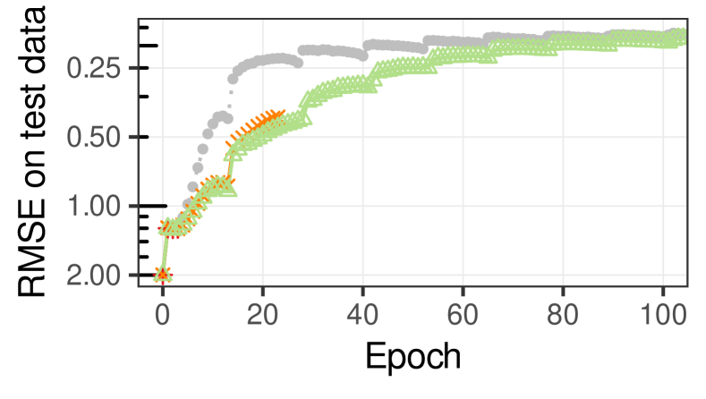
(f) MF (quality over epoch)

Figure 6. End-to-end performance of different PSs on 8 nodes. NuPS outperformed Petuum (a state-of-the-art replication PS) and Lapse (a state-of-the-art replication PS) by up to one order of magnitude and provided up to linear scalability over the single node. The gray shaded area indicates performance that is dominated by the single node. Error bars depict minimum and maximum measurements for run time and model quality (but are often not visible due to low variance). The dashed gray line depicts the model quality threshold at which effective speedups are computed (90% of the best observed single-node quality).

Baselines. We compared performance to a classic PS, to Petuum (a state-of-the-art replication PS), to Lapse (a state-of-the-art relocation PS), and to a single node implementation. As classic PS, we used Lapse with relocation disabled, which, according to (Renz-Wieland et al., 2020), provides performance similar to PS-Lite. We ran both the SSP and ESSP protocols of Petuum (Xing et al., 2015), with different staleness thresholds. Petuum does not provide KGE or WV implementations. Thus, we implemented the KGE task described above in Petuum. We used version 1.1 of Petuum. We did not implement specific sampling schemes in application code, i.e., applications draw independent samples and access them via direct access. We used a shared memory implementation with 8 worker threads as single node baseline.

Implementation and cluster. We implemented NuPS in C++, using ZeroMQ and Protocol Buffers for communication, based on PS-Lite (Li et al., 2014). We used a local cluster of up to 16 Lenovo ThinkSystem SR630 computers, running Ubuntu Linux 20.04, connected with 100 Gbit Infiniband. Each node was equipped with two Intel Xeon Silver 4216 16-core CPUs, 512 GB of main memory, and one 2 TB D3-S4610 Intel SSD. We compiled code with g++ 9.3.0, except for Petuum, which we compiled with g++ 7.5.0, as the compilation with g++ 9.3.0 failed. Unless specified otherwise, we used 8 nodes and 8 worker threads per node. In Lapse and NuPS, we additionally used 1 server and 3 ZeroMQ I/O threads per node. In Petuum, we used 4 communication channels per node. To prevent exploding gradients, we used gradient norm clipping as suggested in (Pascanu et al., 2013) for replicated parameters in the WV and MF tasks (clipping updates that exceed the average norm by more than 2x). In the KGE task, the use of AdaGrad prevented exploding gradients. For each task, we tuned hyperparameters on the single node and used the best found hyperparameter setting in all systems and variants.

NuPS. We ran NuPS in two configurations: (i) a generally applicable untuned configuration that requires no task-specific tuning and (ii) a task-specific tuned configuration. The untuned configuration employs a heuristic to decide the management technique for each parameter: it replicates a parameter if its access frequency exceeds $100$ times the mean access frequency. This heuristic is computed from dataset frequency statistics. The untuned configuration further employs sample reuse without postponing (BOUNDED) with a use frequency of U=16. To indicate the performance potential of task-specific insights, we included a tuned configuration by informing our configuration choices with the results of our detail experiments in Sections 5.5 and 5.6. The tuned configuration for KGE replicates the 900 most frequently accessed keys (the same as the untuned setting), but uses local sampling (NON-CONFORM). The tuned configuration for WV replicates the $209\text{\,}\mathrm{k}$ most frequently accessed keys (64x more keys than the untuned configuration), and employs local sampling (NON-CONFORM). For MF, the untuned configuration seemed to be near-optimal, such that we did not add a separate tuned configuration. Unless mentioned otherwise, we used the settings of the untuned configuration and a replica staleness threshold of $40\text{\,}\mathrm{m}\mathrm{s}$ in all experiments. Throughout all experiments, we used a pool size of 250 in the sample reuse scheme.

Measures. Unless noted otherwise, we ran all variants with a fixed $6\text{\,}\mathrm{h}$ time budget. We measured model quality over time and over epochs within this time budget (using the quality metrics described above). We conducted 3 independent runs of each experiment, each starting from a distinct randomly initialized model, and report the mean. We depict error bars for model quality and run time; they present the minimum and maximum measurements. In some experiments, error bars are not clearly visible because of small variance. Gray dotted lines indicate the performance of the single node baseline. Gray shading indicates performance that is dominated by the single node baseline. We report two types of speedups: (i) raw speedup depicts the speedup in epoch run time, without considering model quality; (ii) effective speedup is calculated from the time that each variant took to reach 90% of the best model quality that the single node baseline achieved. Unless specified otherwise, we report effective speedups.

5.2. Overall Performance

We investigated the overall effect of a non-uniform PS on PS performance. To do so, we compared the performance of NuPS to existing PSs and to the single node baseline. We ran each variant for the fixed time budget and measured model quality over this time. Figures 6(a), 6(b), and 6(c) show model quality over time, Figures 6(d), 6(e), and 6(f) show model quality over epoch. In summary, NuPS was 31–36x faster than a state-of-the-art replication PS (Petuum), 6–46x faster than a state-of-the-art relocation PS (Lapse), and 2.3–10.3x faster than the single node baseline.

The classic PS was inefficient (with epochs over 7x slower than the single node) because it accesses parameters over the network, which induced significant access latency. Lapse was faster than Classic, but still slower than the single node, because Lapse relocates all parameters, including hot spots. Hot spot parameters, however, are frequently accessed by multiple nodes simultaneously (Renz-Wieland et al., 2021), such that some of these nodes had to wait for the relocation to finish or access the parameter remotely, which induced access latency. The per-epoch model quality of Classic and Lapse was indistinguishable from the single node in KGE and WV, as these systems provide sequential consistency for all parameters and employ no specialized sampling schemes. In MF, all distributed variants provided lower per-epoch quality than the single node, an effect that has been observed before (Makari et al., 2015). The step pattern that is visible in MF training stems from the bold driver heuristic (Battiti, 1989) that the MF implementation (Makari et al., 2015) that we adapted uses to tune the learning rate.

For KGE, we ran Petuum SSP and ESSP with staleness thresholds 1, 10, 100, 200, or 1000, and tried different frequencies for advancing the clock. None of the configurations completed the first epoch within the time budget of 6 hours. We observed the best performance for ESSP with staleness 10, which finished the first epoch after 13h with a model quality (MRRF) of 0.11. The best SSP run (staleness 200) finished the first epoch after 15h with a model quality of 0.10. The reasons for this performance are that Petuum is inefficient for long tail parameters (as discussed in Section 3.1) and that Petuum’s replica approach is inefficient for sampling because sampling access provides no locality: SSP replicas are mostly cold, ESSP over-communicates. Petuum’s MF implementation ran out of memory, because it stores the training matrix in dense format.

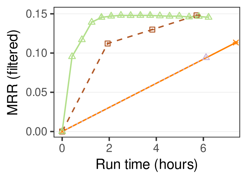
(a) Ablation, KGE

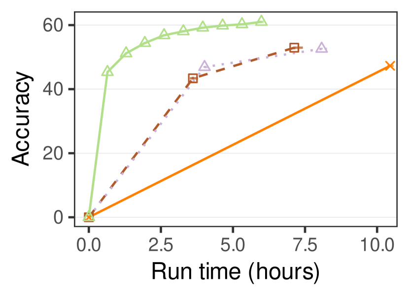
(b) Ablation, WV

Figure 7. Ablation. Both (i) combining replication and relocation and (ii) integrating specialized sampling access management techniques improved performance individually, and it was beneficial to combine the two.

The untuned NuPS configuration outperformed existing PSs across all three tasks. For KGE and MF, it was also clearly faster than the single node, with up to 6.7x effective speedups over the single node and minimal negative effect on (per-epoch) model quality. For WV, however, it barely outperformed the single node (but still outperformed existing PSs). In contrast, the tuned configuration provided 4.6–10.3x effective speedups over the single node across all three tasks. For KGE, the tuned configuration of NuPS provided better per-epoch convergence than the single node. This was an effect of local sampling; see Section 5.5 for more details.

5.3. Ablation

NuPS introduces two novel features compared to existing PSs: (i) multi-technique parameter management and (ii) the integration of sampling into the PS. To investigate individual effects, we enabled each feature individually and measured model quality within the time budget. Figure 7 shows the results. We omit MF because there is no sampling access in MF, such that the entire performance improvement stems from multi-technique parameter management (which is visible in Figure 6(c)). We found that both multi-technique parameter management and sampling integration can be beneficial individually, and the individual benefits compounded when both were combined.

We compared the performance of four variants: (i) Lapse, a relocation PS without sampling integration; (ii) Relocation + Replication, a PS with multi-technique parameter management but without sampling integration; (iii) Relocation + Sampling, a relocation-only PS with sampling integration; (iv) NuPS, a multi-technique PS with sampling integration. Going from a single-technique relocation PS to a multi-technique PS made an epoch 67–73% faster with only small effect on model quality. Adding sampling support to the relocation PS made an epoch 17–62% faster, with a small negative effect on model quality. The combination of both made an epoch 94% faster, with a small negative effect on per-epoch model quality.

5.4. Scalability

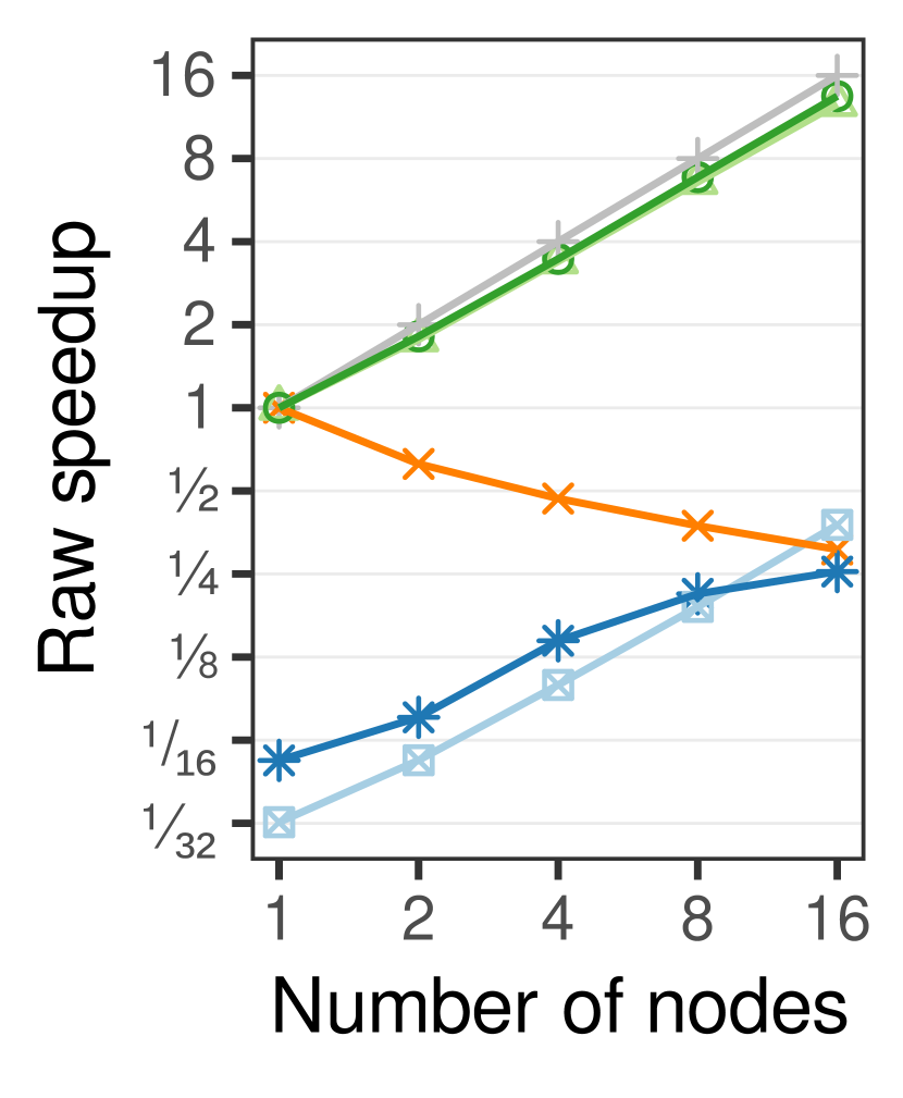
(a) KGE

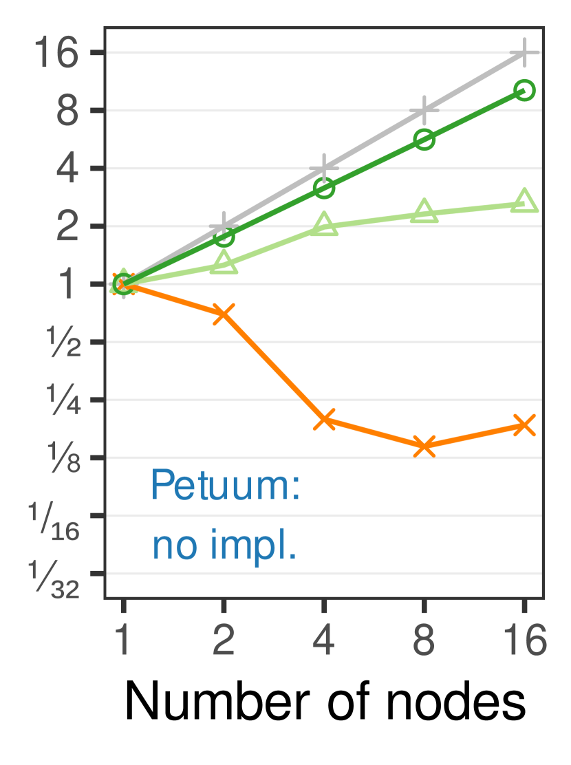
(b) WV

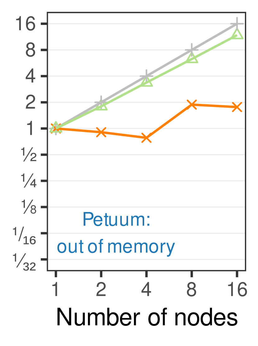
(c) MF

Figure 8. Raw scalability (logarithmic axes). The y-axis depicts raw speedup, i.e., speedup w.r.t. epoch run time over the shared-memory single-node baseline. NuPS scaled more efficiently than other PSs, with up to near-linear speedups.

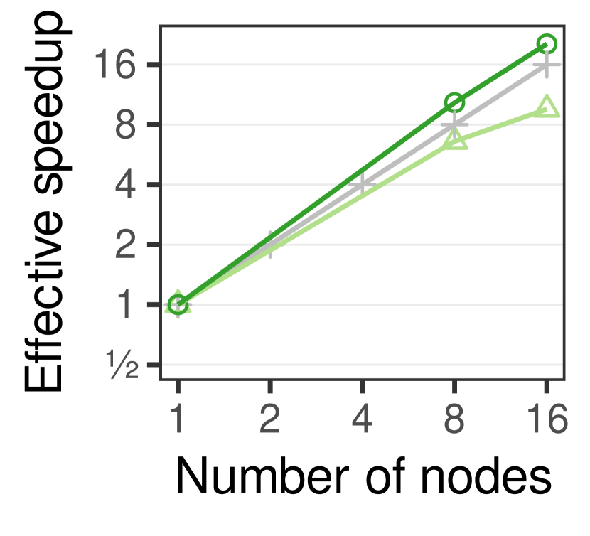
(a) KGE

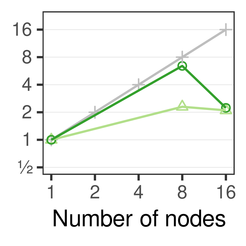
(b) WV

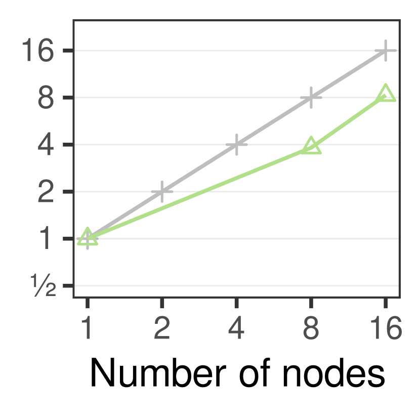
(c) MF

Figure 9. Effective scalability (logarithmic axes). The y-axis depicts effective speedup, i.e., speedup w.r.t. reaching 90% of the best model quality observed on a single node.

To investigate scalability, we ran Lapse, the best Petuum SSP and ESSP configurations, and NuPS for one epoch on 1, 2, 4, 8, and 16 nodes and calculated the raw speedup. Figure 8 depicts the results. Further, we ran convergence experiments on 16 nodes for those systems that reached the 90% model quality threshold on 8 nodes. Figure 9 depicts the effective speedup for these systems. Overall, NuPS scaled more efficiently than other PSs, with up to near-linear raw and up to superlinear effective speedups.

We first discuss raw scalability, i.e., the speedup w.r.t. epoch run time (Figure 8). On a single node, NuPS and Lapse were faster than Petuum because NuPS and Lapse access local parameters via shared memory, whereas Petuum sends intra-process messages to do so. Lapse provided poor scalability because the more nodes are used, the higher the chance that multiple nodes access a parameter at the same time and, thus, that they have to wait for a relocation to finish or to access parameters remotely. Neither Petuum ESSP nor SSP outperformed the shared-memory single-node baseline, even on 16 nodes. ESSP scaled poorly even when compared to its own (inefficient) run time on a single node (4.8x faster on 16 nodes) because its eager replication protocol over-communicates: after a short warm-up period, each node holds a replica of the full model. The more nodes, the more replicas had to be synchronized, such that replica synchronization became a bottleneck. The lazy replication protocol of SSP scaled better than ESSP compared to its own (inefficient) run time on a single node (12x faster on 16 nodes), but its overall performance was poor because its replicas were cold most of the time (and thus required synchronous replica refreshes).

NuPS scaled more efficiently than existing PSs because it (i) limits the bottleneck of eager replication by replicating only a small subset of hot spot parameters, (ii) prevents the majority of relocation conflicts by employing relocation only for long tail parameters, and (iii) employs sampling schemes to reduce sampling communication overhead. With 16 nodes, it provided up to 13.4x raw speedups over the shared memory single node. NuPS further provided up to 20x effective speedups for KGE and 8x for MF (see Figure 9). For WV, although the raw speedup on 16 nodes was 10.2x, the effective speedup was only 2.2x. The reason for this is that we used the hyperparameter configuration that worked best on the single node throughout all experiments. With other hyperparameters, we observed better effective speedups for WV.

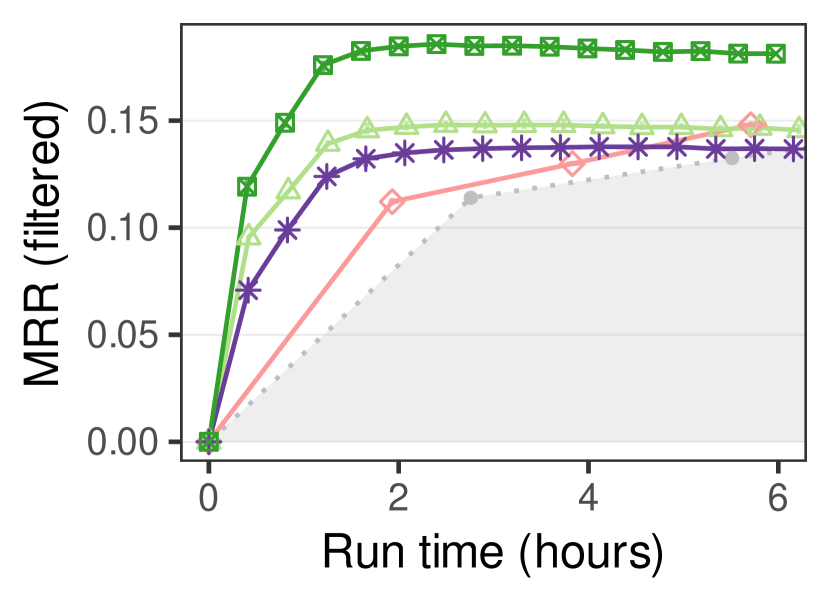
(a) KGE (quality over time)

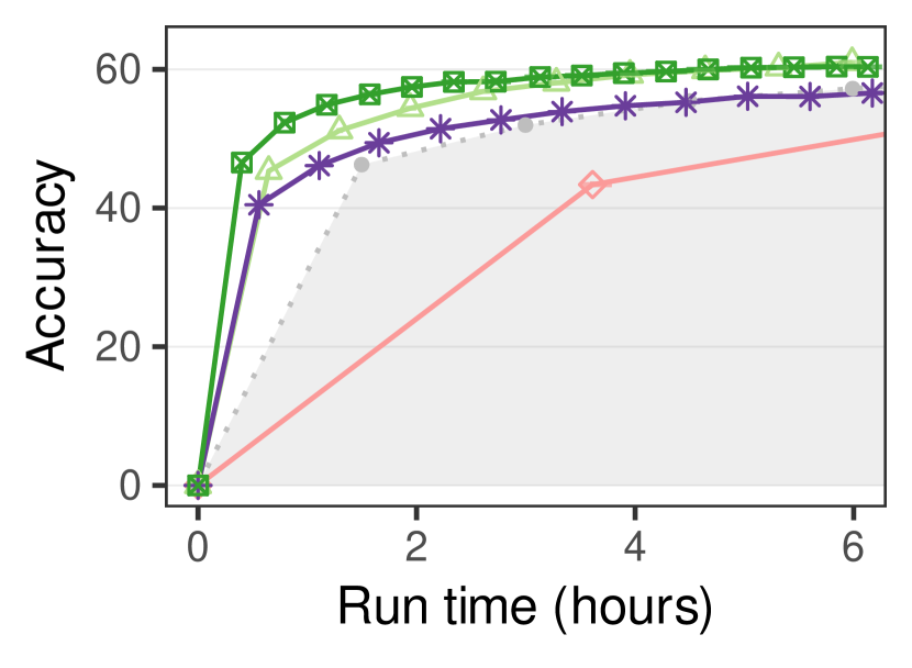
(b) WV (quality over time)

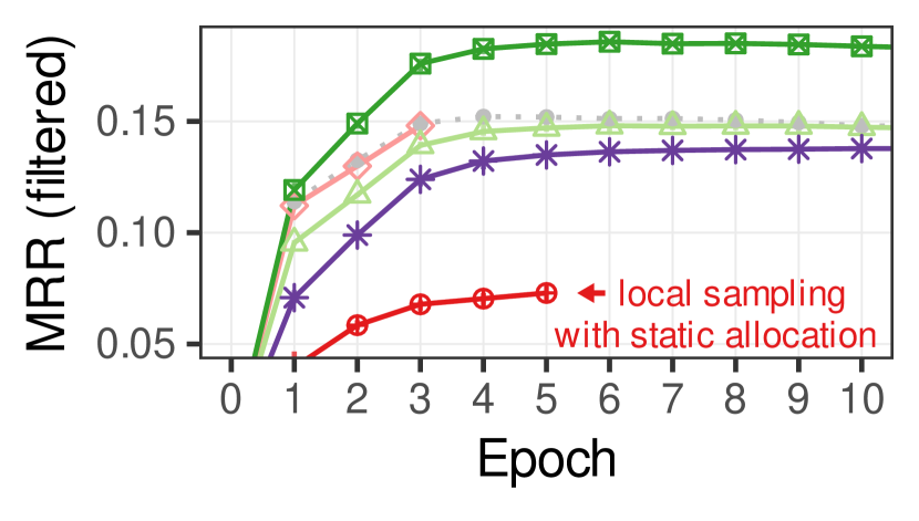
(c) KGE (quality over epoch)

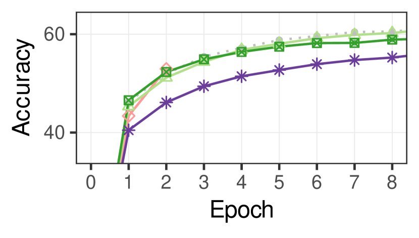
(d) WV (quality over epoch)

Figure 10. Performance of different sampling access management techniques. Both sample reuse and local sampling led to significant speedups over relocation.

5.5. Effect of Sampling Schemes

We investigated the effect of different sampling schemes in NuPS on run time and model quality. To do so, we ran KGE and WV with different sampling schemes: independent sampling (CONFORM), U=16 and U=64 sample reuse without postponing (BOUNDED) and with postponing (LONG-TERM), and local sampling (NON-CONFORM). Figures 10(a) and 10(b) show model quality over time, Figures 10(c) and 10(d) show model quality over epoch. We omit MF as it does not contain sampling access. We further omit the results from sample reuse with postponing as its results were within 10% of sample reuse without postponing. We found that both sample reuse and local sampling led to significant speedups over independent sampling, with small negative or—in the case of local sampling—even positive effects on per-epoch model quality.

Independent sampling provided per-epoch quality near-identical to the single node, but was slowest, because it induced high communication overhead for each sample. Sample reuse had lower communication overhead (and, thus, faster epoch run times), but at the cost of a (small) negative effect on per-epoch model quality. The higher the use frequency, the faster an epoch and the larger the negative effect on quality. The U=16 variant provided a good compromise, with minimal effect on model quality and fast run times.

Local sampling exhibited excellent performance, despite providing no guarantees on sampling quality: it was fast and per-epoch model quality was as good as the single node in WV, and was better in KGE. We hypothesize that this mainly is because NuPS combines local sampling with dynamic allocation: both tasks continuously relocate model parameters, such that the local parameter partitions contain many different parameters over time. To evaluate this hypothesis, we ran local sampling with static allocation in KGE. Figure 10(c) includes the results: with static allocation, model quality deteriorated drastically. We further conjecture that the reason for the better-than-single-node quality of local sampling in KGE was that relocation led to local samples that were more informative than global samples. Similar effects have been observed previously (Zheng et al., 2020).

5.6. Choice of Management Technique

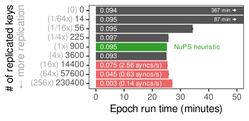
(a) KGE

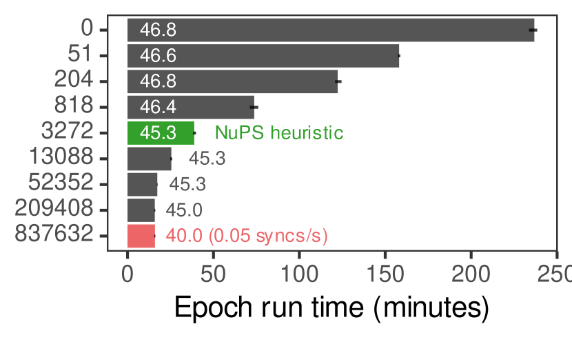
(b) WV

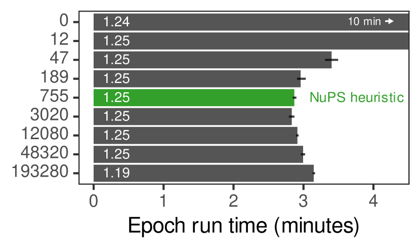
(c) MF

Figure 11. Impact of the management technique on epoch run time and model quality. The numbers in the plots depict model quality. A run is marked red if the resulting model quality was not within 10% of the model quality without replication. For these runs, the numbers in the plots additionally depict the actual synchronization frequency.

Table 3. Share of replicated keys, replica size, and share of accesses to replicas for different extents of replication. A cell is marked red if the resulting model quality was not within 10% of the quality without replication.

	Replicated keys (%)			Size of replicated values (MB)			Accesses to replicas (%)
Factor	KGE	WV	MF	KGE	WV	MF	KGE	WV	MF
0	$0.0000$	$0.0000$	$0.0000$	$0$	$0$	$0$	$0$	$0$	$0$
$1/64\text{\,}\mathrm{x}$	$0.0003$	$0.0027$	$0.0001$	$0$	$0$	$0$	$23$	$7$	$3$
$1/16\text{\,}\mathrm{x}$	$0.0012$	$0.0108$	$0.0004$	$0$	$1$	$0$	$33$	$13$	$5$
$1/4\text{\,}\mathrm{x}$	$0.0047$	$0.0435$	$0.0017$	$2$	$3$	$1$	$38$	$25$	$9$
$1\text{\,}\mathrm{x}$	$0.0187$	$0.1740$	$0.0069$	$7$	$12$	$6$	$41$	$45$	$14$
(heuristic)
$4\text{\,}\mathrm{x}$	$0.0747$	$0.6958$	$0.0275$	$27$	$50$	$23$	$44$	$67$	$19$
$16\text{\,}\mathrm{x}$	$0.2988$	$2.7832$	$0.1098$	$110$	$200$	$92$	$45$	$82$	$24$
$64\text{\,}\mathrm{x}$	$1.1951$	$11.1330$	$0.4393$	$439$	$799$	$369$	$47$	$88$	$30$
$256\text{\,}\mathrm{x}$	$4.7806$	$44.5319$	$1.7571$	$1758$	$3195$	$1475$	$52$	$92$	$37$

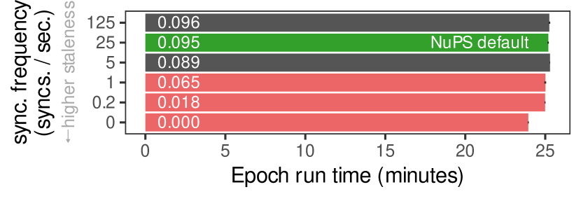
(a) KGE

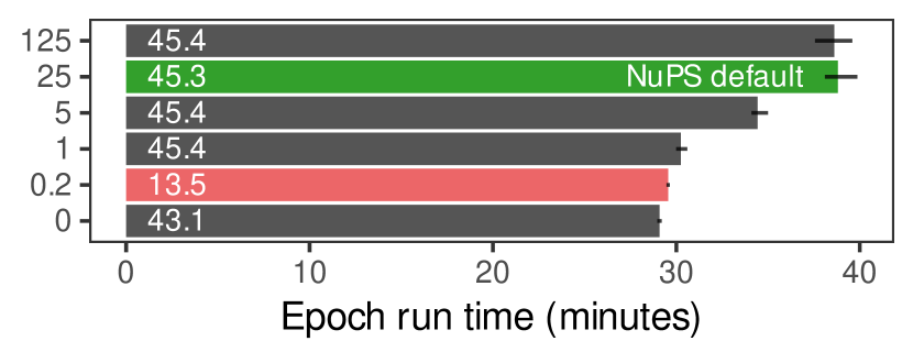
(b) WV

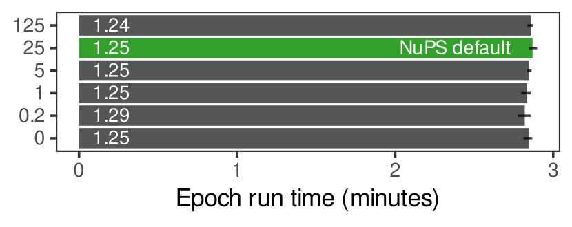
(c) MF

Figure 12. Effect of replica staleness on epoch run time and model quality. The numbers in the bars depict model quality after one epoch. Bars are marked red if model quality was not within 90% of the quality produced by a setting with no replication.

We investigated how the choice of management technique, i.e., the choice of whether to replicate or relocate a key, affects the performance of NuPS. The NuPS untuned heuristic replicates the $900$ most frequent keys in KGE, the $3272$ most frequent keys in WV, and the $755$ most frequent column keys in MF. We varied these numbers by factors $\frac{1}{64}$, $\frac{1}{16}$, $\frac{1}{4}$, $4$, $16$, $64$, and $256$. The leftmost columns of Table 3 depict what share of keys was replicated for each setting. We ran one epoch of each setting and measured epoch run time and model quality. Figure 11 depicts the results. We found that it was crucial for performance to replicate “enough” parameters such that the set of hot spot parameters is managed by replication, but not too many parameters, as replication created significant over-communication for long tail parameters.

This effect was visible for all tasks: starting from no replicated keys (i.e., all keys managed by relocation), increasing the number of replicated keys first improved run time, and had minimal effect on model quality. However, after some point, replicating more keys deteriorated model quality, and even slowed down run time for KGE and MF. The reason for the negative effect on model quality was that the replicas were stale, because the replica updates became too large to synchronize them frequently over the network of the cluster. We configured NuPS to provide the default $40\text{\,}\mathrm{m}\mathrm{s}$ staleness bound (i.e., 25 synchronizations per second), but to not block operations when it did not reach this goal. Figure 11 includes the actual synchronization frequency if model quality was not within 10% of the model quality without replication. The middle columns of Table 3 provide the size of the replicated values for all settings. For example, the 64x WV setting replicated $799\text{\,}\mathrm{M}\mathrm{B}$ of parameter values. Large numbers of replicated keys led to slower epoch run times for KGE and MF, because relocation operations competed with replica synchronization for network bandwidth. This effect was not visible for WV because, in WV, the majority of accesses went to replicated keys (and, thus, were fast despite network congestion). The share of accesses that went to replicas is depicted in the rightmost columns of Table 3. For example, 88% of all accesses went to replicas in the 64x WV setting.

5.7. Effect of Replica Staleness

We investigated the effect of replica staleness on epoch run time and model quality. To do so, we varied synchronization frequency: we synchronized replicas either 125, 25, 5, 1, or 0.2 times per second or not at all. We ran one epoch of each setting and measured epoch run time and model quality after this epoch. Note that without replica synchronization, nodes may hold different models. In these cases, we evaluated the model of the first node. Figure 12 reports the results. Overall, replication had only minimal effect on model quality when replica staleness was low.

Replication had only small effect on model quality when replicas were synchronized at least 5 times per second. In contrast, infrequent synchronization (less than once per second) deteriorated model quality drastically in KGE and WV. However, infrequent synchronization (or no synchronization at all) worked well in some settings (in particular in MF). We theorize that the reason for this was that NuPS employs replication for only a small subset of parameters, such that replication parameters are kept synchronized indirectly through the parameters that are managed by relocation.

5.8. Comparison to Task-Specific Implementations

In a general-purpose system, a performance overhead over optimized task-specific implementations is expected. To investigate the extent of this overhead in NuPS, we compared to specific implementations for each task. Each of these implementations is specialized and highly tuned for the respective task. In contrast to a general-purpose PS such as NuPS, these implementations cannot be used to run other ML tasks. Note that some of these implementations use different, more complex training algorithms than the implementations in NuPS. Overall, we found that NuPS was competitive to specialized and tuned task-specific implementations.

For MF, we compared to the highly tuned MPI implementations of DSGD and DSGD++ (Teflioudi et al., 2012). We ran convergence experiments on 8 and 16 nodes. We measured how long the implementations took to reach the 90% quality threshold. We used the same hyperparameters, model starting points, and learning rate schedule across DSGD, DSGD++, and NuPS. On 8 nodes, NuPS was 16% faster than DSGD and 15% slower than DSGD++. On 16 nodes, NuPS was 37% faster than DSGD and 16% faster than DSGD++.

For KGE, we compared to the highly specialized framework PyTorch-BigGraph (Lerer et al., 2019). Note that PyTorch-BigGraph is designed for a different training algorithm, with different hyperparameters: to reduce communication overhead, it uses mini-batch SGD, whereas the KGE implementation in NuPS employs regular SGD (i.e., batch size 1). To minimize the impact of algorithm hyperparameters in our comparison, we compared epoch run times. NuPS ran an epoch in 12 minutes on 16 nodes (24 minutes on 8 nodes). In this setting (i.e., batch size 1), PyTorch-BigGraph was much slower than NuPS: it took more than 5 hours to run one epoch, both on 8 and 16 nodes. Using a very large batch size led to faster epochs in PyTorch-BigGraph (up to 3x faster with batch size 1000 than NuPS with batch size 1), but can also be implemented in NuPS.

For WV, we are not aware of a highly tuned and publicly available distributed implementation, so we compared to two highly tuned single-node implementations: the original C implementation of Word2Vec (Mikolov et al., 2013) and Gensim (Řehůřek and Sojka, 2010). The implementation in Gensim and the one in NuPS are both based on the original C implementation. For both single-node implementations, we achieved the fastest epoch run times with 64 threads. Gensim completed an epoch in 15 minutes, the original implementation in 12 minutes. With 8x8 threads, NuPS took 13.5 minutes for one epoch; with 16x8 threads, it took 8 minutes. One factor that limits the performance of NuPS compared to these task-specific implementations is that—as other general-purpose PSs (Renz-Wieland et al., 2020)—NuPS provides per-key atomic updates. To achieve this, workers receive dedicated working copies of parameters. Creating these copies and writing updates back into the parameter store creates overhead compared to the task-specific WV implementations, which let workers read and write in the parameter store directly, without any consistency or isolation guarantees. Empirically, this works well for this particular task, but the effects for other tasks in a general-purpose system are unclear.

6. Conclusion

We explored how to extend the scope of PSs to ML with non-uniform parameter access. To this end, we presented NuPS, a non-uniform PS that employs multi-technique parameter management to efficiently handle skew and integrates sampling schemes to efficiently handle sampling. We found that a non-uniform PS can be highly beneficial: in our experimental study, NuPS outperformed existing PSs by up to one order of magnitude. These results open up several research directions for further improving PS performance: integrating more management techniques (e.g., highly specialized ones), developing further sampling schemes, and devising fine-grained methods for picking management techniques for parameters.

- (1)
- Abadi et al. (2016) Martín Abadi, Paul Barham, Jianmin Chen, Zhifeng Chen, Andy Davis, Jeffrey Dean, Matthieu Devin, Sanjay Ghemawat, Geoffrey Irving, Michael Isard, Manjunath Kudlur, Josh Levenberg, Rajat Monga, Sherry Moore, Derek Murray, Benoit Steiner, Paul Tucker, Vijay Vasudevan, Pete Warden, Martin Wicke, Yuan Yu, and Xiaoqiang Zheng. 2016. TensorFlow: A System for Large-scale Machine Learning. In Proceedings of the 12th Conference on Operating Systems Design and Implementation (OSDI ’16). 265–283.
- Ahmed et al. (2012) Amr Ahmed, Moahmed Aly, Joseph Gonzalez, Shravan Narayanamurthy, and Alexander Smola. 2012. Scalable Inference in Latent Variable Models. In Proceedings of the 5th ACM International Conference on Web Search and Data Mining (WSDM ’12). 123–132.
- Bamler and Mandt (2020) Robert Bamler and Stephan Mandt. 2020. Extreme Classification via Adversarial Softmax Approximation. In Proceedings of the 8th International Conference on Learning Representations (ICLR ’20).
- Battiti (1989) Roberto Battiti. 1989. Accelerated Backpropagation Learning: Two Optimization Methods. Complex systems 3, 4 (1989), 331–342.
- Broscheit et al. (2020) Samuel Broscheit, Daniel Ruffinelli, Adrian Kochsiek, Patrick Betz, and Rainer Gemulla. 2020. LibKGE - A Knowledge Graph Embedding Library for Reproducible research. In Proceedings of the 2020 Conference on Empirical Methods in Natural Language Processing: System Demonstrations. 165–174.
- Chechik et al. (2010) Gal Chechik, Varun Sharma, Uri Shalit, and Samy Bengio. 2010. Large Scale Online Learning of Image Similarity Through Ranking. Journal of Machine Learning Research 11, 36 (2010), 1109–1135.
- Chelba et al. (2013) Ciprian Chelba, Tomas Mikolov, Mike Schuster, Qi Ge, Thorsten Brants, and Phillipp Koehn. 2013. One Billion Word Benchmark for Measuring Progress in Statistical Language Modeling. CoRR abs/1312.3005 (2013). arXiv:1312.3005
- Chen et al. (2015) Tianqi Chen, Mu Li, Yutian Li, Min Lin, Naiyan Wang, Minjie Wang, Tianjun Xiao, Bing Xu, Chiyuan Zhang, and Zheng Zhang. 2015. MXNet: A Flexible and Efficient Machine Learning Library for Heterogeneous Distributed Systems. CoRR abs/1512.01274 (2015). arXiv:1512.01274
- Cheng et al. (2016) Wenliang Cheng, Chengyu Wang, Bing Xiao, Weining Qian, and Aoying Zhou. 2016. On Statistical Characteristics of Real-Life Knowledge Graphs. In Big Data Benchmarks, Performance Optimization, and Emerging Hardware, Jianfeng Zhan, Rui Han, and Roberto V. Zicari (Eds.). 37–49.
- Chilimbi et al. (2014) Trishul Chilimbi, Yutaka Suzue, Johnson Apacible, and Karthik Kalyanaraman. 2014. Project Adam: Building an Efficient and Scalable Deep Learning Training System. In Proceedings of the 11th Conference on Operating Systems Design and Implementation (OSDI ’14). 571–582.
- Ciciani et al. (1990) Bruno Ciciani, Daniel Dias, and Philip Yu. 1990. Analysis of Replication in Distributed Database Systems. IEEE Transactions on Knowledge & Data Engineering 2, 02 (April 1990), 247–261.
- Clauset et al. (2009) Aaron Clauset, Cosma Rohilla Shalizi, and M. E. J. Newman. 2009. Power-Law Distributions in Empirical Data. SIAM Rev. 51, 4 (2009), 661–703.
- Cui et al. (2014) Henggang Cui, Alexey Tumanov, Jinliang Wei, Lianghong Xu, Wei Dai, Jesse Haber-Kucharsky, Qirong Ho, Gregory Ganger, Phillip Gibbons, Garth Gibson, and Eric Xing. 2014. Exploiting Iterative-ness for Parallel ML Computations. In Proceedings of the ACM Symposium on Cloud Computing (SOCC ’14). Article 5.
- Dai et al. (2015) Wei Dai, Abhimanu Kumar, Jinliang Wei, Qirong Ho, Garth Gibson, and Eric P Xing. 2015. High-Performance Distributed ML at Scale through Parameter Server Consistency Models. In Proceedings of the 29th AAAI Conference on Artificial Intelligence (AAAI ’15). 79–87.
- Dean et al. (2012) Jeffrey Dean, Greg Corrado, Rajat Monga, Kai Chen, Matthieu Devin, Quoc Le, Mark Mao, Marc’Aurelio Ranzato, Andrew Senior, Paul Tucker, Ke Yang, and Andrew Ng. 2012. Large Scale Distributed Deep Networks. In Proceedings of the 25th International Conference on Neural Information Processing Systems (NIPS ’12). 1223–1231.
- Devlin et al. (2019) Jacob Devlin, Ming-Wei Chang, Kenton Lee, and Kristina Toutanova. 2019. BERT: Pre-training of Deep Bidirectional Transformers for Language Understanding. In Proceedings of the 2019 Conference of the North American Chapter of the Association for Computational Linguistics: Human Language Technologies. 4171–4186.
- Dowdy and Foster (1982) Lawrence W. Dowdy and Derrell V. Foster. 1982. Comparative Models of the File Assignment Problem. ACM Comput. Surv. 14, 2 (June 1982), 287–313.
- Duchi et al. (2011) John Duchi, Elad Hazan, and Yoram Singer. 2011. Adaptive Subgradient Methods for Online Learning and Stochastic Optimization. Journal of Machine Learning Research 12 (July 2011), 2121–2159.
- El Abbadi (1991) A. El Abbadi. 1991. Adaptive protocols for managing replicated distributed databases. In Proceedings of the 3rd IEEE Symposium on Parallel and Distributed Processing. 36–43.
- Faloutsos et al. (1999) Michalis Faloutsos, Petros Faloutsos, and Christos Faloutsos. 1999. On Power-Law Relationships of the Internet Topology. In Proceedings of the Conference on Applications, Technologies, Architectures, and Protocols for Computer Communication (SIGCOMM ’99). 251–262.
- Gonzalez et al. (2012) Joseph Gonzalez, Yucheng Low, Haijie Gu, Danny Bickson, and Carlos Guestrin. 2012. PowerGraph: Distributed Graph-parallel Computation on Natural Graphs. In Proceedings of the 10th Conference on Operating Systems Design and Implementation (OSDI ’12). 17–30.
- Grover and Leskovec (2016) Aditya Grover and Jure Leskovec. 2016. Node2vec: Scalable Feature Learning for Networks. In Proceedings of the 22nd ACM SIGKDD International Conference on Knowledge Discovery and Data Mining (KDD ’16). 855–864.
- Hashemi et al. (2019) Sayed Hadi Hashemi, Sangeetha Abdu Jyothi, and Roy Campbell. 2019. TicTac: Accelerating Distributed Deep Learning with Communication Scheduling. In Proceedings of Machine Learning and Systems (MLSys ’19, Vol. 1), A. Talwalkar, V. Smith, and M. Zaharia (Eds.). 418–430.
- Ho et al. (2013) Qirong Ho, James Cipar, Henggang Cui, Jin Kyu Kim, Seunghak Lee, Phillip Gibbons, Garth Gibson, Gregory Ganger, and Eric Xing. 2013. More Effective Distributed ML via a Stale Synchronous Parallel Parameter Server. In Proceedings of the 26th International Conference on Neural Information Processing Systems (NIPS ’13). 1223–1231.
- Howard and Ruder (2018) Jeremy Howard and Sebastian Ruder. 2018. Universal Language Model Fine-tuning for Text Classification. In Proceedings of the 56th Annual Meeting of the Association for Computational Linguistics (ACL ’18). 328–339.
- Huang et al. (2018) Yuzhen Huang, Tatiana Jin, Yidi Wu, Zhenkun Cai, Xiao Yan, Fan Yang, Jinfeng Li, Yuying Guo, and James Cheng. 2018. FlexPS: Flexible Parallelism Control in Parameter Server Architecture. PVLDB 11, 5 (Jan. 2018), 566–579.
- Jagerman et al. (2017) Rolf Jagerman, Carsten Eickhoff, and Maarten de Rijke. 2017. Computing Web-scale Topic Models Using an Asynchronous Parameter Server. In Proceedings of the 40th International ACM SIGIR Conference on Research and Development in Information Retrieval (SIGIR ’17). 1337–1340.
- Jayarajan et al. (2019) Anand Jayarajan, Jinliang Wei, Garth Gibson, Alexandra Fedorova, and Gennady Pekhimenko. 2019. Priority-based Parameter Propagation for Distributed DNN Training. In Proceedings of Machine Learning and Systems (MLSys ’19, Vol. 1), A. Talwalkar, V. Smith, and M. Zaharia (Eds.). 132–145.
- Ji et al. (2019) S. Ji, N. Satish, S. Li, and P. K. Dubey. 2019. Parallelizing Word2Vec in Shared and Distributed Memory. IEEE Transactions on Parallel and Distributed Systems 30, 9 (2019), 2090–2100.
- Jiang et al. (2017) Jiawei Jiang, Bin Cui, Ce Zhang, and Lele Yu. 2017. Heterogeneity-Aware Distributed Parameter Servers. In Proceedings of the 2017 ACM International Conference on Management of Data (SIGMOD ’17). 463–478.
- Jiang et al. (2020) Yimin Jiang, Yibo Zhu, Chang Lan, Bairen Yi, Yong Cui, and Chuanxiong Guo. 2020. A Unified Architecture for Accelerating Distributed DNN Training in Heterogeneous GPU/CPU Clusters. In 14th USENIX Symposium on Operating Systems Design and Implementation (OSDI ’20). 463–479.
- Kim et al. (2019) Jin Kyu Kim, Abutalib Aghayev, Garth Gibson, and Eric Xing. 2019. STRADS-AP: Simplifying Distributed Machine Learning Programming without Introducing a New Programming Model. In Proceedings of the 2019 USENIX Annual Technical Conference (USENIX ’19). 207–222.
- Kim et al. (2016) Jin Kyu Kim, Qirong Ho, Seunghak Lee, Xun Zheng, Wei Dai, Garth Gibson, and Eric Xing. 2016. STRADS: A Distributed Framework for Scheduled Model Parallel Machine Learning. In Proceedings of the 11th European Conference on Computer Systems (EuroSys ’16). Article 5.
- Kochsiek and Gemulla (2021) Adrian Kochsiek and Rainer Gemulla. 2021. Parallel Training of Knowledge Graph Embedding Models: A Comparison of Techniques. PVLDB 15, 3 (Nov 2021), 633–645.
- Koren et al. (2009) Yehuda Koren, Robert Bell, and Chris Volinsky. 2009. Matrix Factorization Techniques for Recommender Systems. Computer 42, 8 (Aug. 2009), 30–37.
- LeCun et al. (1989) Y. LeCun, B. Boser, J. S. Denker, D. Henderson, R. E. Howard, W. Hubbard, and L. D. Jackel. 1989. Backpropagation Applied to Handwritten Zip Code Recognition. Neural Comput. 1, 4 (Dec. 1989), 541–551.
- Lerer et al. (2019) Adam Lerer, Ledell Wu, Jiajun Shen, Timothee Lacroix, Luca Wehrstedt, Abhijit Bose, and Alex Peysakhovich. 2019. PyTorch-BigGraph: A Large-scale Graph Embedding System. In Proceedings of the 2nd SysML Conference (SysML ’19).
- Li et al. (2014) Mu Li, David Andersen, Jun Woo Park, Alexander Smola, Amr Ahmed, Vanja Josifovski, James Long, Eugene Shekita, and Bor-Yiing Su. 2014. Scaling Distributed Machine Learning with the Parameter Server. In Proceedings of the 11th Conference on Operating Systems Design and Implementation (OSDI ’14). 583–598.
- Lian et al. (2015) Xiangru Lian, Yijun Huang, Yuncheng Li, and Ji Liu. 2015. Asynchronous Parallel Stochastic Gradient for Nonconvex Optimization. In Proceedings of the 28th International Conference on Neural Information Processing Systems (NIPS’15). 2737–2745.
- Liu et al. (2017) Hanxiao Liu, Yuexin Wu, and Yiming Yang. 2017. Analogical Inference for Multi-relational Embeddings. In Proceedings of the 34th International Conference on Machine Learning (ICML ’17). 2168–2178.
- Liu et al. (2018) Xiaodong Liu, Yelong Shen, Kevin Duh, and Jianfeng Gao. 2018. Stochastic Answer Networks for Machine Reading Comprehension. In Proceedings of the 56th Annual Meeting of the Association for Computational Linguistics (ACL ’18). 1694–1704.
- Low et al. (2012) Yucheng Low, Danny Bickson, Joseph Gonzalez, Carlos Guestrin, Aapo Kyrola, and Joseph Hellerstein. 2012. Distributed GraphLab: A Framework for Machine Learning and Data Mining in the Cloud. PVLDB 5, 8 (April 2012), 716–727.
- Makari et al. (2015) Faraz Makari, Christina Teflioudi, Rainer Gemulla, Peter Haas, and Yannis Sismanis. 2015. Shared-memory and shared-nothing stochastic gradient descent algorithms for matrix completion. Knowledge and Information Systems 42, 3 (01 Mar 2015), 493–523.
- Meka et al. (2009) Raghu Meka, Prateek Jain, and Inderjit Dhillon. 2009. Matrix Completion from Power-Law Distributed Samples. In Advances in Neural Information Processing Systems, Y. Bengio, D. Schuurmans, J. Lafferty, C. Williams, and A. Culotta (Eds.), Vol. 22. 1258–1266.
- Mikolov et al. (2013) Tomas Mikolov, Kai Chen, Greg Corrado, and Jeffrey Dean. 2013. Efficient Estimation of Word Representations in Vector Space. In Proceedings of the 1st International Conference on Learning Representations (ICLR ’13).
- Mohamed et al. (2020) Aisha Mohamed, Shameem Parambath, Zoi Kaoudi, and Ashraf Aboulnaga. 2020. Popularity Agnostic Evaluation of Knowledge Graph Embeddings. In Proceedings of the 36th Conference on Uncertainty in Artificial Intelligence (UAI ’20). 1059–1068.
- Moreno-Sánchez et al. (2016) Isabel Moreno-Sánchez, Francesc Font-Clos, and Álvaro Corral. 2016. Large-Scale Analysis of Zipf’s Law in English Texts. PloS one 11, 1 (22 Jan 2016).
- Nickel et al. (2016) Maximilian Nickel, Kevin Murphy, Volker Tresp, and Evgeniy Gabrilovich. 2016. A Review of Relational Machine Learning for Knowledge Graphs. Proc. IEEE 104, 1 (Jan 2016), 11–33.
- Nickel et al. (2011) Maximilian Nickel, Volker Tresp, and Hans-Peter Kriegel. 2011. A Three-way Model for Collective Learning on Multi-relational Data. In Proceedings of the 28th International Conference on Machine Learning (ICML ’11). 809–816.
- Pascanu et al. (2013) Razvan Pascanu, Tomas Mikolov, and Yoshua Bengio. 2013. On the Difficulty of Training Recurrent Neural Networks. In Proceedings of the 30th International Conference on Machine Learning (ICML ’13). 1310–1318.
- Pennington et al. (2014) Jeffrey Pennington, Richard Socher, and Christopher Manning. 2014. GloVe: Global Vectors for Word Representation. In Proceedings of the 2014 Conference on Empirical Methods in Natural Language Processing (EMNLP) (ACL ’14). 1532–1543.
- Peters et al. (2018) Matthew Peters, Mark Neumann, Mohit Iyyer, Matt Gardner, Christopher Clark, Kenton Lee, and Luke Zettlemoyer. 2018. Deep Contextualized Word Representations. In Proceedings of the 2018 Conference of the North American Chapter of the Association for Computational Linguistics: Human Language Technologies (NAACL ’18). 2227–2237.
- Rawat et al. (2021) Ankit Singh Rawat, Aditya Krishna Menon, Wittawat Jitkrittum, Sadeep Jayasumana, Felix X. Yu, Sashank J. Reddi, and Sanjiv Kumar. 2021. Disentangling Sampling and Labeling Bias for Learning in Large-Output Spaces. CoRR abs/2105.05736 (2021). arXiv:2105.05736
- Řehůřek and Sojka (2010) Radim Řehůřek and Petr Sojka. 2010. Software Framework for Topic Modelling with Large Corpora. In Proceedings of the LREC 2010 Workshop on New Challenges for NLP Frameworks (LREC ’10). 45–50.
- Rendle et al. (2009) Steffen Rendle, Christoph Freudenthaler, Zeno Gantner, and Lars Schmidt-Thieme. 2009. BPR: Bayesian Personalized Ranking from Implicit Feedback. In Proceedings of the 25th Conference on Uncertainty in Artificial Intelligence (UAI ’09). 452–461.
- Renz-Wieland et al. (2021) Alexander Renz-Wieland, Tobias Drobisch, Zoi Kaoudi, Rainer Gemulla, and Volker Markl. 2021. Just Move It! Dynamic Parameter Allocation in Action. PVLDB 14, 12 (Jul 2021), 2707–2710.
- Renz-Wieland et al. (2020) Alexander Renz-Wieland, Rainer Gemulla, Steffen Zeuch, and Volker Markl. 2020. Dynamic Parameter Allocation in Parameter Servers. PVLDB 13, 12 (July 2020), 1877–1890.
- Ruffinelli et al. (2020) Daniel Ruffinelli, Samuel Broscheit, and Rainer Gemulla. 2020. You CAN Teach an Old Dog New Tricks! On Training Knowledge Graph Embeddings. In Proceedings of the 8th International Conference on Learning Representations (ICLR ’20).
- Schroff et al. (2015) F. Schroff, D. Kalenichenko, and J. Philbin. 2015. FaceNet: A unified embedding for face recognition and clustering. In 2015 IEEE Conference on Computer Vision and Pattern Recognition (CVPR ’15). 815–823.
- Smola and Narayanamurthy (2010) Alexander Smola and Shravan Narayanamurthy. 2010. An Architecture for Parallel Topic Models. PVLDB 3, 1-2 (Sept. 2010), 703–710.
- Socher et al. (2013) Richard Socher, John Bauer, Christopher Manning, and Andrew Ng. 2013. Parsing with Compositional Vector Grammars. In Proceedings of the 51st Annual Meeting of the Association for Computational Linguistics (ACL ’13). 455–465.
- Stergiou et al. (2017) Stergios Stergiou, Zygimantas Straznickas, Rolina Wu, and Kostas Tsioutsiouliklis. 2017. Distributed Negative Sampling for Word Embeddings. In Proceedings of the 31st AAAI Conference on Artificial Intelligence (AAAI ’17). 2569–2575.
- Teflioudi et al. (2012) Christina Teflioudi, Faraz Makari, and Rainer Gemulla. 2012. Distributed Matrix Completion. In 2012 IEEE 12th International Conference on Data Mining (ICDM ’12). 655–664.
- Träff (2010) Jesper Larsson Träff. 2010. Transparent Neutral Element Elimination in MPI Reduction Operations. In Recent Advances in the Message Passing Interface, Rainer Keller, Edgar Gabriel, Michael Resch, and Jack Dongarra (Eds.). 275–284.
- Trouillon et al. (2016) Théo Trouillon, Johannes Welbl, Sebastian Riedel, Éric Gaussier, and Guillaume Bouchard. 2016. Complex Embeddings for Simple Link Prediction. In Proceedings of the 33rd International Conference on Machine Learning (ICML ’16). 2071–2080.
- Wang et al. (2019) Xiaozhi Wang, Tianyu Gao, Zhaocheng Zhu, Zhiyuan Liu, Juanzi Li, and Jian Tang. 2019. KEPLER: A Unified Model for Knowledge Embedding and Pre-trained Language Representation. CoRR abs/1911.06136 (2019). arXiv:1911.06136
- Wolfson and Jajodia (1992) Ouri Wolfson and Sushil Jajodia. 1992. Distributed Algorithms for Dynamic Replication of Data. In Proceedings of the 11fh ACM SIGACT-SIGMOD-SIGART Symposium on Principles of Database Systems (PODS ’92). 149–163.
- Xing et al. (2015) Eric Xing, Qirong Ho, Wei Dai, Jin-Kyu Kim, Jinliang Wei, Seunghak Lee, Xun Zheng, Pengtao Xie, Abhimanu Kumar, and Yaoliang Yu. 2015. Petuum: A New Platform for Distributed Machine Learning on Big Data. In Proceedings of the 21th ACM SIGKDD International Conference on Knowledge Discovery and Data Mining (KDD ’15). 1335–1344.
- Yang et al. (2020) Zhen Yang, Ming Ding, Chang Zhou, Hongxia Yang, Jingren Zhou, and Jie Tang. 2020. Understanding Negative Sampling in Graph Representation Learning. In Proceedings of the 26th ACM SIGKDD International Conference on Knowledge Discovery and Data Mining (KDD ’20). 1666–1676.
- Zhang et al. (2017) Hao Zhang, Zeyu Zheng, Shizhen Xu, Wei Dai, Qirong Ho, Xiaodan Liang, Zhiting Hu, Jinliang Wei, Pengtao Xie, and Eric P. Xing. 2017. Poseidon: An Efficient Communication Architecture for Distributed Deep Learning on GPU Clusters. In 2017 USENIX Annual Technical Conference (ATC ’17). 181–193.
- Zhang et al. (2018) Xin Zhang, Jia Liu, and Zhengyuan Zhu. 2018. Taming Convergence for Asynchronous Stochastic Gradient Descent with Unbounded Delay in Non-Convex Learning. CoRR abs/1805.09470 (2018). arXiv:1805.09470
- Zhang et al. (2019) Zhipeng Zhang, Bin Cui, Yingxia Shao, Lele Yu, Jiawei Jiang, and Xupeng Miao. 2019. PS2: Parameter Server on Spark. In Proceedings of the 2019 ACM International Conference on Management of Data (SIGMOD ’19). 376–388.
- Zheng et al. (2020) Da Zheng, Xiang Song, Chao Ma, Zeyuan Tan, Zihao Ye, Jin Dong, Hao Xiong, Zheng Zhang, and George Karypis. 2020. DGL-KE: Training Knowledge Graph Embeddings at Scale. CoRR abs/2004.08532 (2020). arXiv:2004.08532