Spin dynamic response to a time dependent field

Abstract

The dynamic response of a parametric system constituted by a spin precessing in a time dependent magnetic field is studied by means of a perturbative approach that unveils unexpected features, and is then experimentally validated. The first-order analysis puts in evidence different regimes: beside a tailorable low-pass-filter behaviour, a band-pass response with interesting potential applications emerges. Extending the analysis to the second perturbation order permits to study the response to generically oriented fields and to characterize several non-linear features in the behaviour of such kind of systems.

I Introduction

Optical atomic magnetometers (OAMs) can be used to detect time dependent fields (TDF) that can be fast varying, disadvantageoulsy oriented and not necessarily small. Several kinds of optical magnetometers reach their best performance when measuring weak and quasi-static fields. These systems are often modelled and analyzed under these conditions, and their behaviour in the above mentioned, more general case is scarcely discussed and investigated.

The possibility of measuring magnetic fields using optical pumping and probing of alkali atoms was pointed out more than 60 years ago, in the works of Dehmelt demhelt_pr_57 and Bell and Bloom bellandbloom_pr_57 ; bell_prl_61 . In the late Sixties and Seventies, important further steps were carried out by the group of Cohen-Tannoudji dupont_rpa_70 ; dupont_pla_69 . The mentioned works demonstrated the potential for high resolution magnetometry based on magneto-optical effects which were known since the historical observations described by Michael Faraday faraday_1848 in non-resonant high density materials, and by Macaluso and Corbino macaluso_98 ; macaluso_99 , who observed the enhancement of the Faraday effect under resonant conditions in low density material (atomic media).

Advances in laser technology and in laser spectroscopy, in conjunction with intense studies on optical pumping processes happer_rmp_72 ; happer_book_10 prepared a revival of optical magnetometry at the beginning of this millennium alexandrov_lp_96 . The practicality and the potential of this research in applications, was induced by further technological advances, making available easy-to-use (reliable, low-cost, low-power, small size, highly tunable and stable) solid state laser sources, and high-quality atomic samples with long ground-state relaxation times. Many research groups contributed to this new phase of optical magnetometry, and a panoramic view of that recent history can be found in budker_natph_07 .

Optical magnetometers are developed for a variety of applications Savukov_intech_10 including fundamental research Swank_pra_18 ; guarrera_prl_20 ; abel_pra_20 , characterization of magnetic anomalies and of their dynamics in space-physics korth_jgr_16 ; pollinger_mst_18 , geology prouty_book_2013 , archaeology fassbinder_encyarch_17 ; mathe_as_17 , material science e.g. to detect diluted magnetic nano- and micro-particles jaufenthaler_sens_20 or induced eddy currents marmugi_apl_19 ; jensen_prr_19 ; bevington_jap_19 (with potential in medical applications, in detection of biomagnetism baranga_apl_06 or in building apparatuses for nuclear magnetic resonance (for spectroscopy or imaging) in the ultra-low-field savukov_prl_05 ; biancalana_DH_jpcl_17 ; tayler_jmr_19 ; biancalana_apl_19 and zero-to-ultra-low field regimes blanchard_jmr_20 ; xu_pnas_06 .

Among the most attractive characteristics of OAMs is their robustness and the possibility of pushing to extreme levels many crucial parameters such as sensitivity, size, minimal power consumption, bandwidth, long-term operativity, etc. The high sensitivity of atomic magnetometers relies on the fact that light near-resonant with an optical transition may create long-lived magnetization in the atomic ground state that subsequently evolves under the effect of the magnetic field that is being measured. This precession in turn modifies the optical properties of the atomic medium, and can be detected by absorption and/or polarimetric measurements performed on a probe radiation propagated through the medium itself.

Regardless of the quantum or the classical approach to the problem, the evolution of a spin precessing in a magnetic field is well described by the Larmor equations, or by the Bloch equations when spin relaxation processes play important role. This magnetic-resonance picture is actually the framework in which the spin dynamics in OAM can be described.

When dealing with time-dependent fields, the problem is often considered in the resonant regime, when a field component oscillates at the Larmor frequency (this is the case of radio-frequency magnetometers). Other studies, concerning fast oscillating fields, consider the magnetic dressing phenomena, which address configurations with a strong field that oscillates at frequencies largely above the Larmor one. At the other extreme, the quasi-stationary regime is analyzed (e.g. in the case of light-modulated OAMs), which let detect slow and extremely weak field variations.

When considering a quasi-static TDF $\mathbf{b}$ much weaker than the static field $\mathbf{B}_{L}$ to which it is superimposed, the scalar nature of OAM makes them responsive only to the longitudinal TDF component: the Larmor frequency $\omega_{L}$ depends of the field modulus via the gyromagnetic factor $\gamma$ according to

$$\omega_{L}=\gamma|\mathbf{B}|=\gamma\sqrt{(\mathbf{B}_{L}+\mathbf{b})\cdot(\mathbf{B}_{L}+\mathbf{b})}\approx\gamma(B_{L}+\delta b_{\parallel}),$$ (1)

to a first-order Taylor expansion in the quantity $b_{\parallel}/B_{L}$, being $b_{\parallel}$ the component of $\mathbf{b}$ along the direction of $\mathbf{B}_{L}$. The high sensitivity of OAM makes indeed these detectors excellent tools to detect very slow and extremly weak TDFs. The weak- and low-frequency field approximation leading to Eq. 1 is often implicitly assumed wilson_prr_20 ; jensen_sr_18 : the dynamic response to stronger, generically oriented and/or non quasi-static TDF remains overlooked. Only few works address operating conditions with TDF not necessarily small, with fast dynamics and generic orientation ingleby_pra_17 ; wilson_prr_20 , and this investigation –with emphasis to the system response– is at the focus of the present work.

If we consider a Bell and Bloom magnetometer driven at resonance, a slight change of the magnetic field modulus will bring the device to a near-resonant regime, with a correspondent new (near-resonant) steady state characterized by smaller and dephased atomic magnetization. However, we are not dealing with a linear time-invariant (LTI) system forced by a signal initially resonant and then out-of-resonance. The magnetometer should be rather regarded (see also the appendix in ref. Savukov_mst_17 ) as a parametric system forced by a stationary term. Despite the inherent similarity at the steady state, the transient response of such a system cannot be studied in terms of a damped-forced (LTI) device.

Parametric systems are used in a variety of sensors e.g. for nanoscale mass and acceleration detectors villanueva_nl_11 , solid state gyroscopes feng_ieee_04 , micropositioning santhosh_pt_12 . In some cases instabilities of parametric oscillators can be used to sustain the sensor surappa_apl_17 , which is viable technique when the equation ruling the dynamics makes it possible to provide the system with energy from the parameter modulation. This is the case of many parametric oscillators, but it is not a general feature and does not apply to the particular case of precessing spins. The dynamic response of a parametric system to the parameter(s) variation depends strictly on its nature and requires a dedicated analysis of the equations that rule its dynamics.

This work provides an accurate description of the dynamical behaviour of spins precessing in a TDF. Similarly to the case of Ref.ding_sens_18 , a Bell and Bloom magnetometer is considered as a test of the developed model, under conditions in which the driving field $\mathbf{B}$ changes in time with TDF components both parallel and transverse with respect to the static (bias) term. The field is assumed to vary not necessarily slowly and by small but not necessarily vanishing amounts. Differing from Ref.ding_sens_18 , which reports a numerical study, in the Sec. II we develop an analytic perturbative model to evaluate the response of such system to TDFs.

In Sec. III we describe an experimental setup, where a weak synchronous optical pumping acting on an atomic vapour compensates the relaxation phenomena, rendering the evolution of the sample magnetization adequately described by the Larmor precession equation. The Sec. IV reports a quantitative analysis and experimental tests of the main outputs of the model. A synthesis of the main findings is finally drawn in the Sec. V.

II Model

symbol	description
$\gamma$	gyromagnetic factor
$\omega_{L}=\gamma|B_{L}|$	Larmor angular frequency in the static field
$\omega$	angular frequency of the modulating signal
$\Gamma$	relaxation rate
$\mathbf{M}$	magnetization
$i=1,2,3$	indexes corresponding to $x,y,z$ directions
$b_{i}=\omega_{i}/\gamma$	time dependent field components
$f(t)=\sum_{n}f_{n}\operatorname{\displaystyle e}^{in\omega t}$	forcing term
$w_{i}$	amplitudes of oscillating $b_{i}$
$a_{k},\varphi_{k}$	amplitude and phase of the polarimetric signal, at the $k$th order
$\Omega_{i,k}$	Fourier angular frequencies of the $i$th component of b

Table 1: Symbols

The starting point in modeling of the spin response is the Larmor equation for the magnetization vector

$$\dot{\mathbf{M}}=-\Gamma\mathbf{M}+\gamma\mathbf{B}(t)\times\mathbf{M}+\mathbf{f}(t)$$ (2)

where $\gamma$ is the gyromagnetic factor and $\mathbf{f}(t)$ represents the action of the circularly polarized pump radiation and it is modeled as a forcing term (a list of symbol definitions is reported in Tab.1). The total magnetic field $\mathbf{B}$ is composed of a large static one $\mathbf{B}_{L}$ (bias field) perpendicular to the pump radiation wavevector and a small TDF $\mathbf{b}(t)$. A simplified isotropic decay mechanism ($-\Gamma\mathbf{M}$) is included. This is a well justified approximation as discussed in biancalana_apb_16 . Fixing the axis in such a way that the $x$ axis is along the pump and the $y$ axis is along the bias field $\mathbf{B}_{L}$ one obtains the equations

$$\dot{M}_{+} =-\Gamma M_{+}-i(\omega_{L}+\omega_{2}(t))M_{+}+(i\omega_{1}(t)-\omega_{3}(t))M_{2}+f(t)$$ (3a)

$$\dot{M}_{-} =-\Gamma M_{-}+i(\omega_{L}+\omega_{2}(t))M_{-}-(i\omega_{1}(t)+\omega_{3}(t))M_{2}+f(t)$$ (3b)

$$\dot{M}_{2} =-\Gamma M_{2}+\frac{1}{2}(i\omega_{1}(t)+\omega_{3}(t))M_{+}-\frac{1}{2}(i\omega_{1}(t)-\omega_{3}(t))M_{-}$$ (3c)

where $M_{\pm}=M_{x}\pm iM_{z}$, $M_{2}=M_{y}$, $\omega_{L}=\gamma B_{L}$ and $\omega_{i}(t)=\gamma b_{i}(t)$. These equations must be solved in the regime of $\omega_{i}(t)\ll\omega_{L}$, which can be rewritten in matrix form as

$$\begin{split}\dot{\mathbf{M}}&=-\Gamma\mathbf{M}+\begin{pmatrix}-i\omega_{L}&0&0\\ 0&i\omega_{L}&0\\ 0&0&0\end{pmatrix}\mathbf{M}+\epsilon\begin{pmatrix}-i\omega_{2}&0&i\omega_{+}\\ 0&i\omega_{2}&-i\omega_{-}\\ i\omega_{-}/2&-i\omega_{+}/2&0\end{pmatrix}\mathbf{M}+f(t)\begin{pmatrix}1\\ 1\\ 0\end{pmatrix}\\ &=-\Gamma\mathbf{M}+(A_{0}+\epsilon A_{1}(t))\mathbf{M}+f(t)\mathbf{u}\end{split}$$ (4)

here we have slightly redefined the magnetization as $\mathbf{M}=(M_{+},M_{-},M_{2})$ and introduced $\omega_{\pm}(t)=\omega_{1}(t)\pm i\omega_{3}(t)$. The parameter $\epsilon$ is just a bookkeeping device for the perturbation theory. In fact writing $\mbox{$\mathbf{M}$}=\mbox{$\mathbf{M}^{(0)}$}+\epsilon\mbox{$\mathbf{M}^{(1)}$}+\epsilon^{2}\mbox{$\mathbf{M}^{(2)}$}+\ldots$ we have

$$\dot{\mathbf{M}}^{(0)} =-\Gamma\mbox{$\mathbf{M}^{(0)}$}+A_{0}\mbox{$\mathbf{M}^{(0)}$}+\mathbf{u}f(t)$$ (5a)

$$\dot{\mathbf{M}}^{(1)} =-\Gamma\mbox{$\mathbf{M}^{(1)}$}+A_{0}\mbox{$\mathbf{M}^{(1)}$}+A_{1}(t)\mbox{$\mathbf{M}^{(0)}$}$$ (5b)

$$\dot{\mathbf{M}}^{(2)} =-\Gamma\mbox{$\mathbf{M}^{(2)}$}+A_{0}\mbox{$\mathbf{M}^{(2)}$}+A_{1}(t)\mbox{$\mathbf{M}^{(1)}$}$$ (5c)

The steady-state solution for $\mathbf{M}^{(0)}$can be obtained noticing that the function $f(t)$ is a real and periodic function (whose exact form is not important as it is shown below) which represents the modulated pumping

$$f(t)=\sum_{n}f_{n}\operatorname{\displaystyle e}^{in\omega t}$$ (6)

here $\omega$ ($\approx\omega_{L}$ in the experiment) is the frequency modulation of the pumping laser. With standard methods one finds

$$\mbox{$\mathbf{M}^{(0)}$}=\sum_{n}f_{n}\;\frac{1}{\Gamma-A_{0}+in\omega}\mathbf{u}\;\operatorname{\displaystyle e}^{in\omega t}\approx\begin{pmatrix}\cfrac{f_{-1}}{\Gamma+i\;\delta}\operatorname{\displaystyle e}^{-i\omega t}\\ \cfrac{f_{1}}{\Gamma-i\;\delta}\operatorname{\displaystyle e}^{+i\omega t}\\ 0\end{pmatrix}$$ (7)

where $\delta=\omega_{L}-\omega$ is the Larmor detuning and the second approximated form is obtained retaining only the resonant terms from the first. This solution represents the steady state magnetization due to the bias field $\mathbf{B}_{L}$ only.

The quantity experimentally monitored is the phase of $x$ component of the magnetization, that is if we write

$$M_{+}(t)=a(t)\operatorname{\displaystyle e}^{i\varphi(t)}\operatorname{\displaystyle e}^{-i\omega t}$$ (8)

then $\varphi(t)$ is observed in the experiment. Accordingly with the perturbation theory we can write

$$\varphi(t) =\varphi_{0}+\epsilon\varphi_{1}(t)+\epsilon^{2}\varphi_{2}(t)+\ldots$$ (9a)

$$a(t) =a_{0}+\epsilon a_{1}(t)+\epsilon^{2}a_{2}(t)+\ldots$$ (9b)

Using (7) it follows that $a_{0}=|f_{-1}/(\Gamma+i\delta)|$ and $\varphi_{0}=\arg(f_{-1}/(\Gamma+i\delta))$ which is not interesting because it is just an offset in the experimental signal.

II.1 First order solution

Substituting (7) into (5) the steady-state first order solution is found:

$$\mbox{$\mathbf{M}^{(1)}$}=\operatorname{\displaystyle e}^{-(\Gamma-A_{0})t}\int_{0}^{t}\operatorname{\displaystyle e}^{(\Gamma-A_{0})t^{\prime}}A_{1}(t^{\prime})\mbox{$\mathbf{M}^{(0)}$}(t^{\prime})\operatorname{\displaystyle d}t^{\prime}$$ (10)

and due to the diagonal form of the $A_{0}$ matrix the detailed expressions are

$$M_{+}^{(1)} =-i\frac{f_{-1}}{\Gamma+i\delta}\operatorname{\displaystyle e}^{-(\Gamma+i\omega_{L})t}\int_{0}^{t}\operatorname{\displaystyle e}^{(\Gamma+i\omega_{L}-i\omega)t^{\prime}}\omega_{2}(t^{\prime})\operatorname{\displaystyle d}t^{\prime}$$ (11a)

$$M_{-}^{(1)} =(M_{+}^{(1)})^{*}$$ (11b)

$$M_{2}^{(1)} =\frac{i}{2}\frac{f_{-1}}{\Gamma+i\delta}\operatorname{\displaystyle e}^{-\Gamma t}\int_{0}^{t}\operatorname{\displaystyle e}^{(\Gamma-i\omega)t^{\prime}}\omega_{-}(t^{\prime})\operatorname{\displaystyle d}t^{\prime}-\frac{i}{2}\frac{f_{1}}{\Gamma-i\delta}\operatorname{\displaystyle e}^{-\Gamma t}\int_{0}^{t}\operatorname{\displaystyle e}^{(\Gamma+i\omega)t^{\prime}}\omega_{+}(t^{\prime})\operatorname{\displaystyle d}t^{\prime}.$$ (11c)

From

$$\begin{split}M_{+}&\approx M_{+}^{(0)}+\epsilon M_{+}^{(1)}\\ &=\frac{f_{-1}}{\Gamma+i\delta}\operatorname{\displaystyle e}^{-i\omega t}\left[1-i\epsilon\operatorname{\displaystyle e}^{-(\Gamma+i\delta)t}\int_{0}^{t}\operatorname{\displaystyle e}^{(\Gamma+i\delta)t^{\prime}}\omega_{2}(t^{\prime})\operatorname{\displaystyle d}t^{\prime}\right]\end{split}$$ (12)

and using the relations

$$\arg\left[z_{0}(1+\epsilon u_{1}+\epsilon^{2}u_{2})\right] =\arg(z_{0})+\mbox{$\mathrm{Im}$}(u_{1})\epsilon+\mbox{$\mathrm{Im}$}(u_{2}-u_{1}^{2}/2)\epsilon^{2}+\ldots$$ (13a)

$$\left|z_{0}(1+\epsilon u_{1}+\epsilon^{2}u_{2})\right| =|z_{0}|\left[1+\mbox{$\mathrm{Re}$}(u_{1})\epsilon+\left(\mbox{$\mathrm{Re}$}(u_{2})+\frac{|u_{1}|^{2}-\mbox{$\mathrm{Re}$}(u_{1})^{2}}{2}\right)\epsilon^{2}+\ldots\right]$$ (13b)

one obtains

$$u =-i\operatorname{\displaystyle e}^{-(\Gamma+i\delta)t}\int_{0}^{t}\operatorname{\displaystyle e}^{(\Gamma+i\delta)t^{\prime}}\omega_{2}(t^{\prime})\operatorname{\displaystyle d}t^{\prime}$$ (14a)

$$a_{1}(t) =a_{0}\mbox{$\mathrm{Re}$}(u)$$ (14b)

$$\varphi_{1}(t) =\mbox{$\mathrm{Im}$}(u)=-\int_{0}^{t}\operatorname{\displaystyle e}^{-\Gamma(t-t^{\prime})}\cos(\delta(t-t^{\prime}))\;\omega_{2}(t^{\prime})\operatorname{\displaystyle d}t^{\prime}$$ (14c)

This result shows that the phase does not depend on the specific form of the pumping signal. In fact, the $f_{\pm 1}$ coefficients do not appear in Eq.14c. The same equation shows that $\omega_{2}(t)$ and $\varphi_{1}(t)$ can be thought as the input and output of a linear system with transfer function

$$T(s)=-\frac{s+\Gamma}{(s+\Gamma)^{2}+\delta^{2}}=-\frac{1}{2}\left(\frac{1}{s+\Gamma-i\delta}+\frac{1}{s+\Gamma+i\delta}\right)$$ (15)

Moreover to this perturbative order the spin response is driven only by the component of the small magnetic field parallel to the large bias. Finally, the expression for $\varphi_{1}$ agrees with that reported in biancalana_apb_16 in the limit $\delta\approx 0$, while gives more precise results in agreement with Ref. zhang_applsc_20 .

For instance, for a sinusoidal field $\omega_{2}(t)=w\cos(\Omega t+\Phi)$ one obtains

$$\varphi_{1}(t)=-\frac{w}{2}\left[\frac{1}{[\Gamma^{2}+(\delta+\Omega)^{2}]^{1/2}}\cos(\Omega t+\Phi-\psi_{+})+\frac{1}{[\Gamma^{2}+(\delta-\Omega)^{2}]^{1/2}}\cos(\Omega t+\Phi+\psi_{-})\right]\qquad t\gg 1/\Gamma$$ (16)

where $\psi_{\pm}=\arctan((\delta\pm\Omega)/\Gamma)$.

II.2 Second order solution

The first order solution does not depend on the TDF orthogonal to the bias field and one has to go one step further in the perturbative expansion which is not difficult in principle, but the algebra becomes quickly a burden, thus we introduce a simplifying hypothesis very close to the experiment. Let’s assume that the TDF corresponds to $\omega_{i}(t)$ in the form

$$\omega_{i}(t)=\sum_{k}c_{i,k}\operatorname{\displaystyle e}^{i\Omega_{i,k}t}\qquad\Omega_{i,-k}=-\Omega_{i,k}\;\;\;c_{i,-k}=c_{i,k}^{*}$$ (17)

and the frequencies satisfy $\Omega_{i,k}\ll\omega$ (in the experiment $\omega/2\pi\sim 10\,\mathrm{kHz}$ range while $\Omega_{i,k}/2\pi\sim 100$ Hz range). With these assumptions we have for $t\gg 1/\Gamma$

$$M_{+}^{(1)} =-i\frac{f_{-1}}{\Gamma+i\delta}\operatorname{\displaystyle e}^{-i\omega t}\sum_{k}\frac{c_{2,k}}{\Gamma+i\delta+i\Omega_{2,k}}\operatorname{\displaystyle e}^{i\Omega_{2,k}t}=W(t)\operatorname{\displaystyle e}^{-i\omega t}$$ (18a)

$$M_{2}^{(1)} =Z(t)\operatorname{\displaystyle e}^{-i\omega t}+Z^{*}(t)\operatorname{\displaystyle e}^{i\omega t}$$ (18b)

$$Z(t) =\frac{1}{2}\frac{f_{-1}}{\Gamma+i\delta}\sum_{k}\left[\frac{c_{3,k}}{\Gamma-i\omega+i\Omega_{3,k}}\operatorname{\displaystyle e}^{i\Omega_{3,k}t}+\frac{ic_{1,k}}{\Gamma-i\omega+i\Omega_{1,k}}\operatorname{\displaystyle e}^{i\Omega_{1,k}t}\right]$$ (18c)

where the functions $Z(t)$ and $W(t)$ change on a much slower timescale with respect to $\operatorname{\displaystyle e}^{\pm i\omega t}$.

Writing $M_{+}^{(2)}=V(t)\operatorname{\displaystyle e}^{-i\omega t}$, the equation to solve reads as

$$\begin{split}\dot{V}&=-(\Gamma+i\delta)V-i\omega_{2}W+(i\omega_{1}-\omega_{3})(Z+Z^{*}\operatorname{\displaystyle e}^{2i\omega t})\\ &\approx-(\Gamma+i\delta)V-i\omega_{2}W+(i\omega_{1}-\omega_{3})Z,\end{split}$$ (19)

where the neglected term is a fast oscillating quantity. The solution for $t\gg 1/\Gamma$ is

$$V=\frac{1}{2}\frac{f_{-1}}{\Gamma+i\delta}(v_{1}+v_{2}+v_{3}+v_{4}),$$ (20)

where

$$v_{1} =\sum_{k,k^{\prime}}\frac{-2c_{2,k}c_{2,k^{\prime}}}{(\Gamma+i\delta+i\Omega_{2,k})(\Gamma+i\delta+i\Omega_{2,k^{\prime}})}\operatorname{\displaystyle e}^{i(\Omega_{2,k}+\Omega_{2,k^{\prime}})t}$$ (21a)

$$v_{2} =\sum_{k,k^{\prime}}\frac{-c_{3,k}c_{3,k^{\prime}}}{(\Gamma-i\omega+i\Omega_{3,k})(\Gamma+i\delta+i(\Omega_{3,k}+\Omega_{3,k^{\prime}}))}\operatorname{\displaystyle e}^{i(\Omega_{3,k}+\Omega_{3,k^{\prime}})t}$$ (21b)

$$v_{3} =\sum_{k,k^{\prime}}\frac{-c_{1,k}c_{1,k^{\prime}}}{(\Gamma-i\omega+i\Omega_{1,k})(\Gamma+i\delta+i(\Omega_{1,k}+\Omega_{1,k^{\prime}}))}\operatorname{\displaystyle e}^{i(\Omega_{1,k}+\Omega_{1,k^{\prime}})t}$$ (21c)

$$v_{4} =\sum_{k,k^{\prime}}\frac{(\Omega_{3,k^{\prime}}-\Omega_{1,k})c_{1,k}c_{3,k^{\prime}}}{(\Gamma-i\omega+i\Omega_{1,k})(\Gamma-i\omega+i\Omega_{3,k^{\prime}})(\Gamma+i\delta+i(\Omega_{1,k}+\Omega_{3,k^{\prime}}))}\operatorname{\displaystyle e}^{i(\Omega_{1,k}+\Omega_{3,k^{\prime}})t}$$ (21d)

Using again the Eq.13, after some algebra we find the second order phase

$$\varphi_{2}(t)=\mbox{$\mathrm{Im}$}\left(\frac{v_{1}}{4}+\frac{v_{2}+v_{3}+v_{4}}{2}\right).$$ (22)

A close inspection shows that the $v_{1}$ term “doubles” and mixes the frequencies present in $y$ component of the small field (i.e. the TDF component along the bias field). A similar behaviour is observed in the terms $v_{2}$ and $v_{3}$: they double and mix the frequencies of TDF components along the $z$ and $x$ directions, respectively. Only the $v_{4}$ term gives rise to frequencies mixing among orthogonal TDF components, and noticeably involves only $x$ and $z$ terms: no mixing occurs between transverse and longitudinal TDFs.

Notice also that, thanks to the structure of the denominators, in the regime $\delta\approx 0$ the $v_{1}$ term is greater than the others. Moreover the $v_{2}$ and $v_{3}$ terms depend on the modulation frequency approximately as $1/\omega$ and the cross-component mixing term is furtherly depressed, being $v_{4}\sim 1/\omega^{2}$.

Workable expressions can be obtained in the case of single frequency TDF applied along each axis. Substituting $\omega_{i}(t)=w_{i}\cos(\Omega_{i}t+\Phi_{i})=(w_{i}\operatorname{\displaystyle e}^{i\Phi_{i}}\;\operatorname{\displaystyle e}^{i\Omega_{i}t}+w_{i}\operatorname{\displaystyle e}^{-i\Phi_{i}}\;\operatorname{\displaystyle e}^{-i\Omega_{i}t})/2$ in Eq.21 one obtains, for instance:

$$v_{1}=-\frac{w_{2}^{2}}{2}\left(\frac{\operatorname{\displaystyle e}^{-2i(\Omega_{2}t+\Phi_{2})}}{(\Gamma+i\delta-i\Omega_{2})^{2}}+\frac{\operatorname{\displaystyle e}^{2i(\Omega_{2}t+\Phi_{2})}}{(\Gamma+i\delta+i\Omega_{2})^{2}}+\frac{2}{(\Gamma+i\delta)^{2}+\Omega_{2}^{2}}\right),$$ (23)

which produces a peak at $\Omega=2\Omega_{2}$ in the square modulus of the Fourier transform of $\varphi_{2}(t)$:

$$|\hat{\varphi}_{2}(\Omega=2\Omega_{2})|^{2}=\frac{w_{2}^{4}}{4}(\Gamma^{2}+\Omega_{2}^{2})\;\frac{\delta^{2}}{(\Gamma^{2}+(\delta-\Omega_{2})^{2})^{2}(\Gamma^{2}+(\delta+\Omega_{2})^{2})^{2}}.$$ (24)

Similarly,

$$|\hat{\varphi}_{2}(\Omega=2\Omega_{1,3})|^{2}=\frac{w_{1,3}^{4}}{16}\frac{\Gamma^{2}+4\Omega_{1,3}^{2}}{(\Gamma^{2}+(\delta-2\Omega_{1,3})^{2})(\Gamma^{2}+(\delta+2\Omega_{1,3})^{2})}\frac{1}{\omega^{2}}+O(\frac{1}{\omega^{3}})$$ (25)

and, defining $\Omega_{\pm}=|\Omega_{1}\pm\Omega_{3}|$,

$$|\hat{\varphi}_{2}(\Omega=\Omega_{\pm})|^{2}=\frac{w_{3}^{2}w_{1}^{2}}{16}\frac{\Omega_{\mp}^{2}(\Gamma^{2}+\Omega_{\pm}^{2})}{(\Gamma^{2}+(\delta-\Omega_{\pm})^{2})(\Gamma^{2}+(\delta+\Omega_{\pm})^{2})}\frac{1}{\omega^{4}}+O(\frac{1}{\omega^{5}}).$$ (26)

It is convenient to consider the square-amplitude ratio among sum-frequency and difference-frequency terms

$$R=\frac{\Omega_{+}^{2}(\Omega_{-}^{2}+\Gamma^{2})[\Gamma^{2}+(\delta-\Omega_{+})^{2}][\Gamma^{2}+(\delta+\Omega_{+})^{2}]}{\Omega_{-}^{2}(\Omega_{+}^{2}+\Gamma^{2})[\Gamma^{2}+(\delta-\Omega_{-})^{2}][\Gamma^{2}+(\delta+\Omega_{-})^{2}]},$$ (27)

which is more appropriate for experimental comparison.

The Eqs.24, 26 and 27 describe quadratic terms which scale differently with $\omega$. The second harmonic response to TDF component along the bias field (Eq.24) vanishes at $\delta=0$, but does not scale with $\omega$ and hence easily exceeds the others (Eq.25) out of this condition. In contrast, being $\omega\gg\Omega_{1,3},\Gamma$ the cross-component mixing term described by the Eq.26 is extremely weak compared to both the $2\Omega_{2}$ and to the $2\Omega_{1,3}$ terms.

II.2.1 Not exactly orthogonal fields

Suppose that the TDF applied transveresely to the bias field are not exactly orthogonal to each other, but there is some tilting $\delta\theta=\theta_{1}+\theta_{3}$. In formula

$$\omega_{1}(t) =w_{1}\cos(\Omega_{1}t+\Phi_{1})\cos\theta_{1}+w_{3}\cos(\Omega_{3}t+\Phi_{3})\sin\theta_{3}$$ (28)

$$\omega_{3}(t) =w_{1}\cos(\Omega_{1}t+\Phi_{1})\sin\theta_{1}+w_{3}\cos(\Omega_{3}t+\Phi_{3})\cos\theta_{3}$$ (29)

the previous result (Eq.26) generalizes to

$$|\hat{\varphi}_{2}(\Omega=\Omega_{\pm})|^{2}=\frac{w_{3}^{2}w_{1}^{2}}{32}\frac{\Omega_{\mp}^{2}(\Gamma^{2}+\Omega_{\pm}^{2})(1+\cos(2\theta_{1}+2\theta_{3}))}{(\Gamma^{2}+(\delta-\Omega_{\pm})^{2})(\Gamma^{2}+(\delta+\Omega_{\pm})^{2})}\frac{1}{\omega^{4}}+O(\frac{1}{\omega^{5}})$$ (30)

while another mixing term appears:

$$|\hat{\varphi}_{2}(\Omega=\Omega_{\pm})|^{2}=\frac{w_{3}^{2}w_{1}^{2}}{32}\frac{(\Gamma^{2}+\Omega_{\pm}^{2})(1-\cos(2\theta_{1}+2\theta_{3}))}{(\Gamma^{2}+(\delta-\Omega_{\pm})^{2})(\Gamma^{2}+(\delta+\Omega_{\pm})^{2})}\frac{1}{\omega^{2}}+O(\frac{1}{\omega^{3}}).$$ (31)

The latter scales with a lower power of $1/\omega$ so that it may become easily dominant, also for small $\delta\theta$ values. Interestingly, taking into account the mixing terms (Eq.31), the ratio $R$ does not depend on $\delta\theta$ and reads

$$R=\frac{(\Omega_{-}^{2}+\Gamma^{2})[\Gamma^{2}+(\delta-\Omega_{+})^{2}][\Gamma^{2}+(\delta+\Omega_{+})^{2}]}{(\Omega_{+}^{2}+\Gamma^{2})[\Gamma^{2}+(\delta-\Omega_{-})^{2}][\Gamma^{2}+(\delta+\Omega_{-})^{2}]}$$ (32)

III Experimental setup

The dynamics of atomic spins precessing in a TDF is experiemtally studied by means of one channel of the multi-channel Bell and Bloom magnetometer described in Ref. biancalana_apb_16 . Basic information of the device is here summarized in Fig. 1.

Figure 1: Schematics of the magnetometer. Two laser sources ($D_{1}L$ and $D_{2}L$) produce pump and probe radiations, at different wavelengths, which are mixed (Mix) and coupled to a polarization maintaining fiber PMF. The $D_{1}L$ wavelength is broadly modulated at $\omega$ and maintained at milliwatt level, while $D_{2}L$ is unmodulated and attenuated (Att) down to microwatt level. At the PMF output, a lens (L) collimates the radiation on a 10 mm diameter beam, whose polarization is reinforced by a polarizer (pol) and modified by a multi-order waveplate (WP). The latter renders the pump radiation circularly polarized while leaving the probe radiation linearly polarized. After the interaction with the atomic sample (Cs) the pump light is blocked by an interference filter (IF), and the probe polarization is analyzed by a balanced polarimeternmade by a Wollaston prism (W) and a pair of silicon photodetectors (PD). The photocurrent imbalance is converted to a voltage signal by a transimpedance amplifier (TIA), to be acquired by a 16 bit 500 kS/s card for subsequent numerical elaboration. The Cs cell is in a magnetic field composed by a large static term $\mathbf{B}_{L}$ transverse to the laser beam and by a weaker, generically oriented, time dependent term $\mathbf{b}$.

Beside a self-oscillating mode higbie_rsi_06 ; belfi_josa_09 not relevant for the scopes of this work, the magnetometer can be used under scan or forced modes. In the first case, the angular frequency $\omega$ of the pump laser modulation is scanned around the atomic magnetic resonance, to characterize center, amplitude, width and shape of the resonance itself, while in the forced mode, the modulation is set at a (near) resonant frequency, and TDF is detected via the phase shifts induced in the polarimetric signal. The measurements described in this paper are obtained in the forced mode, after having run the system in the scan mode to determine the resonant modulation frequency and the resonance width $\Gamma$.

The sensor is operated in a magnetically unshielded environment, where the Earth field is partially compensated by means of three mutually orthogonal Helmholtz coils. Additional coils complete the setup to apply variously oriented TDF that are normally used for the manipulation of atomic spins biancalana_pra_12 ; biancalana_apl_19 ; biancalana_prappl_19 .

A solenoid surrounding the atomic cells is used to apply a homogeneous TDF along the propagation direction of the laser beams ($x$). Helmholtz pairs or far located dipoles are used to produce TDF components along the static field ($y$) and in the other perpendicular direction ($z$). These TDF sources can be supplied by RF generators configured as voltage generators with series resistors. The frequencies of the applied signals are low enough to make the inductive nature of the loads negligible. A simplified calibration is performed for each field source under magnetostatic conditions to determine the voltage-to-field conversion coefficients. The complete control of static and time-dependent field components enables the analysis of the system response at the focus of the present work.

IV Discussion

IV.1 First-order approximation

The perturbative approach presented in Sec.II confirms that the response to small and quasi-static ($\Omega\ll\Gamma$) TDF is consistent with the approximation anticipated in Eq. 1 and extends the analysis to the case of TDF lower than $\omega_{L}/\gamma$, but with a dynamics non-necessarily slower than $\Gamma$ (i.e. quasi-static). In other words, it is only required that the TDF is much weaker than the bias field. When this condition is strictly fulfilled (i.e. the TDF is extremely weak), the first perturbation order is sufficient to describe the system behaviour, and it shows that the system is still responsive to the longitudinal TDF component only. Additionally, in the first-order approximation the dynamics of the precessing spins can be described in terms of Eq. 15, referring to the notation commonly used for linear systems, despite the parametric nature of the problem.

At the steady state ($s=i\Omega$), the mentioned response function reads:

$$T(\Omega)=-\frac{1}{2}\left(\frac{1}{\Gamma+i(\Omega-\delta)}+\frac{1}{\Gamma+i(\Omega+\delta)}\right),$$ (33)

which for $\delta=0$, corresponds to the response of a 1-st order Butterworth low pass filter (the same as an RC circuit) colombo_oe_16 ; zhang_ieee_18 , while for non-zero values of $\delta$ (particularly for $|\delta|\gg\Gamma$) the system responds as a bandpass filter approximately centred at $\delta$.

An interesting feature is obtained under an intermediate condition ($\delta\approx\Gamma/2$), which produces a nearly flat response up to a cut-off frequency set by $\Gamma/2$ itself. Such extended flat bandwidth is obtained at expenses of a slight reduction of the response amplitude, if compared to the $\delta=0$ case. Similarly, the condition $\delta=\Gamma$ leads to a maximally extended constant-phase response. Fig. 2 summarizes these aspects showing the theoretical Bode plot corressponding to the Eq. 33, for four relevant values of $\delta$.

Figure 2: Theoretical Bode plot of the first order response.

Both the extended flat gain ($\delta\approx\Gamma/2$) and the extended flat phase ($\delta\approx\Gamma$) conditions can be of interest in magnetometric applications, e.g. in the detection of magnetic signals with spectral components which range from zero to (about) $\Gamma$ or when the magnetometric signal is used to feed a closed-loop system for active field stabilization biancalana_prapplml_19 ; zhang_sens_20 .

Figure 3: Amplitude of the first order response, for different values ($\delta/\Gamma$ increases in steps of 1/2) of the detuning $\delta$. For large $\delta$ the response has a maximum at $\Omega_{M}\approx\delta$ and noticeably these maxima converge to the asymptotic value $1/(2\Gamma)$ differing from the case $\delta=0$ for which a low-pass ($|T|\rightarrow 0$) response is found. Notice that the maxima are higher than the low-pass curve (blue thick line).

Finally, the large $\delta$ regime can be of interest in applications that need an enhancement of the response to TDF oscillating at frequencies around $\delta$.

As said, for small values of $\delta$ the response modulus $|T|$ is a monotonically decreasing function of $\Omega$. Then, for $\delta/\Gamma>\left(\sqrt{5}-2\right)^{1/2}\approx 1/2$, $|T|$ has a maximum located at $\Omega_{M}=\left(\sqrt{\delta^{4}+4\delta^{2}\Gamma^{2}}-\Gamma^{2}\right)^{1/2}$, which turns to $\Omega_{M}\approx|\delta|$ if $\delta\gg\Gamma$, i.e. when the band-pass regime occurs. The maximum value of $|T|$ (let it be $T_{M}$) is

$$T_{M}^{2}=\frac{1}{8\Gamma^{2}}\left(1+\sqrt{1+\frac{4\Gamma^{2}}{\delta^{2}}}\right),$$ (34)

which for large values of $\delta$ (and hence for large $\Omega_{M}$) does not decrease to zero (as in the case of $\delta=0$), but approaches an asymptotic value $1/(2\Gamma)$. Notice that in the band-pass regime the response obtained for $\Omega\approx\delta$ exceeds the response for the same $\Omega$ in the low-pass regime. This behaviour is summarized in Fig. 3, where a set of curves $T(\Omega)$ corresponding to different detuning $\delta$ are plotted together with the enveloping curve described by Eq. 34. The possibility of operating in a band-pass regime, with maximal system response centered at a selectable frquency has an evident relevance in magnetometric applications where narrowband signals must be detected. As an example, when an atomic magnetometer is used to detect nuclear precession biancalana_zulfJcoupling_jmr_16 ; biancalana_apl_19 , the nuclear signal is narrowband in nature, with a predictable frequency. In such case, an appropriate selection of $\delta$ let enhance the system response to the signal under investigation.

These predictions are validated with the apparatus described in Sec.III. The Fig. 4 shows several experimental data sets (amplitude and phases) obtained with weak TDF applied along the static field direction, with frequencies ranging in a broad interval. Theoretical curves obtained from the model (solid lines) are drawn with the corresponding colours. Both amplitude and phase responses are considered for different values of $\delta$, and particularly for $\delta\ll\Gamma,\delta\sim\Gamma,\delta>\Gamma,\delta\gg\Gamma$, and excellent agreement is found for all the regimes.

Figure 4: Bode plots of the first order response, theoretical (solid lines) and experimental (points) results, as obtained for different values of $\delta$. Experimental points at 50 Hz, 100 Hz and 150 Hz have been skipped, because affected by mains disturbance. The response passes progressively from a low-pass to a band-pass behaviour, with an interesting intermediate condition ($\delta\approx\Gamma/2$), where a nearly flat response extends from zero up to $\approx\delta$: this is the case of the plot with $\delta=2\pi\cdot 13$ Hz).

IV.2 Second-order approximation

When more intense TDFs are applied, the second order perturbation terms start playing a role. We have experimentally tested the developed model by applying sinusoidal TDFs along one or two directions, which are nominally parallel or perpendicular to the bias field. When two oscillating components are applied, different frequencies are selected, in order to make their contributions spectrally distinguishable.

At the second-order approximation, the model shows that the system response contains quadratic terms of both the longitudinal ($i=2$) and transverse ($i=1,3$) TDF components. The simultaneous application of TDF with a single Fourier component along different directions $i$ ($i=1,2,3$, the direction $2$ being that of the bias field) with different angular frequencies $\Omega_{i}$, causes the presence of terms at $2\Omega_{i}$ and at $|\Omega_{1}\pm\Omega_{3}|$, while no mixing between transverse and longitudinal TDF is expected.

It is worth noting that slight coil misalignments may lead to “spurious” mixing response as discussed at the end of Sec.II (Eqs. 30-32), and in applications this mixing can be used as a monitor tool, to refine the coil orthogonality.

On the basis of Eq. 25, second harmonic peaks at $2\Omega_{1}$ and $2\Omega_{3}$ are expected, when one single frequency TDF is applied along the $x$ or $z$ direction. The Fig. 5 shows experimental points and corresponding fitting curves obtained when a single frequency TDF is applied along $x$ or $z$. The fitting are calculated for an assigned $\Gamma=2\pi\cdot 30$ Hz, with only one free parameter $\delta$ that is determined to be $\approx\Gamma$, consistently with the experimental conditions.

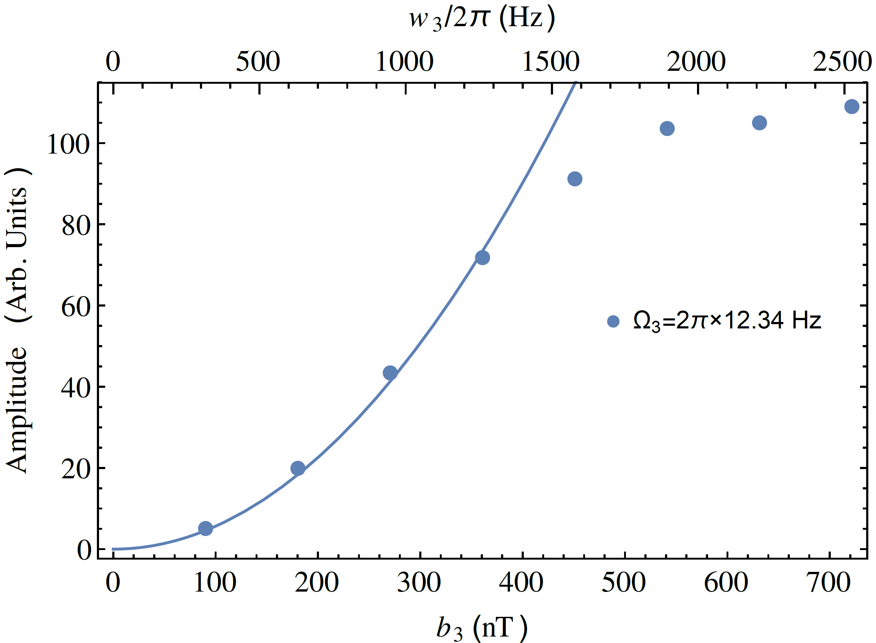
(a)

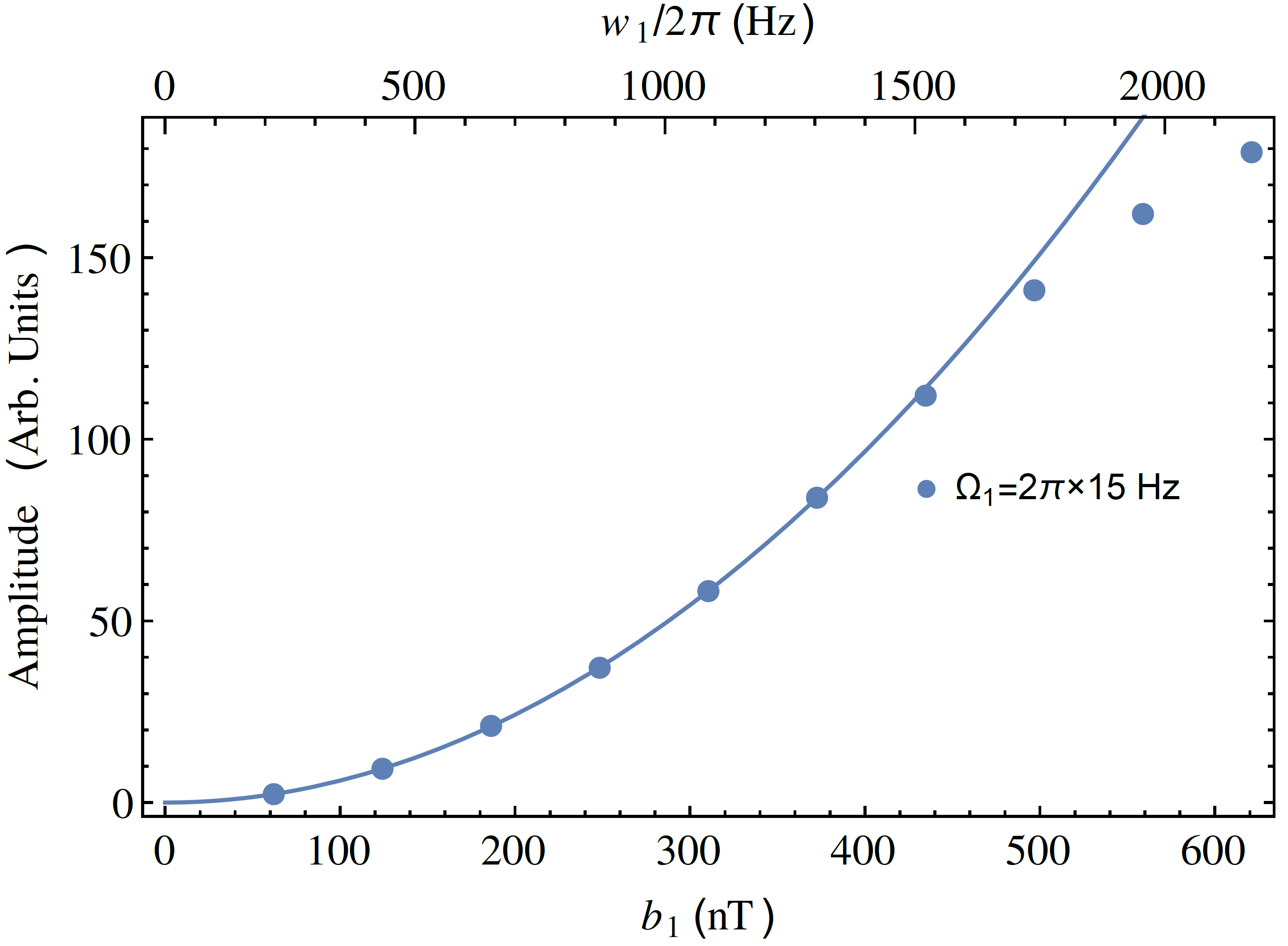
(b)

Figure 5: Quadratic response to the transverse fields. These plots report the second harmonic amplitude registered when an oscillating transverse field is applied. In the case (a) a 12.34 Hz field is applied along $z$ ($b_{3}$, see Eq. 25a), and in the case (b) a 15 Hz field is applied along $x$ ($b_{1}$, see Eq. 25b). A saturation effect appears above 300-400 $\mu$T, while the experimental points recorded at lower field intensity are perfectly fitted by a parabolic curve (solid line). Only the detuning $\delta$ is varied in the best fit procedure, while $\Gamma$ is set a $2\pi$30 Hz. The arbitrary units used for the vertical scales are the same as for the Figs.6 and 7.

When the TDF is applied in the same direction as the bias field, the system second-order response is described by the Eq. 24: the expected amplitude of second-harmonics peak may noticeably vary as a function of $\delta$. In particular, it is expected to vanish for $\delta=0$: a feature that may find application in stabilization systems aimed to maintain the static field correctly oriented and under resonant condition ($\omega_{L}\approx\omega$).

Fig. 6 shows experimental points and a corresponding fitting parabola obtained when a TDF is applied along the bias field with different amplitudes. The fitting curve lets estimate $\delta\approx 50$ rad/s, a value consistent with the experimental conditions.

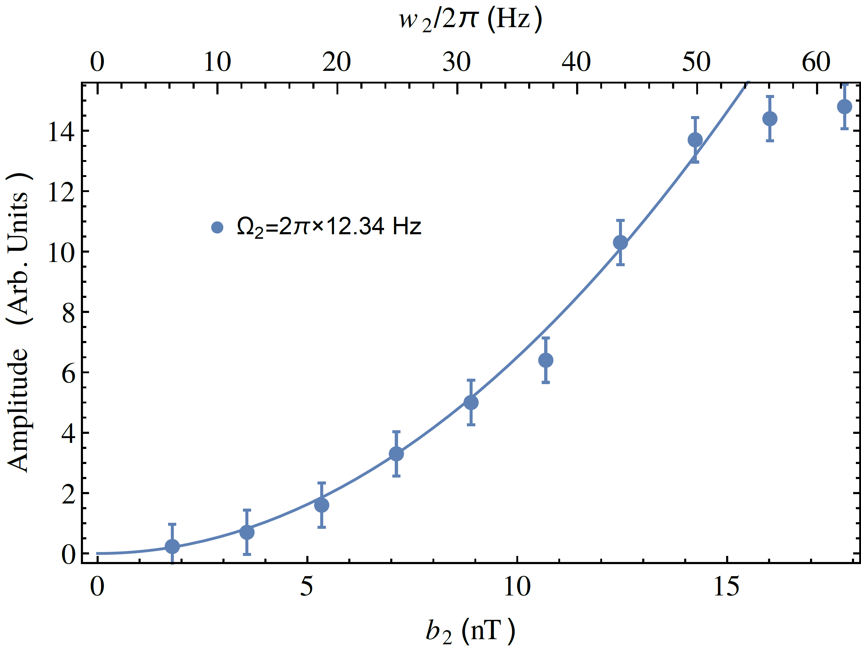
Figure 6: In accordance with Eq. 24, provided that a detuning $\delta$ exists, a second harmonic response with quadratically dependent amplitude is expected, in response to longitudinal TDF. This figure reports the $2\Omega_{2}$ peak registered when a 12.34 Hz oscillating $b_{2}$ field is applied. The relaxation rate is set at $\Gamma=2\pi\cdot 30$ rad/s, and good fitting is found for $\delta=$50 Hz, which is consistent with the experimental conditions. In this case saturation is observed above 15 nT

The Eqs. 26 and 31 describe a linear dependence of the sum- and difference-frequency peaks as a function of either the $x$ or $z$ TDF component. This behaviour is consistent with the data shown in Fig. 7, up to TDF amplitudes around 300 nT. Those data are recorded when applying two sinusoidal TDFs along the $x$ and $z$ directions, at 15 Hz and 12.34 Hz, respectively.

The linear slopes of the fitting curves largely exceed the amount expected from Eq. 26, suggesting that orthogonality imperfections (Eq. 31) play a dominant role in this case. The ratio between the sum- and difference-frequency slopes is approximately 1.4, which is well consistent with the values estimated from Eq. 32 for $\delta\approx 0$ and $\Gamma\approx 2\pi\cdot 30$ Hz.

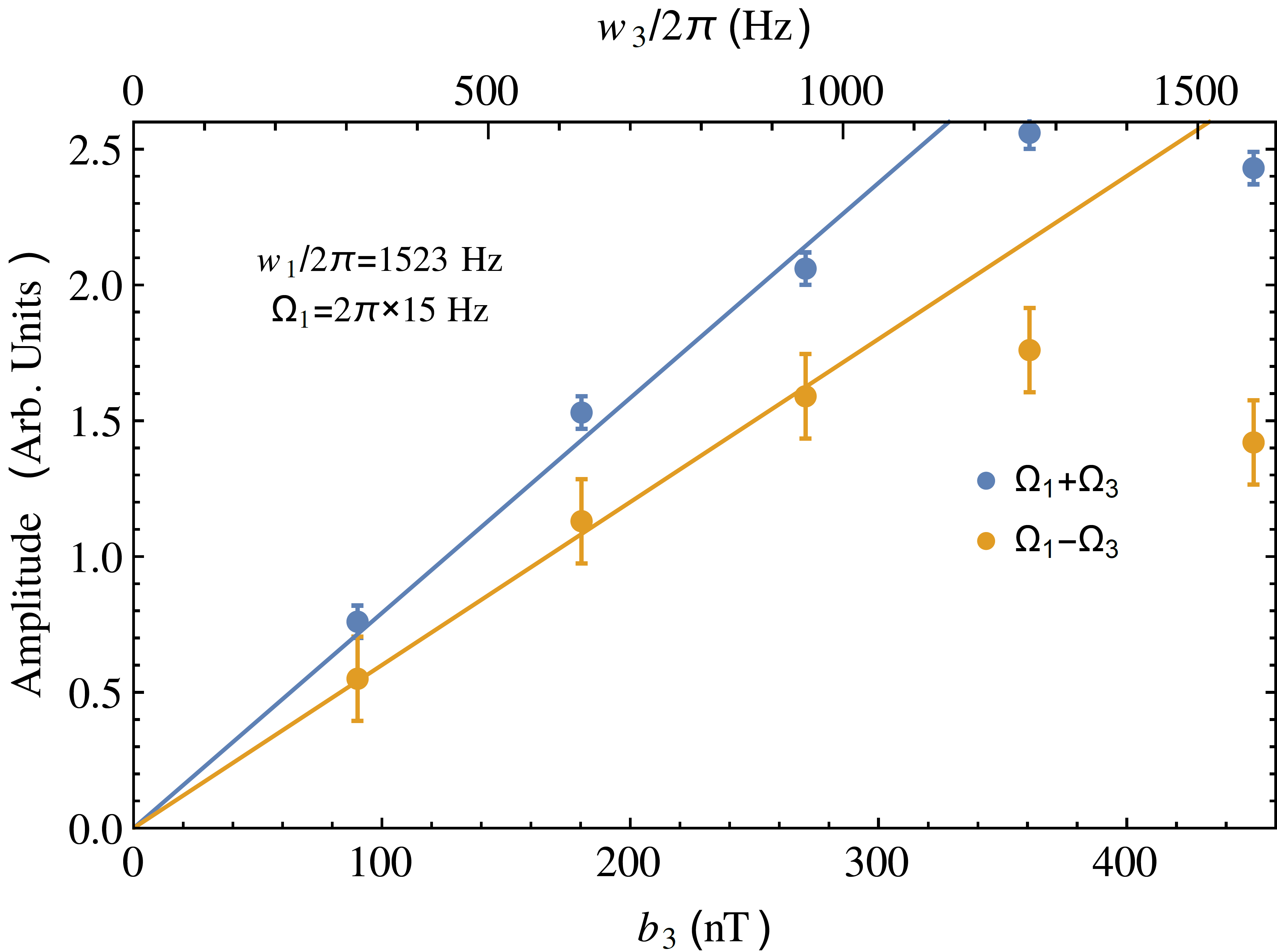
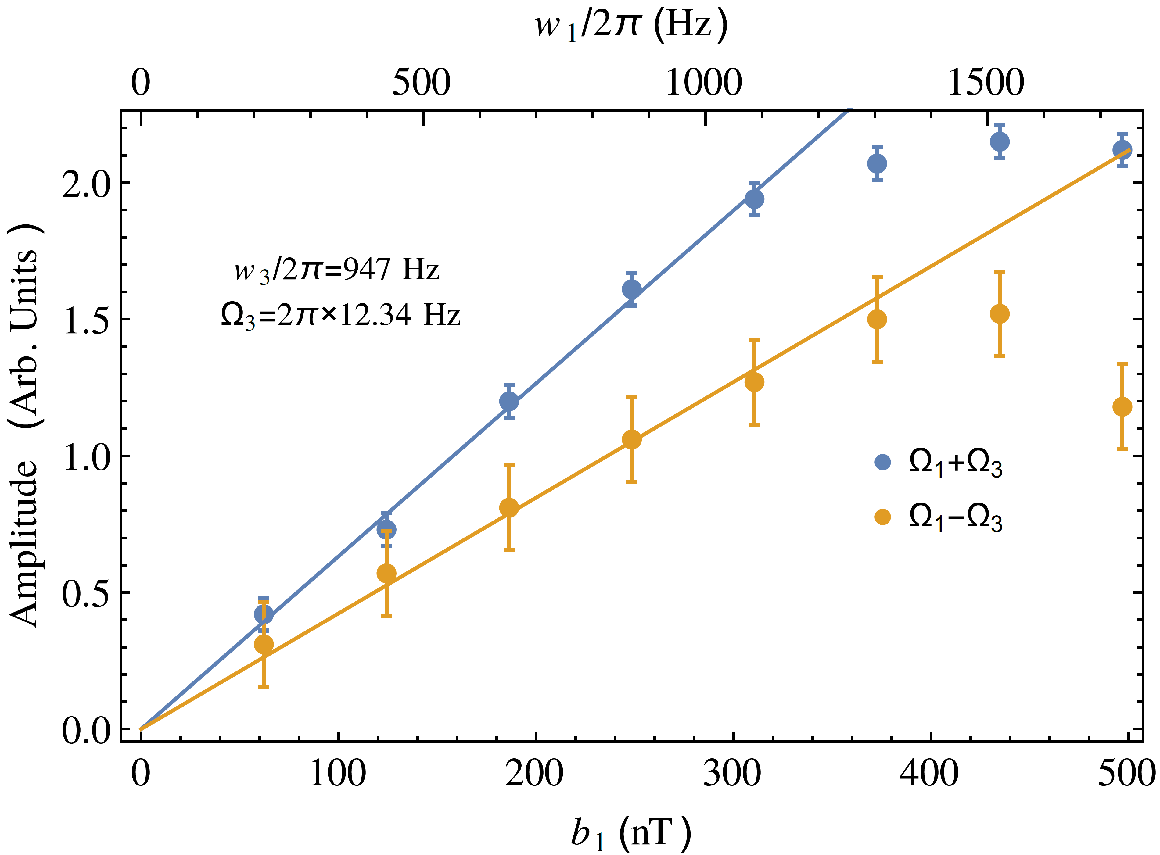
Figure 7: Linear dependence of mixing terms on the $b_{1}$ and $b_{3}$ amplitude. The two plots are obtained when oscillating fields at 15 Hz and 12.34 Hz are simultaneously applied along the $x$ and $z$ directions, respectively. In the upper plot $b_{1}$ is set at 435 nT and $b_{3}$ is varied, while in the lower plot $b_{3}$ is set at 270.6 nT and $b_{1}$ is varied. Peaks at the sum and difference frequencies are recorded. Both the absolute amplitude of the peaks and their ratios indicate that these mixed frequency peaks do not originate from the second order term described in Eq. 26, but are rather caused by imperfect coil orthogonality. The ratio between sum- and difference-frequency peaks is indeed perfectly consistent with the square root of the ratio $R$ expressed in Eq. 32. Similarly to the cases shown in Fig. 5, a saturation effect occurs above about 300 nT.

V Conclusion

We have studied the dynamic response of a parametric system constituted by a light-modulated atomic magnetometer. Such kind of instrumentation is commonly used to detect extremely weak and slowly varying fields. Under these conditions, these devices are often analyzed with an implicit assumption, leading to treat them in analogy with linear time-invariant systems. We have developed a model that provides a more detailed analysis, and particularly let determine the response to TDFs that can range in a wider frequency interval and may have larger amplitudes.

In a first order approximation, which is valid for tiny TDF, we find that the system responds only to the TDF component along the bias field, and that it acts as a low-pass or a band-pass filter, in dependence of the frequency mismatch between the Larmor precession and the pump laser modulation signal. Conditions to achieve maximally flat spectral response, or frequency independent dephasing are identified.

Extending the model to the second order approximation permits to analyze the system behaviour when larger TDFs are applied. Our findings show that the system responds quadratically to both longitudinal and transverse TDF components. The model provides quantitative evaluations of the diverse coefficients that describe amplitudes and phases of those nonlinear terms. In addition, frequency mixing may emerge between harmonic TDF components applied along the two transverse directions. The mixing occurs at different levels, depending on the relative orientation of the oscillating fields. In application (particularly when high resolution magnetometry is performed in the presence of narrow-band disturbances), this analysis will help to identify the origin of spurious spectral peaks that constitute artefacts in the detected signals.

References

- (1) H. G. Dehmelt, “Modulation of a light beam by precessing absorbing atoms,” Phys. Rev., vol. 105, pp. 1924–1925, Mar 1957.
- (2) W. E. Bell and A. L. Bloom, “Optical detection of magnetic resonance in alkali metal vapor,” Phys. Rev., vol. 107, pp. 1559–1565, Sep 1957.
- (3) W. E. Bell and A. L. Bloom, “Optically driven spin precession,” Phys. Rev. Lett., vol. 6, pp. 280–281, Mar 1961.
- (4) Dupont-Roc, J., “Détermination par des méthodes optiques des trois composantes d’un champ magnétique très faible,” Rev. Phys. Appl. (Paris), vol. 5, no. 6, pp. 853–864, 1970.
- (5) J. Dupont-Roc, S. Haroche, and C. Cohen-Tannoudji, “Detection of very weak magnetic fields (gauss) by 87Rb zero-field level crossing resonances,” Physics Letters A, vol. 28, no. 9, pp. 638 – 639, 1969.
- (6) M. Faraday, “I. Experimental researches in electricity.— Nineteenth series,” Philos. Trans. R. Soc. London, vol. 136, 1846.
- (7) D. Macaluso and O. M. Corbino, “Sopra Una Nuova Azione Che La Luce Subisce Attraversando Alcuni Vapori Metallici In Un Campo Magnetico,” Nuovo Cimento, vol. 8, p. 257, 1898.
- (8) D. Macaluso and O. M. Corbino, “Sulla Relazione Tra Il Fenomeno Di Zeemann E La Rotazione Magnetica Anomala Del Piano Di Polarizzazione Della Luce,” Nuovo Cimento, vol. 9, p. 384, 1899.
- (9) W. Happer, “Optical pumping,” Rev. Mod. Phys., vol. 44, pp. 169–249, Apr 1972.
- (10) W. Happer, Y. Jau, and T. Walker, Optical Pumping of Atoms, ch. 5, pp. 49–71. John Wiley & Sons, Ltd, 2010.
- (11) E. Alexandrov, M. Balabas, A. Pasgalev, A. Vershovskii, and N. Yakobson, “Double-resonance atomic magnetometers: From gas discharge to laser pumping,” Laser Physics, vol. 6, no. 2, pp. 244–251, 1996.
- (12) D. Budker and M. Romalis, “Optical magnetometry,” Nature Physics, vol. 3, pp. 227–234, 2007.
- (13) I. Savukov, “Ultra-sensitive optical atomic magnetometers and their applications,” in Advances in Optical and Photonic Devices (K. Y. Kim, ed.), ch. 17, Rijeka: IntechOpen, 2010.
- (14) C. M. Swank, E. K. Webb, X. Liu, and B. W. Filippone, “Spin-dressed relaxation and frequency shifts from field imperfections,” Phys. Rev. A, vol. 98, p. 053414, Nov 2018.
- (15) V. Guarrera, R. Gartman, G. Bevilacqua, G. Barontini, and W. Chalupczak, “Parametric amplification and noise squeezing in room temperature atomic vapors,” Phys. Rev. Lett., vol. 123, p. 033601, Jul 2019.
- (16) C. Abel, S. Afach, N. J. Ayres, G. Ban, G. Bison, K. Bodek, V. Bondar, E. Chanel, P.-J. Chiu, C. B. Crawford, Z. Chowdhuri, M. Daum, S. Emmenegger, L. Ferraris-Bouchez, M. Fertl, B. Franke, W. C. Griffith, Z. D. Grujić, L. Hayen, V. Hélaine, N. Hild, M. Kasprzak, Y. Kermaidic, K. Kirch, P. Knowles, H.-C. Koch, S. Komposch, P. A. Koss, A. Kozela, J. Krempel, B. Lauss, T. Lefort, Y. Lemière, A. Leredde, A. Mtchedlishvili, P. Mohanmurthy, M. Musgrave, O. Naviliat-Cuncic, D. Pais, A. Pazgalev, F. M. Piegsa, E. Pierre, G. Pignol, P. N. Prashanth, G. Quéméner, M. Rawlik, D. Rebreyend, D. Ries, S. Roccia, D. Rozpedzik, P. Schmidt-Wellenburg, A. Schnabel, N. Severijns, R. T. Dinani, J. Thorne, A. Weis, E. Wursten, G. Wyszynski, J. Zejma, and G. Zsigmond, “Optically pumped cs magnetometers enabling a high-sensitivity search for the neutron electric dipole moment,” Phys. Rev. A, vol. 101, p. 053419, May 2020.
- (17) H. Korth, K. Strohbehn, F. Tejada, A. G. Andreou, J. Kitching, S. Knappe, S. J. Lehtonen, S. M. London, and M. Kafel, “Miniature atomic scalar magnetometer for space based on the rubidium isotope 87Rb,” Journal of Geophysical Research: Space Physics, vol. 121, no. 8, pp. 7870–7880, 2016.
- (18) A. Pollinger, R. Lammegger, W. Magnes, C. Hagen, M. Ellmeier, I. Jernej, M. Leichtfried, C. Kürbisch, R. Maierhofer, R. Wallner, G. Fremuth, C. Amtmann, A. Betzler, M. Delva, G. Prattes, and W. Baumjohann, “Coupled dark state magnetometer for the china seismo-electromagnetic satellite,” Measurement Science and Technology, vol. 29, p. 095103, aug 2018.
- (19) M. D. Prouty, R. Johnson, I. Hrvoic, and A. K. Vershovskiy, Geophysical applications, p. 319–336. Cambridge University Press, 2013.
- (20) J. W. E. Fassbinder, Magnetometry for Archaeology, pp. 499–514. Dordrecht: Springer Netherlands, 2017.
- (21) V. Mathé, L. François, and M. Druez, “What interest to use caesium magnetometer instead of fluxgate gradiometer?,” ArcheoSciences, vol. 33, pp. 325–327, 2009.
- (22) A. Jaufenthaler, P. Schier, T. Middelmann, M. Liebl, F. Wiekhorst, and D. Baumgarten, “Quantitative 2D magnetorelaxometry imaging of magnetic nanoparticles using optically pumped magnetometers,” Sensors, vol. 20, no. 3, 2020.
- (23) L. Marmugi, C. Deans, and F. Renzoni, “Electromagnetic induction imaging with atomic magnetometers: Unlocking the low-conductivity regime,” Applied Physics Letters, vol. 115, no. 8, p. 083503, 2019.
- (24) K. Jensen, M. Zugenmaier, J. Arnbak, H. Stærkind, M. V. Balabas, and E. S. Polzik, “Detection of low-conductivity objects using eddy current measurements with an optical magnetometer,” Phys. Rev. Research, vol. 1, p. 033087, Nov 2019.
- (25) P. Bevington, R. Gartman, and W. Chalupczak, “Enhanced material defect imaging with a radio-frequency atomic magnetometer,” Journal of Applied Physics, vol. 125, no. 9, p. 094503, 2019.
- (26) H. Xia, A. Ben-Amar Baranga, D. Hoffman, and M. V. Romalis, “Magnetoencephalography with an atomic magnetometer,” Applied Physics Letters, vol. 89, no. 21, p. 211104, 2006.
- (27) I. M. Savukov and M. V. Romalis, “NMR detection with an atomic magnetometer,” Phys. Rev. Lett., vol. 94, p. 123001, Mar 2005.
- (28) G. Bevilacqua, V. Biancalana, Y. Dancheva, A. Vigilante, A. Donati, and C. Rossi, “Simultaneous detection of H and D NMR signals in a micro-Tesla field,” The Journal of Physical Chemistry Letters, vol. 8, pp. 6176–6179, 2017. PMID: 29211488.
- (29) M. C. Tayler and L. F. Gladden, “Scalar relaxation of NMR transitions at ultralow magnetic field,” Journal of Magnetic Resonance, vol. 298, pp. 101–106, 2019.
- (30) G. Bevilacqua, V. Biancalana, Y. Dancheva, and A. Vigilante, “Sub-millimetric ultra-low-field MRI detected in situ by a dressed atomic magnetometer,,” Appl.Phys.Lett., vol. 115, p. 174102, 2019.
- (31) J. W. Blanchard, T. Wu, J. Eills, Y. Hu, and D. Budker, “Zero- to ultralow-field nuclear magnetic resonance J-spectroscopy with commercial atomic magnetometers,” Journal of Magnetic Resonance, vol. 314, p. 106723, 2020.
- (32) S. Xu, V. V. Yashchuk, M. H. Donaldson, S. M. Rochester, D. Budker, and A. Pines, “Magnetic resonance imaging with an optical atomic magnetometer,” Proceedings of the National Academy of Sciences, vol. 103, no. 34, pp. 12668–12671, 2006.
- (33) N. Wilson, C. Perrella, R. Anderson, A. Luiten, and P. Light, “Wide-bandwidth atomic magnetometry via instantaneous-phase retrieval,” Phys. Rev. Research, vol. 2, p. 013213, Feb 2020.
- (34) K. Jensen, M. A. Skarsfeldt, H. Stærkind, J. Arnbak, M. V. Balabas, S.-P. Olesen, B. H. Bentzen, and E. S. Polzik, “Magnetocardiography on an isolated animal heart with a room-temperature optically pumped magnetometer,” Scientific Reports, vol. 8, p. 16218, 2018.
- (35) S. J. Ingleby, C. O’Dwyer, P. F. Griffin, A. S. Arnold, and E. Riis, “Orientational effects on the amplitude and phase of polarimeter signals in double-resonance atomic magnetometry,” Phys. Rev. A, vol. 96, p. 013429, Jul 2017.
- (36) I. Savukov, Y. J. Kim, V. Shah, and M. G. Boshier, “High-sensitivity operation of single-beam optically pumped magnetometer in a kHz frequency range,” Measurement Science and Technology, vol. 28, p. 035104, feb 2017.
- (37) L. G. Villanueva, R. B. Karabalin, M. H. Matheny, E. Kenig, M. C. Cross, and M. L. Roukes, “A nanoscale parametric feedback oscillator,” Nano Letters, vol. 11, no. 11, pp. 5054–5059, 2011. PMID: 22007833.
- (38) Z. C. Feng and K. Gore, “Dynamic characteristics of vibratory gyroscopes,” IEEE Sensors Journal, vol. 4, no. 1, pp. 80–84, 2004.
- (39) K. Santhosh and B. Roy, “A smart displacement measuring technique using linear variable displacement transducer,” Procedia Technology, vol. 4, pp. 854 – 861, 2012. 2nd International Conference on Computer, Communication, Control and Information Technology( C3IT-2012) on February 25 - 26, 2012.
- (40) S. Surappa, S. Satir, and F. Levent Degertekin, “A capacitive ultrasonic transducer based on parametric resonance,” Applied physics letters, vol. 111, p. 043503, July 2017.
- (41) Z. Ding, J. Yuan, and L. X, “Response of a Bell-Bloom magnetometer to a magnetic field of arbitrary direction,” Sensors, vol. 18, p. 1401, May 2018.
- (42) G. Bevilacqua, V. Biancalana, P. Chessa, and Y. Dancheva, “Multichannel optical atomic magnetometer operating in unshielded environment,” Applied Physics B, vol. 122, no. 4, p. 103, 2016.
- (43) R. Zhang, T. Wu, J. Chen, X. Peng, and H. Guo, “Frequency response of optically pumped magnetometer with nonlinear Zeeman effect,” Applied Sciences, vol. 10, no. 20, 2020.
- (44) J. M. Higbie, E. Corsini, and D. Budker, “Robust, high-speed, all-optical atomic magnetometer,” Review of Scientific Instruments, vol. 77, no. 11, p. 113106, 2006.
- (45) J. Belfi, G. Bevilacqua, V. Biancalana, S. Cartaleva, Y. Dancheva, K. Khanbekyan, and L. Moi, “Dual channel self-oscillating optical magnetometer,” J. Opt. Soc. Am. B, vol. 26, pp. 910–916, May 2009.
- (46) G. Bevilacqua, V. Biancalana, Y. Dancheva, and L. Moi, “Larmor frequency dressing by a nonharmonic transverse magnetic field,” Phys. Rev. A, vol. 85, p. 042510, Apr 2012.
- (47) G. Bevilacqua, V. Biancalana, Y. Dancheva, and A. Vigilante, “Restoring narrow linewidth to a gradient-broadened magnetic resonance by inhomogeneous dressing,” Phys. Rev. Applied, vol. 11, p. 024049, Feb 2019.
- (48) A. P. Colombo, T. R. Carter, A. Borna, Y.-Y. Jau, C. N. Johnson, A. L. Dagel, and P. D. D. Schwindt, “Four-channel optically pumped atomic magnetometer for magnetoencephalography,” Opt. Express, vol. 24, pp. 15403–15416, Jul 2016.
- (49) R. Zhang, B. Pang, W. Li, Y. Yang, J. Chen, X. Peng, and H. Guo, “Frequency response of a close-loop Bell-Bloom magnetometer,” in 2018 IEEE International Frequency Control Symposium (IFCS), pp. 1–3, 2018.
- (50) G. Bevilacqua, V. Biancalana, Y. Dancheva, and A. Vigilante, “Self-adaptive loop for external-disturbance reduction in a differential measurement setup,” Phys. Rev. Applied, vol. 11, p. 014029, Jan 2019.
- (51) R. Zhang, Y. Ding, Y. Yang, Z. Zheng, J. Chen, X. Peng, T. Wu, and H. Guo, “Active magnetic-field stabilization with atomic magnetometer,” Sensors, vol. 20, no. 15, 2020.
- (52) G. Bevilacqua, V. Biancalana, A. Ben Amar Baranga, Y. Dancheva, and C. Rossi, “Micro-Tesla NMR J-coupling spectroscopy with an unshielded atomic magnetometer,” Journal of Magnetic Resonance, vol. 263, pp. 65–70, 2016.