Ground state features and spectral properties of large polaron liquids from low to high charge densities

Abstract

A new variational approach is proposed at zero temperature for a finite density of charge carriers in order to study ground state features of the Fröhlich model including electron-electron and electron-phonon interactions. Within the intermediate electron-phonon coupling regime characteristic of large polarons, the approach takes into account on the same footing polaron formation and polaron-polaron correlations which play a relevant role going from low to high charge densities. Including fluctuations on top of the variational approach, the electronic spectral function is calculated from the weak to the intermediate electron-phonon coupling regime finding a peak-dip-hump line shape. The spectra are characterized by a transfer of spectral weight from the incoherent hump to the coherent peak with decreasing the electron-phonon coupling constant or with increasing the particle density. Three different density regimes stem out: the first, at low densities, where the features of a single large polaron with a substantial incoherent spectral weight are not modified by charge carrier interactions; a second one, at intermediate densities, where the polaronic liquid shows a rapid crossover from incoherent to coherent dynamics; the third one, at high densities, where screening effects are so prominent that the system presents a conventional metallic phase. The results obtained in the low to intermediate density regime turn out to be relevant for the interpretation of recent tunneling and photoemission experiments in $SrTiO_{3}$-based systems.

I introduction

The polaron is a fermionic quasiparticle which takes into account the interaction of an electron with lattice vibrations in a solid [1, 2, 3]. This concept has been originally used in polar semiconductors to indicate that the polarization cloud follows the electron in its motion. Indeed, a first classification of the polaron is based on the size of the phonon cloud. If the electron-phonon coupling is not very strong, the phonon cloud accompanying the electron extends over lengths larger than the lattice parameter of the solid, therefore the corresponding polaron is termed large. Large polarons are itinerant quasi-particles whose dynamics affects the spectral, transport and optical properties of solids.

In the last years $SrTiO_{3}$-based (STO) systems have become one of the main research areas of the condensed matter community [4, 5]. Not only the three-dimensional (3D) STO bulk but also the two-dimensional (2D) STO surface and quasi-2D heterostuctures, such as those between STO and $LaAlO_{3}$ (LAO), have been much studied showing many interesting properties among which superconducting phases strongly tunable by chemical doping (in the bulk) or by application of a gate potential (in the heterostructures). In particular, at odds with simple metallic systems, superconducting states occur at quite low carrier densities [6, 7] suggesting the presence of large pairing potentials and novel features of the normal state. In order to interpret the bulk data from angle-resolved photoemission spectroscopy (ARPES) [8, 9, 10, 11], it has been suggested that a substantial interaction between electrons and lattice distortions plays a significant role. The relevance of large polaron quasi-particles [12] has been confirmed by the experimental spectral properties not only of the 3D bulk [13], but also the 2D surface [14, 15] and LAO/STO heterostructure [16]. In particular, the large polaron formation is promoted by the sizable coupling of the electron with a well-defined high frequency longitudinal optical mode [13, 14, 16]. In addition to tunneling and photoemission spectra, the optical properties [17, 18] and inelastic x-ray scattering measurements [19] have shown that the charge carriers undergo a crossover from a polaronic liquid to a Fermi liquid regime with increasing density. Nowadays the role of large polarons is widely recognized in STO-based materials.

The Fröhlich model has been frequently used to simulate the large polaron formation when the relevant coupling is between electrons and longitudinal optical phonons in polar materials [1, 2, 3, 20]. In STO-based systems, experimental data have been interpreted within the Fröhlich model [12] suggesting that the electron-phonon interaction is not perturbative, but in the intermediate coupling regime. For the single Fröhlich polaron, the different coupling regimes of the electron-phonon interaction have been investigated by several variational approaches [2, 20, 21] which provide also the starting point for excited state properties [22]. A simple variational approach is that based on the Lee-Low-Pines (LLP) canonical transformation which is quite accurate in the weak to intermediate electron-phonon coupling regime [23, 24]. All the results of these variational approaches for the single polaron have been checked by many numerical methods, among which that based on the diagrammatic quantum Monte Carlo (DQMC) [12, 25] is one of the most accurate for all the electron-phonon couplings.

Theory for many polaron systems is feasible for weak electron-phonon couplings [3, 13, 14], but it is quite challenging for non-perturbative regimes [12, 26, 27, 28]. Considering only the effects of the electron-phonon interaction, a recent theoretical study has shown that the crossover from polarons to Fermi liquids in transition metal oxides, among which titanates, occurs when the frequency of plasma oscillations exceeds that of longitudinal optical phonons [29]. For STO-based systems, the optical response has been calculated starting from the Fröhlich model including Coulomb electron-electron interactions [30, 31]. However, many features of the full Fröhlich model, such as the spectral properties, are not fully understood in the intermediate electron-phonon coupling regime. One possibility to approach this problem is to generalize the variational approaches for the single polaron to the many particle case [1]. Indeed, the LLP canonical transformation has been performed in second quantization to treat variationally the electron-phonon interaction for a finite density of charge carriers [32]. One drawback of these approaches is that, after the canonical transformation to the polaron configuration space, polaron-polaron interactions have been treated only at Hartree-Fock level. It is highly desirable to treat the electron liquid with polaronic effects beyond the mean-field theory [33].

In this paper, in order to analyze the ground state properties of the Fröhlich model in the intermediate electron-phonon coupling regime, we explicitly include polaron-polaron correlations after the variational many-particle LLP canonical transformation. Actually, polaron-polaron interactions are taken into account through a variational Slater-Jastrow term in the many-body wave-function which, therefore, includes the suppression of long wavelength density fuctuations [34]. In fact, the treatment of charge correlations is at the same level of the many-body approach known as Random Phase Approximation (RPA) [3]. Many quantities, such as the static structure factor and the polaronic band shift, have been evaluated pointing out that polaron-polaron correlations represent very relevant effects with increasing particle density.

The electronic spectral function is calculated from the weak to the intermediate electron-phonon coupling regime for different carrier concentrations by including fluctuations on top of the variational approach. The large polaron spectra are characterized by a peak-dip-hump line shape. For the single polaron, in the intermediate electron-phonon coupling regime, the hump has a relevant spectral weight and it consists of several phonon satellites in good agreement with numerical approaches. Screening promotes a transfer of spectral weight from the incoherent hump to the coherent peak with increasing the particle density. In agreement with recent tunneling and photoemission experiments in STO-based systems [13, 14, 16], we identify three different density regimes: the low density one, where the spectra bear a strong resemblance to those of the single large polaron; the intermediate density one, where the crossover from incoherent to coherent dynamics is quite rapid; the high density one, where the system behaves as a conventional metal. It turns out that the role of density can be roughly understood as an effect leading to the reduction of the effective electron-phonon coupling constant. However, for intermediate electron-phonon couplings, the density evolution of the spectral properties can not be ascribed only to many-body screening, but also to polaron features ranging from the antiadiabatic to the adiabatic regime. Our results are fully consistent with experimental findings in STO-based systems clarifying the role of the electron-phonon coupling in the low to intermediate density regime.

The paper is organized as follows. In section II the model and the variational approach are reviewed; in section III the spectral properties are discussed; in section IV conclusions and discussions. We present additional details about polaron-phonon couplings in Appendix A, and polaronic spectral features in Appendix B.

II The model and the variational approach

In this paper, the Fröhlich model [3, 23] is studied focusing on the normal state of $N$ polarons at zero temperature. The starting point of the model is the jellium for interacting electrons. In addition to the Coulomb electron-electron interaction, the model takes into account the coupling between electrons and longitudinal optical phonons. The long-range electron-phonon interaction is derived under the assumption that the medium is a polarizable continuum with partially ionic character. The Fröhlich model has been extensively used for the description of doped polar semiconductors [3].

The Hamiltonian $H$ of the Fröhlich model in second quantization is the following:

$$H=H_{el}^{(0)}+H_{ph}^{(0)}+H_{el-el}^{\infty}+H_{el-ph},$$ (1)

where the first term $H_{el}^{(0)}$, defined as

$$H_{el}^{(0)}=\sum_{{\bf k},\sigma}\frac{\hbar^{2}k^{2}}{2m}c^{\dagger}_{{\bf k},\sigma}c_{{\bf k},\sigma},$$ (2)

describes the conduction band electrons of wave-vector ${\bf k}$ ($k=|{\bf k}|$ its modulus), mass $m$ and spin $\sigma$, with $c^{\dagger}_{{\bf k},\sigma}\left(c_{{\bf k},\sigma}\right)$ the related creation (annihilation) operator, while the second term $H_{ph}^{(0)}$, defined as

$$H_{ph}^{(0)}=\hbar\omega_{LO}\sum_{{\bf q}}a^{\dagger}_{{\bf q}}a_{{\bf q}},$$ (3)

characterizes the energy of free longitudinal optical phonons of wave-vector ${\bf q}$ and angular frequency $\omega_{LO}$, with $a^{\dagger}_{{\bf q}}\left(a_{{\bf q}}\right)$ related creation (annihilation) phonon operator.

In Eq. (1), the electron-electron interaction is provided by the following Hamiltonian $H_{el-el}^{\infty}$

$$H_{el-el}^{\infty}=\frac{1}{2V}\sum_{{\bf q}}V_{q}^{\infty}\left(\rho_{\bf q}\rho^{\dagger}_{\bf q}-N\right),$$ (4)

where $V$ is the volume of the system, $\rho_{q}$ is the density operator

$$\rho_{\bf q}=\sum_{{\bf k},\sigma}c^{\dagger}_{{\bf k}+{\bf q},\sigma}c_{{\bf k},\sigma},$$ (5)

and $V_{q}^{\infty}$ is the Coulomb potential

$$V_{q}^{\infty}=\frac{4\pi e^{2}}{\epsilon_{\infty}q^{2}},$$ (6)

with $e$ the modulus of the electron charge, $\epsilon_{\infty}$ the dielectric function at frequencies higher than those of the optical modes, $\hbar q$ the modulus of the momentum exchanged by the electrons. Actually, the dielectric constant $\epsilon_{\infty}$ takes into account electronic excitations across the semiconductor gap, which are therefore at high energies. Indeed, these electronic excitations provide a constant contribution on the low energy scale of vibrational modes and conduction electrons close to the Fermi energy.

In Eq. (1), the electron-phonon interaction is given by the following Hamiltonian $H_{el-ph}$

$$H_{el-ph}=\frac{1}{\sqrt{V}}\sum_{{\bf q}}M_{q}\rho_{{\bf q}}\left(a_{{\bf q}}+a^{\dagger}_{-{\bf q}}\right),$$ (7)

where the electron-phonon matrix element $M_{q}$ is

$$M_{q}=\hbar\omega_{LO}\frac{\sqrt{4\pi\alpha R_{p}}}{q}.$$ (8)

In Eq. (8), the dimensionless electron-phonon coupling constant $\alpha$, defined as

$$\alpha=\frac{e^{2}}{2R_{p}\hbar\omega_{LO}}\left(\frac{1}{\epsilon_{\infty}}-\frac{1}{\epsilon_{0}}\right),$$ (9)

is determined not only by $\epsilon_{\infty}$, but also by the static dielectric constant $\epsilon_{0}$, therefore it depends on the polarizability of the system. Moreover, $R_{p}$ is the polaron radius defined as

$$R_{p}=\sqrt{\frac{\hbar}{2m\omega_{LO}}}.$$ (10)

The parameters of the many-body Hamiltonian (1) are the electron mass $m$, the phonon angular frequency $\omega_{LO}$, the dielectric constants $\epsilon_{\infty}$ and $\epsilon_{0}$. Another important quantity in this paper is the particle density $n=N/V$, which determines the Fermi wave-vector $k_{F}$. In the case of STO-based systems, the following values are assumed [5, 30, 35]: $m\simeq 2m_{0}$, with $m_{0}$ electron rest mass, $\omega_{LO}\simeq 2.42\cdot 10^{13}s^{-1}$ (corresponding to $\hbar\omega_{LO}\simeq 100$ meV), $\epsilon_{\infty}\simeq 5.1$, and $\epsilon_{0}\simeq 2\cdot 10^{4}$. This high frequency phonon mode is the most coupled to the electrons and it is clearly discernible in experimental measurements [15, 14, 16]. We remark that a model with a single electronic band does not represent a limitation for the analysis of STO-based systems, since, in the ARPES setup, it is possible to use polarized light in order to investigate selected electronic bands. For example, using s-polarized light [14], the measurements can resolve a single $d_{xy}$ band at low density.

By using the Hamiltonian parameters and Eq. (9), one gets the electron-phonon coupling constant $\alpha\simeq 3.37$, that is STO-based systems are well within the intermediate electron-phonon coupling regime. This non-perturbative coupling regime is notoriously difficult to analyze in systems, like STO-based compounds, whose static and dynamic properties are sensitive to the variations of particle density. Indeed, an important feature of STO-based systems is the possibility to tune the particle density over several orders of magnitude. In the next subsection, we expose our new variational approach which takes into account both the polaron formation and the effects of polaron-polaron interactions from weak to intermediate electron-phonon coupling regime ranging from low to high densities.

II.1 Variational approach

Following a proposed variational scheme valid for a finite number $N$ of electrons [32], the LLP canonical transformation [23] is performed in second quantization to treat variationally the electron-phonon interaction up to the intermediate coupling regime ($\alpha<6$). The variational unitary transformation $U$ is

$$U=\exp\left[\frac{1}{\sqrt{V}}\sum_{{\bf q}}f_{q}\rho_{{\bf q}}\left(a_{{\bf q}}-a^{\dagger}_{-{\bf q}}\right)\right],$$ (11)

where $f_{q}$ is a real variational function, which provides the phonon distribution function induced by the electron dynamics. Actually, the function $f_{q}$ shifts the position of the vibrational modes quantifying the strength of the coupling between electron and lattice displacement, hence it measures the degree of polaronic effect. We point out that, even in the intermediate electron-phonon coupling regime, the interactions at zero temperature are not able to localize the electron, that this way behaves as an itinerant large polaron [1, 2, 20].

The transformed Hamiltonian $\tilde{H}=U^{-1}HU$ describes the interaction between large polarons and shifted vibrational modes being

$$\tilde{H}=H_{ph}^{(0)}+H_{pol}+H_{pol-ph}+H_{pol-2ph},$$ (12)

where $H_{ph}^{(0)}$ is the free phonon Hamiltonian equal to Eq. (3), and $H_{pol}$ describes many interacting large polarons:

$$H_{pol}=H_{pol}^{(0)}+H_{pol-pol}.$$ (13)

In Eq. (13), the free polaron Hamiltonian $H_{pol}^{(0)}$ has the same form as the kinetic energy in Eq. (2), but the quadratic term in the momentum is replaced by the polaronic band $\epsilon_{k}$

$$\epsilon_{k}=\frac{\hbar^{2}k^{2}}{2m}+\eta,$$ (14)

with the polaronic band shift $\eta$ given by

$$\eta=\frac{1}{V}\sum_{{\bf q}}\left(\hbar\omega_{LO}+\frac{\hbar^{2}q^{2}}{2m}\right)f^{2}_{q}-\frac{2}{V}\sum_{{\bf q}}M_{q}f_{q}.$$ (15)

In Eq. (13), the polaron-polaron interaction term $H_{pol-pol}$ has the same form as Eq. (4), with $V_{q}^{\infty}$ replaced by the following effective potential $V_{q}^{eff}$:

$$V_{q}^{eff}=V_{q}^{\infty}+2\left(\hbar\omega_{LO}f^{2}_{q}-2M_{q}f_{q}\right).$$ (16)

Due to the electron-phonon interaction, the effective potential gets reduced in comparison with the bare repulsive one. Moreover, in the strong electron-phonon coupling regime ($\alpha>6$, not analyzed in this paper), $V_{q}^{eff}$ can also present a negative sign for some values of the wave-vector $q$ (characteristic of an attractive interaction), thus favoring the stability of bipolaronic [36] or charge-ordered phases [27] different from the normal state considered in this paper. Therefore, the unitary transformation $U$ given in Eq. (11) takes into account very relevant effects due to the electron-phonon coupling, that is both the band shift in Eq. (15) and the effective polaron-polaron potential in Eq. (16), which in fact depend on the phonon distribution function $f_{q}$. Other renormalization effects can be determined analyzing the role played by further interaction terms of the transformed Hamiltonian $\tilde{H}$.

In Eq. (12), the residual polaron-phonon interaction term $H_{pol-ph}$ consists of two contributions:

$$H_{pol-ph}=H_{pol-ph}^{(1)}+H_{pol-ph}^{(2)},$$ (17)

where $H_{pol-ph}^{(1)}$ has the same form as Eq. (7), with $M_{q}$ replaced by the following effective matrix element $M_{q}^{eff}$

$$M_{q}^{eff}=M_{q}-\hbar\omega_{LO}f_{q},$$ (18)

therefore, as expected, the resulting polaron-phonon vertex is reduced in comparison with the bare electron-phonon one. In Eq. (17), $H_{pol-ph}^{(2)}$ is more complex being

$$H_{pol-ph}^{(2)}=\frac{1}{\sqrt{V}}\sum_{{\bf k},{\bf q},\sigma}N_{{\bf k},{\bf k}+{\bf q}}c^{\dagger}_{{\bf k}+{\bf q},\sigma}c_{{\bf k},\sigma}\left(a_{{\bf q}}-a^{\dagger}_{-{\bf q}}\right),$$ (19)

where the electron-phonon matrix element $N_{{\bf k},{\bf k}+{\bf q}}$ is

$$N_{{\bf k},{\bf k}+{\bf q}}=\frac{\hbar^{2}f_{q}}{2m}{\bf q}\cdot({\bf q}+2{\bf k})=\frac{\hbar^{2}f_{q}}{2m}({\bf k}+{\bf q}-{\bf k})\cdot({\bf k}+{\bf q}+{\bf k}).$$ (20)

Actually, $H_{pol-ph}^{(2)}$ derives from the unitary transformation of the kinetic energy in Eq. (2), and it is not a function of the position operator but of the momentum operator of phonons. Moreover, the polaron-phonon vertex in $H_{pol-ph}^{(2)}$ does not simply depend on the phonon momentum ${\bf q}$, but it is a function of the incoming vector ${\bf k}$ and the outgoing vector ${\bf k}+{\bf q}$. In the following sections, we will find that the effects due to the term $H_{pol-ph}^{(2)}$ on the spectral properties of large polarons in the intermediate coupling regime are not negligible in comparison with those due to the term $H_{pol-ph}^{(1)}$ when the charge density is low.

Finally, in Eq. (12), the polaron-two phonon interaction term $H_{pol-2ph}$ describes the interaction between phonons mediated by polarons. Like $H_{pol-ph}^{(2)}$, the Hamiltonian $H_{pol-2ph}$ derives from the unitary transformation of the kinetic energy in Eq. (1).

In order to pursue the theoretical approach, one has to evaluate the variational function $f_{q}$ which determines the parameters of $\tilde{H}$. At zero temperature, $f_{q}$ is calculated through a variational scheme minimizing the ground state energy $E_{0}$ of the system with $N$ charge carriers. In the regime of weak to intermediate electron-phonon coupling, the ground state wave-function $|\Psi_{0}\rangle$ of the original Hamiltonian $H$ in Eq. (1) is given in terms of the unitary transformation $U$ in Eq. (11) in the following way:

$$|\Psi_{0}\rangle=U|\Psi_{pol}\rangle|0\rangle_{ph},$$ (21)

where $|\Psi_{pol}\rangle$ is the ground state of the many-polaron Hamiltonian (13) and $|0\rangle_{ph}$ is the phonon vacuum. The minimization of the ground state energy $E_{0}$ provides the following form of the function $f_{q}$ [32]:

$$f_{q}=\frac{M_{q}}{\hbar\omega_{LO}+\frac{\hbar^{2}q^{2}}{2mS^{eff}_{q}}},$$ (22)

where $S^{eff}_{q}$ is the static structure factor related to $|\Psi_{pol}\rangle$. We notice that there is a recoil term in Eq. (22), which has the same form as the Bijl-Feynman expression for the excitations in liquid helium IV [32]. In the case of a single polaron, one gets the limit $S^{eff}_{q}\rightarrow 1$.

Within the Hartree-Fock approximation for $H_{pol}$ [32], $|\Psi_{pol}\rangle=D$, where $D$ is the Slater determinant of $N$ free polarons. Therefore, the static structure factor only corresponds to $S^{(0)}_{q}$, that of $N$ free fermions: $S^{eff}_{q}=S^{(0)}_{q}\simeq q$ for small $q$. However, the structure factor must increase more slowly for small $q$ [37]. Indeed, the severe suppression of long wavelength density fluctuations due to the long-range interaction is completely neglected within the Hartree-Fock approximation.

In order to include the effects of $H_{pol-pol}$ in Eq. (13) beyond the Hartree-Fock approximation considered in the literature [32], in this paper, we have used the approach based on the variational wave-function proposed by Gaskell [34] for the treatment of charge correlations at the level of $RPA$. Indeed, this approach is based on a Slater-Jastrow wave-function, therefore the wave-function $|\Psi_{pol}\rangle$ for the many-polaron Hamiltonian in Eq. (13) is expressed as

$$|\Psi_{pol}\rangle=\exp\left[-\sum_{{\bf q}}u_{q}\rho_{\bf q}\rho^{\dagger}_{\bf q}\right]D,$$ (23)

where the exponential Jastrow term, acting on the Slater determinant $D$, depends on an additional variational function $u_{q}$ which controls charge fluctuations. Numerical approaches, such as Monte Carlo methods, have shown that the Gaskell wave-function takes into account almost completely the two-particle correlations providing a very accurate description of fermonic charge liquids [38, 39].

The Gaskell approach provides the following Jastrow function $u_{q}$

$$u_{q}=\frac{1}{4}\left(\frac{1}{S^{eff}_{q}}-\frac{1}{S^{(0)}_{q}}\right),$$ (24)

which is expressed in terms of the interacting polaron structure factor $S^{eff}_{q}$ related to the free polaron structure factor $S^{(0)}_{q}$ by the following equation [34]:

$$\frac{1}{S^{eff}_{q}}=\sqrt{\frac{1}{\left[S^{(0)}_{q}\right]^{2}}+\frac{4mn}{\hbar^{2}q^{2}}V_{q}^{eff}}.$$ (25)

Since $S_{q}^{eff}$ depends on the polaron-polaron potential ${V^{eff}_{q}}$ which, in turn, is a function of the distribution function $f_{q}$, the two equations (22) and (25) have to be self-consistently solved not only as a function of the particle density, but also of the strength of the electron-phonon coupling. Indeed, this approach takes into account on the same footing the polaron formation and the screening due to a finite density of charge carriers. Moreover, in the limit $q\ll k_{F}$, the structure factor recovers the Bijl-Feynman formula [37] indicating that, within the RPA-Gaskell approach, the behavior for small $q$ is beyond the poor results given by the Hartree-Fock approximation. Actually, when polaronic effects are neglected ($f_{q}=0$), Eq. (25) provides a structure factor where electron-electron interactions are exactly treated in the limit of small $q$.

In this paper, we assume the polaron radius $R_{p}$ in Eq. (10) as unit length, therefore all the wave-vectors will be expressed in terms of the inverse of $R_{P}$. Furthermore, the energy $\hbar\omega_{LO}$ ($\simeq 100$ meV in STO based-systems) is assumed as energy unit. Since large ranges of particle density $n$ will be considered in this paper, we assume $10^{22}$ $cm^{-3}$ as a reference: $n=n_{22}\cdot 10^{22}$ $cm^{-3}$, that is the particle density will be expressed in terms of $n_{22}$. Therefore, one can easily find the order of magnitude for the Fermi wave-vector $k_{F}$ and energy $E_{F}$:

$$k_{F}R_{P}=2.79\cdot n_{22}^{\frac{1}{3}},\ \ \frac{E_{F}}{\hbar\omega_{LO}}=8.46\cdot n_{22}^{\frac{2}{3}}$$ (26)

For the density $n=10^{19}$ $cm^{-3}$, $k_{F}\simeq 0.067$ $\AA^{-1}$, and $E_{F}\simeq 8.46$ $meV$, values smaller than those typical of simple metals. In the following, we will show that a proper treatment of particle-particle correlations is able to provide a description of incipient screening effects in this regime of rather low particle density. Actually, STO-based systems present a lot of interesting properties, such as superconductivity, for so low densities that $E_{F}<\hbar\omega_{LO}$, the so-called anti-adiabatic regime [5, 40]. In this paper, the analysis will focus on this regime of particle densities where the variational approach is able to provide a very accurate description for static quantities of the normal state.

It is possible to relate the bulk three dimensional density to the electron density of two-dimensional gases at the STO surface or at the LAO/STO interface. In fact, following Ref. [18, 19], the two-dimensional density $n_{2D}$ of LAO/STO samples can be obtained by the volume carrier density $n$ by considering the effective thickness $d$ at the interface to be less than $10$ nm. In this paper, we assume $d=6$ nm: $n_{2D}=n\cdot d=n_{22}\cdot 6\cdot 10^{15}$ $cm^{-2}$. Therefore, for the volume density $n=2\cdot 10^{19}$ $cm^{-3}$, $n_{2D}$ is of the order of $1.2\cdot 10^{13}$ $cm^{-2}$, which is the reference density in quasi two-dimensional STO-based systems.

II.2 Results of the variational approach

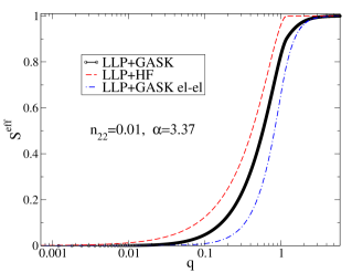
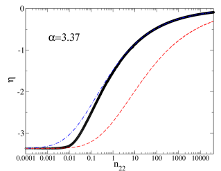
Figure 1: Upper Panel: The effective structure factor $S_{q}^{eff}$ as a function of the wave-vector $q$ (in units of $1/R_{P}$) at $n_{22}=0.01$. Lower Panel: the polaronic band shift $\eta$ (in units of $\hbar\omega_{LO}$) as a function of $n_{22}$. In both panels, electron-phonon coupling constant $\alpha=3.37$ and different approaches: $LLP+GASK$ (black solid line) stands for many-body LLP approach with Gaskell treatment of polaron-polaron interactions, $LLP+GASK$ $el-el$ (blue dash-dot line) for the same neglecting polaronic correlations, $LLP+HF$ (red dash line) for many-body LLP approach with Hartree-Fock treatment of polaron-polaron interactions.

In this subsection, we will analyze the behavior of many static quantities calculated by means of the variational approach.

We start from the effective structure factor $S_{q}^{eff}$, which represents one of the relevant quantities for the variational approach proposed in this paper. In the upper panel of Fig. 1, we plot $S_{q}^{eff}$ as a function of the wave-vector $q$ comparing different approaches for the treatment of polaron-polaron interactions. In the case of Hartree-Fock approach ($LLP+HF$ curve in the upper panel of Fig. 1), the structure factor increases quite fast for small $q$, and it presents a discontinuity at $q=2k_{F}$. On the other hand, the structure factor obtained within the Gaskell approach ($LLP+GASK$ curve in the upper panel of Fig. 1) increases more slowly for small $q$ indicating that charge correlations are accurately treated for small values of $q$. Actually, in the limit $q\ll k_{F}$, the structure factor recovers the Bijl-Feynman formula [37]

$$S^{eff}_{q}\simeq\frac{\hbar q^{2}}{2m\Omega_{PP}(q)}=\frac{\hbar}{nV_{q}^{eff}}\frac{\omega_{PP}^{2}}{2\Omega_{PP}},$$ (27)

where $\Omega_{PP}(q)$ is the frequency of the polaronic plasmon [1, 41] given by

$$\Omega_{PP}(q)\simeq\omega_{PP}\left(1+\frac{2}{9}\frac{v_{F}^{2}q^{2}}{\omega_{PP}^{2}}\right),$$ (28)

with $v_{F}=\hbar k_{F}/m$ the Fermi velocity. As discussed below, $V_{q}^{eff}$ is always proportional to $1/q^{2}$ for small $q$, therefore, in the limit $q\rightarrow 0$, the polaronic plasmon tends to the constant value $\omega_{PP}$ given by

$$\omega_{PP}=\lim_{q\rightarrow 0}\sqrt{\frac{nq^{2}}{m}V_{q}^{eff}}.$$ (29)

Indeed, in the limit of small $q$, the effective structure factor remains quadratic as a function of $q$ confirming that the normal state of many interacting large polarons is a charged Fermi liquid [37]. In the absence of polaronic effects (distribution phonon function $f_{q}=0$), $\omega_{PP}$ concides with the plasmon frequency $\omega_{P}^{\infty}$ (the square of the electron charge is screened by $\epsilon_{\infty}$), whose order of magnitude is given by

$$\frac{\omega_{P}^{\infty}}{\omega_{LO}}\simeq 11.6\left(n_{22}\right)^{\frac{1}{2}}.$$ (30)

Therefore, even for the low particle density $n=10^{20}$ $cm^{-3}$, $\omega_{P}^{\infty}$ is larger than $\omega_{LO}$. Actually, as discussed in the next section, the main contributions to the spectral properties will come from the fermion scattering with optical phonons. Finally, as reported in Eq. (28), for $f_{q}=0$, the plasmon dispersion, quadratic as a function of the wave-vector $q$, is almost coincident with that obtained within RPA approach [37, 3].

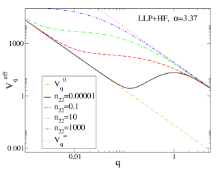
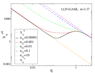
Figure 2: The effective polaron-polaron potential $V_{q}^{eff}$ (in units of $\hbar\omega_{LO}R_{P}^{3}$) as a function of the wave-vector $q$ (in units of $1/R_{P}$) for different particle densities at $\alpha=3.37$. $V_{q}^{0}$ is the bare Coulomb potential screened by the static dielectric constant $\epsilon_{0}$, while $V_{q}^{\infty}$ is the bare Coulomb potential screened by the high frequency dielectric constant $\epsilon_{\infty}$. Upper Panel: $LLP+HF$ stands for many-body LLP approach with Hartree-Fock treatment of polaron-polaron interactions. Lower Panel: $LLP+GASK$ stands for many-body LLP approach with Gaskell-RPA treatment of polaron-polaron interactions.

In order to emphasize the effects of the electron-phonon coupling on the stucture factor, in the upper panel of Fig. 1, we report $S_{q}^{eff}$ when only electron-electron interactions are taken into account within the Gaskell approach neglecting polaronic formation ($LLP+GASK$ $el-el$ in figure corresponding to the distribution phonon function $f_{q}=0$ in Eq. (25)). We remark that the self-consistent solution of the structure factor is necessary in the presence of polaronic effects for low densities. Indeed, for $n_{22}=0.01$ (shown in the upper panel of Fig. 1), the structure factor including polaronic correlations shows a behavior intermediate between the Hartree-Fock case and that obtained at $f_{q}=0$.

For many interacting polarons, the phonon function distribution $f_{q}$ given in Eq. (22) shows a behavior strongly dependent on the properties of $S^{eff}_{q}$. Within the Gaskell approach, for small values of $q$, using Eq. (22) and Eq. (27), one gets

$$f_{q}\simeq\frac{M_{q}}{\hbar\omega_{LO}+\hbar\omega_{PP}}.$$ (31)

Then, for low particle densities such that $\omega_{PP}\ll\omega_{LO}$, in the limit of small $q$, $f_{q}\simeq M_{q}/\hbar\omega_{LO}$, the characteristic distribution function of the single polaron. Otherwise, for high particle densities such that $\omega_{PP}\gg\omega_{LO}$, in the limit of small $q$, $f_{q}\simeq M_{q}/\hbar\omega_{PP}$. Therefore, polaronic effects, quantified by $f_{q}$, progressively decrease with increasing particle density. Finally, for large $q$, $f_{q}$ goes as $1/q^{3}$.

The distribution function $f_{q}$ determines the polaron shift $\eta$ defined in Eq. (15). In the lower panel of Fig. 1, we plot $\eta$ as a function of the particle density by using different treatments of the polaron-polaron interactions. In particular, in the limit of small densities, as expected, $\eta=-\alpha\hbar\omega_{LO}$ [3]. With increasing the density, $\eta$ becomes less negative, and, in the limit of high densities, it goes to zero. As shown in the lower panel of Fig. 1, the Hartree-Fock approach completely fails to describe the behavior of $\eta$ providing a systematic overestimation of the modulus of $\eta$. Actually, polaron-polaron correlations has to be necessarily included in order to correctly describe the renormalization of the polaronic band, which, as discussed in Appendix B, will provide the correction to the chemical potential $\mu$ due to many-body interactions. Finally, we point out that polaronic effects are relevant for densities up to $n_{22}=1$, which, as discussed in the following sections, can be considered as the cut-off density for the manifestation of electron-phonon effects.

Another interesting outcome of our approach is the behavior of the polaron-polaron potential $V_{q}^{eff}$, defined in Eq. (16), comparing Hartree-Fock approximation and Gaskell approach. This comparison confirms that the Hartree-Fock approach does not correctly describe the behavior of static quantities with increasing particle density.

In the upper panel of Fig. 2, we plot $V_{q}^{eff}$ when the Hartree-Fock approximation is used to determine the phonon distribution function $f_{q}$. Actually, for small values of $q$, in the limit of low density, $V_{q}^{eff}$ goes toward $V_{q}^{0}=V_{q}/\epsilon_{0}$, that is the Coulomb potential screened by the static dieletric function $\epsilon_{0}$ [36]. In the limit of large values of $q$, $V_{q}^{eff}$ tends to $V_{q}^{\infty}$, the bare Coulomb potential. With increasing the density, one expects a crossover towards a regime where $V_{q}^{eff}$ tends to be more similar to $V_{q}^{\infty}$ for smaller values of $q$. However, even for the high density $n_{22}=1000$, this crossover is not complete within the Hartree-Fock approach. Therefore, in the next section, we will analyze dynamic quantities including always correlations beyond Hartree-Fock approximation.

In the lower panel of Fig. 2, we report $V_{q}^{eff}$ when the Gaskell approach is used to determine the phonon distribution function $f_{q}$. In particular, in the limit of large $q$, by using Eq. (8), at the leading order, $V_{q}^{eff}\simeq V_{q}^{\infty}$. Instead, for small values of the wave-vector $q$, by using Eq. (27), one gets

$$V_{q}^{eff}\simeq V_{q}^{\infty}+\left(V_{q}^{0}-V_{q}^{\infty}\right)\left[1-\frac{\omega_{PP}^{2}}{(\omega_{LO}+\omega_{PP})^{2}}\right].$$ (32)

For low particle densities such that $\omega_{PP}\ll\omega_{LO}$, in the limit of small $q$, $V_{q}^{eff}\simeq V_{q}^{0}$. Otherwise, for large particle densities such that $\omega_{PP}\gg\omega_{LO}$, in the limit of small $q$, $V_{q}^{eff}\simeq V_{q}^{\infty}$. Actually, neglecting polaronic effects ($f_{q}=0$), from Eq. (30), one can determine the crossover density $n_{22}^{c}$ defined such that $\omega_{P}^{\infty}\simeq\omega_{LO}$: $n_{22}^{c}\simeq 0.01$. In fact, as shown in the lower panel of Fig. 2, at $n_{22}=0.01$, $V_{q}^{eff}$ seems to be intermediate between $V_{q}^{\infty}$ and $V_{q}^{0}$ for low values of $q$.

In contrast with Hartree-Fock approximation, we notice that, within the Gaskell approach, the crossover of $V_{q}^{eff}$ from $V_{q}^{0}$ to $V_{q}^{\infty}$ is very rapid with increasing the particle density. Indeed, as shown in the lower panel of Fig. 2, already at $n_{22}=0.1$, the crossover is almost complete. Really, at $n_{22}=10$, $V_{q}^{eff}$ is practically identical to $V_{q}^{\infty}$. Apparently, as discussed in the next section, in order to calculate the spectral properties, one needs to include a proper screening of the polaron-polaron interactions through the effects of excited states.

III Spectral properties

In the previous section, we have characterized relevant terms of the transformed Hamiltonian $\tilde{H}$ in Eq. (12). In this section, the approach used to calculate the spectral properties will be based upon an accurate many-body perturbation theory of the interaction terms in the transformed Hamiltonian $\tilde{H}$. The small effects due to the anharmonic term $H_{pol-2ph}$ in Eq. (12) are neglected focusing on the effects of the terms $H_{pol-pol}$ in Eq. (13) and $H_{pol-ph}$ in Eq. (17). The electron spectral properties of the system are calculated at zero temperature for a finite density $n$ of charge carriers in the regime from weak to intermediate electron-phonon coupling constant. In the absence of polaronic effects (distribution phonon function $f_{q}=0$), this theory recovers the approach valid in the perturbative regime of electron-electron and electron-phonon coupling [3].

After performing the canonical transformation given in Eq. (11), within the perturbative approach, the two-point electron correlation function can be disentangled into polaronic and phononic contributions [1, 44, 45, 46, 47] yielding the following electronic Green’s function ${\mathcal{G}}\left({\bf k},i\hbar k_{n}\right)$ in fermionic Matsubara frequencies $k_{n}$

$${\mathcal{G}}\left({\bf k},i\hbar k_{n}\right)=e^{-S}{\mathcal{G}}_{pol}\left({\bf k},i\hbar k_{n}\right)+$$

$$\frac{e^{-S}}{V}\sum_{\bf{k}_{1}}\sum_{l=1}^{\infty}\frac{1}{l!}F_{l}({\bf k}-{\bf k}_{1})[{\mathcal{G}}_{pol}\left(k_{1},i\hbar k_{n}+l\hbar\omega_{LO}\right)n_{F}(\xi_{k_{1}})$$

$$+{\mathcal{G}}_{pol}\left(k_{1},i\hbar k_{n}-l\hbar\omega_{LO}\right)\{1-n_{F}(\xi_{k_{1}})\}],$$ (33)

where $S=K({\bf r}=0)$, with the function $K({\bf r})$ given in terms of the distribution function $f_{q}$ as

$$K({\bf r})=\frac{1}{V}\sum_{{\bf q}}f^{2}_{q}\cos{\left({\bf q}\cdot{\bf r}\right)},$$ (34)

the function $F_{l}({\bf p})$ is defined as

$$F_{l}({\bf p})=\int d{\bf r}e^{-i{\bf p}\cdot{\bf r}}\left[K({\bf r})\right]^{l},$$ (35)

$\xi_{k}=\epsilon_{k}-\mu$, with $\epsilon_{k}$ polaronic band given in Eq. (14), and $n_{F}(E)=\theta(\mu-E)$ is the Fermi distribution function at zero temperature, with $\mu$ chemical potential. In Eq. (33), ${\mathcal{G}}_{pol}\left({\bf k},i\hbar k_{n}\right)$ is the polaron Green’s function, defined starting from the transformed Hamiltonian $\tilde{H}$ of Eq. (12).

We point out that two physically distinct terms appear in Eq. (33): the coherent and the incoherent one [42, 43]. The first term derives from the coherent motion of electrons and their surrounding phonon cloud. Without many-body corrections in the Hamiltonian $\tilde{H}$ of Eq. (12), the first term of the spectral function derived from Eq. (33) represents the purely polaronic band contribution and shows a delta behavior. This coherent term is controlled by the exponential $e^{-S}$, which will represent the most important contribution to the spectral weight of the Green’s function. On the other hand, the second term in Eq. (33) describes the possibility of changing the number of phonons in the phonon cloud during the electron motion. This is confirmed by the presence of phonon replicas and the sum over all momenta. This second term provides the incoherent contribution and spread over a wide energy range.

The polaronic Green’s function ${\mathcal{G}}_{pol}\left({\bf k},i\hbar k_{n}\right)$ in Eq. (33) is related to the polaronic self-energy $\Sigma_{pol}\left({\bf k},i\hbar k_{n}\right)$ by means of the Dyson equation [3]:

$${\mathcal{G}}_{pol}\left({\bf k},ik_{n}\right)=\frac{{\mathcal{G}}^{(0)}_{pol}\left({\bf k},ik_{n}\right)}{1-{\mathcal{G}}^{(0)}_{pol}\left({\bf k},ik_{n}\right)\Sigma_{pol}\left({\bf k},i\hbar k_{n}\right)},$$ (36)

where ${\mathcal{G}}^{(0)}_{pol}\left({\bf k},ik_{n}\right)$ is the free polaron Green’s function. Indeed, the introduction of the polaronic self-energy allows to include directly additional dampings and energy renomalizations for the large polarons improving the approximations for the calculation of the spectral properties [1, 44, 45, 46, 47]. We have checked that the self-energy does not change the spectral properties in a considerable manner, although it allows to eliminate the delta behavior in the expression of the coherent term of the spectral function.

In order to determine the polaronic self-energy, we have to evaluate the total dynamic polaron potential ${\cal W}^{(tot)}_{{\bf k},{\bf p},{\bf q}}(i\hbar q_{n})$ in bosonic Matsubara frequencies $q_{n}$, which, due to the complex polaron-phonon vertex of $\tilde{H}$, depends not only on the phononic momentum $\hbar{\bf q}$, but also on both the incoming polaronic momenta $\hbar{\bf k}$ and $\hbar{\bf p}$. Actually, with increasing the particle density, it is necessary to properly screen the polaron-polaron interaction and the polaron-phonon couplings in the limit of small $q$. In this paper, the screening is introduced by the dielectric function $\epsilon_{q}(i\hbar q_{n})$ in bosonic Matsubara frequencies $q_{n}$, which, in general, includes contributions from electron-electron and electron-phonon interactions [3]. Therefore, the total potential ${\cal W}^{tot}_{{\bf k},{\bf p},{\bf q}}(i\hbar q_{n})$ is derived as

$${\cal W}^{tot}_{{\bf k},{\bf p},{\bf q}}(i\hbar q_{n})=\frac{{\cal W}^{(0)}_{{\bf k},{\bf p},{\bf q}}(i\hbar q_{n})}{\epsilon_{q}(i\hbar q_{n})},$$ (37)

where the bare potential ${\cal W}^{(0)}_{{\bf k},{\bf p},{\bf q}}(i\hbar q_{n})$ is

$${\cal W}^{(0)}_{{\bf k},{\bf p},{\bf q}}(i\hbar q_{n})=V^{eff}_{q}+{\cal W}^{(ph)}_{{\bf k},{\bf p},{\bf q}}(i\hbar q_{n}),$$ (38)

with $V^{eff}_{q}$ the static polaron potential defined in Eq. (16), and ${\cal W}^{(ph)}_{{\bf k},{\bf p},{\bf q}}(i\hbar q_{n})$ the phonon-mediated dynamic potential.

The phonon-mediated dynamic potential ${\cal W}^{(ph)}_{{\bf k},{\bf p},{\bf q}}(i\hbar q_{n})$ in Eq. (38) comes from integrating out the phonon degrees of freedom interacting with polarons through the term $H_{pol-ph}$ of $\tilde{H}$ in Eq. (12), hence, in bosonic Matsubara frequencies $q_{n}$,

$${\cal W}^{(ph)}_{{\bf k},{\bf p},{\bf q}}(i\hbar q_{n})=\left[\left(M_{q}^{eff}\right)^{2}+U^{(0)}_{{\bf k},{\bf p},{\bf q}}\right]{\cal D}^{(0)}(i\hbar q_{n}),$$ (39)

where $M_{q}^{eff}$ is the effective polaron-phonon matrix element defined in Eq. (18), $U^{(0)}_{{\bf k},{\bf p},{\bf q}}$ is the term derived from $H^{(2)}_{pol-ph}$ given in Eq. (19)

$$U^{(0)}_{{\bf k},{\bf p},{\bf q}} = -N_{{\bf k},{\bf k}+{\bf q}}N_{{\bf p},{\bf p}-{\bf q}}$$

$$= f_{q}^{2}\left(\frac{\hbar^{2}}{2m}\right)^{2}(2{\bf k}\cdot{\bf q}+q^{2})(2{\bf p}\cdot{\bf q}-q^{2}),$$

where ${\bf k}$ and ${\bf p}$ are the incoming wave-vectors, ${\bf k}+{\bf q}$ and ${\bf p}-{\bf q}$ the outgoing wave-vectors, $N_{{\bf k},{\bf k}+{\bf q}}$ is the polaron-phonon matrix element in Eq. (20), and ${\cal D}^{(0)}(i\hbar q_{n})$ is the free phonon Green function in Matsubara frequencies $q_{n}$

$${\cal D}^{(0)}(i\hbar q_{n})=\frac{2\hbar\omega_{LO}}{(i\hbar q_{n})^{2}-(\hbar\omega_{LO})^{2}}.$$ (41)

For the calculation of the self-energy, we have to consider

$$U^{(0)}_{{\bf k},{\bf k}+{\bf q},{\bf q}}=f_{q}^{2}\left(\frac{\hbar^{2}}{2m}\right)^{2}\left(2{\bf k}\cdot{\bf q}+q^{2}\right)^{2},$$ (42)

which is a positive quantity like $\left(M_{q}^{eff}\right)^{2}$, but it depends on the angle between ${\bf k}$ and ${\bf q}$. We remark that $U^{(0)}_{{\bf k}_{1},{\bf k}_{1}+{\bf q},{\bf q}},$, with ${\bf k}_{1}=k_{F}{\hat{q}}$, is equal to the coupling $T_{2,q}$, which, in addition to $T_{1,q}=\left(M_{q}^{eff}\right)^{2}$, is analyzed in Appendix A. As discussed in this Appendix, the two polaron-phonon coupling terms $T_{1,q}$ and $T_{2,q}$ provide comparable contributions to the spectral properties in the intermediate electron-phonon coupling regime for low particle densities.

After having evaluated the total polaron potential ${\cal W}^{(tot)}_{{\bf k},{\bf p},{\bf q}}(i\hbar q_{n})$, the polaronic self-energy to the lowest order can be obtained as

$$\Sigma_{pol} \left({\bf k},i\hbar k_{n}\right)=$$

$$-\frac{1}{\beta V}\sum_{{\bf q},q_{n}}{\cal W}^{(tot)}_{{\bf k},{\bf k}+{\bf q},{\bf q}}(i\hbar q_{n}){\mathcal{G}}^{(0)}_{pol}\left({\bf k}+{\bf q},i\hbar k_{n}+i\hbar q_{n}\right),$$

where $\beta=1/k_{B}T$, with $k_{B}$ Boltzmann constant, $T$ temperature. Making the analytic continuation $i\hbar k_{n}\rightarrow E+i\delta$, with $\delta$ infinitesimal quantity, and the limit to zero temperature, Eqs. (33) and (36) allow to evaluate the retarted electronic Green’s function $G^{ret}({\bf k},E)$ and the electronic spectral function $A({\bf k},E)=-2\Im G^{ret}({\bf k},E)$, which will be thoroughly discussed in the next subsections. We have checked that the sum rule $\int_{-\infty}^{+\infty}\frac{dE}{2\pi}A({\bf k},E)=1$ is satisfied with a tolerance of a few per cent for all the electron-phonon coupling regimes and particle densities analyzed in this paper.

III.1 Single polaron - low density regime in STO-based systems

In the limit of very low particle density, analytic calculations can be made to determine many contributions to the spectral function not only within the electron-phonon perturbative regime [27, 48], but also within the LLP approach. In particular, we focus on the spectral weight at $k=0$, indicated with $Z_{0}$, which represents a relevant measure of the polaronic character in the case of a single fermion [3].

The scheme perturbative in the electron-phonon coupling provides the following estimate for $Z_{0}$:

$$Z_{0}^{PERT}=\frac{1}{1+\frac{\alpha}{2}},$$ (44)

such that, for very low $\alpha$, $Z_{0}^{PERT}\simeq 1-\alpha/2$, which is commonly used in the literature [3]. In any case, as shown in the upper panel of Fig. 3, the spectral weight decreases with increasing the coupling constant $\alpha$. In the same panel, we report the spectral weight calculated within the LLP scheme:

$$Z_{0}^{LLP}=\exp{\left(-\frac{\alpha}{2}\right)},$$ (45)

We point out that $Z_{0}^{LLP}$ represents a very relevant contribution to the exact spectral weight. Indeed, as shown in the upper panel of Fig. 3, $Z_{0}^{LLP}$ is slightly larger than the numerically exact results from DQMC technique. For $\alpha>4$, the spectral weight is smaller than $0.1$, therefore, the spectral function derived from Eq. (33) is dominated by the incoherent term. This is the reason why, in the lower panel of Fig. 3, we focus on the spectral functions for $\alpha<4$. In particular, for $\alpha=3.37$, which is the value estimated to be relevant for STO-based systems, $Z_{0}$ is very close to $0.2$, hence, the quasi-particle, the large polaron, is still well defined. As shown in the next subsection, this value of $Z_{0}$ for $\alpha=3.37$ is in very good agreement with its estimate from experimental data in the limit of small particle densities [14].

Figure 3: Upper Panel: Single fermion spectral weight at wave-vector $k=0$ as a function of the electron-phonon coupling constant $\alpha$ for different approaches: $PERT$ stands for perturbative approach, $LLP$ for Lee-Low-Pines method, $LLP+PERT$ for perturbative corrections upon LLP method, $DQMC$ for Diagrammatic Quantum Monte-Carlo data from Ref. [25]. Lower Panel: Single fermion spectral function (in units of $1/\hbar\omega_{LO})$ at wave-vector $k=0$ as a function of the energy (related to the ground state energy $E_{0}$, both in units of $\hbar\omega_{LO}$) at $k=0$ for different values of the electron-phonon coupling constant $\alpha$ within the perturbative method upon the LLP approach (LLP+PERT). A negligible width $\Gamma$ has been added as an imaginary part to the polaronic self-energy.

In order to go beyond the LLP scheme and to determine the polaronic self-energy $\Sigma_{pol}\left({\bf k},i\hbar k_{n}\right)$, in the case of a single fermionic particle, we only need ${\cal W}^{(ph)}$ in Eq. (39), thus, making the limit of very low particle density for all the quantities, ${\cal W}^{(tot)}={\cal W}^{(ph)}$. Analytic calculations can be made to determine the retarded polaronic self-energy $\Sigma_{pol}^{ret}\left({\bf k},E\right)$. In particular, including the lowest order polaron-phonon corrections upon the LLP scheme, the spectral weight at $k=0$, $Z_{0}^{LLP+PERT}$, is

$$Z_{0}^{LLP+PERT}=Z_{0}^{LLP}\cdot Z_{0}^{PERT}=\frac{\exp{\left(-\frac{\alpha}{2}\right)}}{1+\frac{\alpha}{8}}.$$ (46)

Therefore, the polaron-phonon correction provides a denominator which is similar to that obtained for the electron-phonon perturbation theory given in Eq. (44). As expected, the fraction in the denominator is smaller than that present in Eq. (44) since the polaron-phonon interaction terms are reduced in comparison with the bare electron-phonon vertex. As shown in the upper panel of Fig. 3, $Z_{0}^{LLP+PERT}$ is in excellent agreement with numerical DQMC data suggesting that weak polaron-phonon corrections are effective to improve the accuracy of the spectral properties.

Next, we analyze the polaron effective mass at $k=0$, denoted with $m_{0}^{*}$, which quantifies the mass increase due to the phonon cloud accompanying the electron [3]. The approach perturbative in the electron-phonon coupling provides the following estimate for $m_{0}^{*}$:

$$\frac{m}{m_{0}^{*}}=\left(1+\frac{\alpha}{3}\right)\cdot Z_{0}^{PERT}=\frac{1+\frac{\alpha}{3}}{1+\frac{\alpha}{2}}>Z_{0}^{PERT},$$ (47)

such that, for very low $\alpha$, $\frac{m}{m_{0}^{*}}\simeq 1-\frac{\alpha}{6}$, which is typically used in the literature [3].

In Appendix B we provide some details concerning the dispersion of the polaron as a function of the wave-vector. In particular, as discussed in this Appendix, the evaluation of the polaronic self-energy in the case of a single fermion allows to estimate also the effective mass. It is found that, for $\alpha<4$, the effective mass at $k=0$ is well approximated by the following expression which extends the perturbative estimate to the intermediate coupling regime: $\frac{m}{m_{0}^{*}}\simeq 1-\frac{\alpha}{6}$. Indeed, the corrections to the mass for the Fröhlich single polaron are power laws in the constant coupling $\alpha$ within the intermediate electron-phonon coupling regime, therefore they are weaker than those, exponential in $\alpha$, characteristic of the spectral weight [25]. Moreover, for $\alpha=3.37$, value relevant for STO-based systems, $\frac{{m_{0}^{*}}}{m}\simeq 2.28$. We remark that this value is in very good agreement with the experimental estimate $\frac{{m_{0}^{*}}}{m}\simeq 2.33$ obtained in the limit of low particle densities [14].

Finally, we focus on the spectral function at $k=0$ derived from Eq. (33) in the limit of low particle density. In the lower panel of Fig. 3, we plot the spectral function at $k=0$ as a function of the energy for different values of the electron-phonon coupling constant $\alpha$. We notice that the all the curves show the peak-dip-hump structure characteristic of the experimental spectral function [14, 16, 12]. The peak corresponds to the coherent term, while the hump to the incoherent contribution. Therefore, the increase of the coupling constant $\alpha$ induces a transfer of spectral weight towards higher energies enhancing the number of phonon satellites. In fact, for $\alpha=0.5$, one-phonon satellite is evident in the spectra, while, for $\alpha=3.37$, coupling relevant for STO-based systems, at least three phonon satellites characterize the incoherent term. We remark that these features of the spectrum for $\alpha=3.37$ are in very good agreement with the electron spectral function extracted from experiments in the limit of low particle density [14].

Summarizing, not only spectral weight and effective mass, but also the spectral function at $k=0$ in the limit of small density are accurately described by the approach used in this paper confirming that the estimated value $\alpha=3.37$ is perfectly consistent with experimental results in STO-based systems. In the next subsections, we analyze the effects of a finite particle density for which polaron-polaron interactions become relevant together with polaron-phonon couplings.

III.2 RPA-Gaskell approach - low to high density regime in STO-based systems

We recall that the calculation of the electronic Green’s function ${\mathcal{G}}\left({\bf k},ik_{n}\right)$ in Eq. (33) requires the evaluation of the polaronic Green’s function ${\mathcal{G}}_{pol}\left({\bf k},ik_{n}\right)$ in Eq. (36) and its phonon replicas. In turn, the polaronic Green’s function is calculated through the polaronic self-energy $\Sigma_{pol}\left({\bf k},i\hbar k_{n}\right)$, which requires the total dynamic polaron potential ${\cal W}^{tot}_{{\bf k},{\bf k}+{\bf q},{\bf q}}(i\hbar q_{n})$ in Eq. (37) obtained by screening the bare polaron potential ${\cal W}^{(0)}_{{\bf k},{\bf k}+{\bf q},{\bf q}}(i\hbar q_{n})$ given in Eq. (38) through the dielectric function $\epsilon_{q}(i\hbar q_{n})$.

At the level of the Hartree-Fock approximation, in Eq. (37), the dielectric function is approximated to unity, therefore the total dynamical potential reduces to the bare one ${\cal W}^{(0)}$: ${\cal W}^{(tot)}={\cal W}^{(0)}$. Therefore, screening effects due to the presence of fermionic charge carriers are not included in the dynamical potential. As expected, at the Hartree-Fock level, the effects of a finite density $n$ of charge carriers are not correctly taken into account. In this paper, the calculation of the dielectric function is made extending the Gaskell approach beyond the ground state which has been analyzed in the previous section. Since the results are similar to the RPA approach, we call this method RPA-Gaskell.

We have checked that a very accurate starting point to calculate the dielectric function is the self-consistent structure factor $S_{q}^{eff}$ which, for small $q$, satisfies the Bijl-Feynman relation in Eq. (27) related to the polaron plasmon $\Omega_{PP}(q)$ in Eq. (28). Indeed, we recall that the static structure factor can be obtained for $q\neq 0$ as

$$S_{q}^{eff}=\int_{0}^{\infty}\frac{d\hbar\omega}{\pi}S_{q}^{eff}(\hbar\omega),$$ (48)

where $S_{q}^{eff}(\hbar\omega)$ is the dynamic structure factor, which is the spectral function of the retarded inverse dielectric function $\epsilon_{q}^{ret}(\hbar\omega)$ [3]:

$$S_{q}^{eff}(\hbar\omega)=-\frac{1}{nV_{q}^{eff}}\Im\left[\frac{1}{\epsilon_{q}^{ret}(\hbar\omega)}\right],$$ (49)

with $\epsilon_{q}^{ret}(\hbar\omega)$ derived from $\epsilon_{q}(i\hbar q_{n})$ through the analytic continuation $q_{n}\rightarrow\omega+i\delta$ ($\delta$ is an infinitesimal quantity). In order to satisfy the Bijl-Feynman relation of Eq. (27) for small $q$, the inverse dielectric function in Matsubara frequencies must have the following form:

$$\frac{1}{\epsilon_{q}(i\hbar q_{n})} =1+\frac{\hbar\omega_{PP}^{2}}{2\Omega_{PP}(q)}\times$$

$$\left[\frac{1}{i\hbar q_{n}-\hbar\Omega_{PP}(q)}-\frac{1}{i\hbar q_{n}+\hbar\Omega_{PP}(q)}\right],$$

with $\omega_{PP}$ the polaron plasmon at zero wave-vector given in Eq. (29). Therefore, as expected for small values of $q$, the dielectric function is dominated by plasmon poles [49], which are related to the polaron plasmon with frequency $\Omega_{PP}(q)$. This is the dielectric function that can be used in Eq. (37) to accurately screen polaron-polaron and polaron-phonon interactions.

Since dynamic effects due to plasmons have not been identified in the electronic spectral properties of STO-based systems, we focus on the static dielectric function $\epsilon_{q}$ which, as expected, goes as $1/q^{2}$ for small values of $q$:

$$\epsilon_{q}=1+\frac{\omega_{PP}^{2}}{\Omega_{PP}^{2}(q)-\omega_{PP}^{2}}=1+\frac{q_{GFT}^{2}}{q^{2}},$$ (51)

where $q_{GTF}$ is a generalized Thomas-Fermi wave-vector, defined as

$$q_{GTF}=\frac{3}{2}\frac{\omega_{PP}}{v_{F}},$$ (52)

with $v_{F}$ Fermi velocity. In fact, in the absence of polaronic effects ($f_{q}=0$), $\epsilon_{q}$ is practically coincident with the Thomas-Fermi dielectric function, which provides an accurate screening of the long-range electron-electron potential for small values of $q$ and is frequently used also for screening the potential due to the electron-phonon coupling [3]. As a result, for the evaluation of the potential in Eq. (37) and the related polaronic self-energy, we will use the static dielectric function given in Eq. (51).

First, we focus on $Z_{F}$, the spectral weight at the Fermi wave-vector $k_{F}$, which is derived from the Green’s function in Eq. (33). Really, this renormalization factor plays the role of the residue at the pole in a Fermi-liquid description [50]. Thus, we can evaluate the renormalized electron distribution function $n^{ren}_{{\bf k}}=\int_{-\infty}^{+\infty}\frac{dE}{2\pi}A({\bf k},E)n_{F}(E)$. At zero temperature, we recall that $n^{ren}(\mu-\delta)-n^{ren}(\mu+\delta)=Z_{F}$ (with $\delta$ infinitesimal energy), so that the factor $Z_{F}$ determines the jump in the Fermi distribution function [42]. Actually, the polaronic self-energy introduces tiny differences between $Z_{F}$ and the renormalization term $e^{-S}$ in Eq. (33) only in the low density regime, since, with increasing the particle density, screening rapidly reduces the effects due to polaron-polaron and polaron-phonon interactions.

In the upper panel of Fig. 4, we plot $Z_{F}$ as a function of the two-dimensional particle density $n_{2D}$ for different values of the electron-phonon constant $\alpha$. We recall that the two-dimensional $n_{2D}$ is obtained from the three-dimensional density $n$ through the effective length $d=6$ nm. For any value of the coupling constant $\alpha$, $Z_{F}$ gets enhanced with increasing the particle density. We stress that this increase starts from around $n_{2D}=6\cdot 10^{12}$ $cm^{-2}$, and it is very rapid from $n_{2D}=6\cdot 10^{13}$ $cm^{-2}$. Indeed, at $n_{2D}=6\cdot 10^{14}$ $cm^{-2}$, the spectral weights for different values of $\alpha$ converge towards similar values. Finally, at $n_{2D}=6\cdot 10^{16}$ $cm^{-2}$, $Z_{F}$ is close to unity for any value $\alpha$ indicating that the screening of many-body interactions is almost complete. For these values of the density, polaronic effects are very weak, therefore the system presents a conventional metallic state.

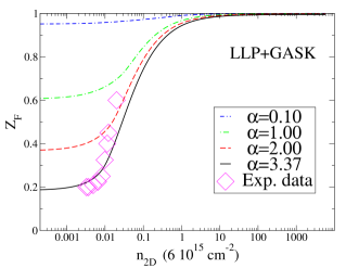
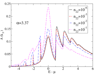
Figure 4: Upper Panel: Spectral weight at Fermi wave-vector $k_{F}$, $Z_{F}$, as a function of the particle density $n_{22}$ for different values of the electron-phonon constant $\alpha$ within the many-body LLP approach with Gaskell-RPA treatment of polaron-polaron interactions (LLP+GASK). Experimental data are taken from Ref. [14]. Lower Panel: Spectral function (in units of $1/\hbar\omega_{LO})$ at Fermi wave-vector $k_{F}$ as a function of the energy (related to the chemical potential $\mu$, both in units of $\hbar\omega_{LO}$) for different values of particle density at $\alpha=3.37$ within the many-body perturbative method upon the LLP approach. A width $\Gamma=0.5\hbar\omega_{0}$ has been added as an imaginary part to the polaronic self-energy.

It is important to note that these results are compatible with photoemission experiments at the $(001)$ STO surface [14]. Indeed, as shown in the upper panel of Fig. 4, not only the low density value of $Z_{F}$ but also its calculated behavior as a function of the particle density agree with experimental data. In particular, with increasing the particle density, the experimental enhancement of $Z_{F}$ looks a little bit more marked than that predicted by theory. We notice that the two-dimensional behavior is predicted by theory taking into account the effective length $d$ of the electron gas. One expects that screening effects beyond Hartree-Fock approximation would be more pronounced in an actual two-dimensional calculation providing a more rapid increase of the spectral weight $Z_{F}$.

The next step is to analyze the spectral function derived from the Green’s function in Eq. (33). In the lower panel of Fig. 4, fixing $\alpha=3.37$, we report the spectral function at the Fermi wave-vector $k_{F}$ as a function of the energy for different densities considering both the hole ($E<\mu$) and the particle sector ($E>\mu$). The peak-dip-hump line shape is recovered not only for low densities, but also for high densities. With increasing carrier concentration, a transfer of spectral weight occurs towards the coherent peak by reducing the hump consisting of phonon satellites due to the incoherent large polaron dynamics. Moreover, this transfer towards the coherent peak is accompanied by an increase of the spectral weight of the hole sector with increasing density. We remark that experiments in Ref. [14] show only the hole sector, which is very carefully described by out theory. For example, as shown in the lower panel of Fig. 4, in contrast with the behavior in the particle sector, the coherent peak is higher than the first phonon satellite in the hole sector for all the charge densities. Actually, in the lower panel of Fig. 4, we have added width $\Gamma=0.5\hbar\omega_{0}$ as an imaginary part to the polaronic self-energy in order to simulate the instrumental resolution of photoemission spectra and to make a more realistic comparison with experiments. Moreover, in agreement with experiments [14], we recognize three different density regimes: the first one corresponding to quite low densities ($n_{22}\leq 10^{-4}$), the second one to intermediate densities ($10^{-4}<n_{22}<10^{-1}$), the third one to high densities ($n_{22}\geq 10^{-1}$). In the final part of the paper, we analyze these three regimes.

In the first regime at low densities, the spectral function is not identical to that in the limit of single polaron discussed in a previous subsection, since, as shown in the lower panel of Fig. 4 for $n_{22}=10^{-6}$, there is also the incoherent hole contribution for energies below the chemical potential. Even if the incoherent hole hump has less spectral weight than the incoherent electron hump, the number of phonon satellites in the two humps is very similar confirming that polaronic effects are active both in the hole and particle channel. In this first regime with low density, screening is not active, therefore, electrons interact with phonons through a long range Fröhlich coupling.

In the second regime of intermediate density ($10^{-4}<n_{22}<10^{-1}$), screening starts to reduce polaronic effects whose spatial range decreases with increasing density. Indeed, as shown in the lower panel of Fig. 4 for $n_{22}=10^{-3}$ and $n_{22}=10^{-2}$, the number of phonon satellites is reduced transferring spectral weight to the coherent peak. We stress that this coherent-incoherent crossover is quite rapid: for $n_{22}=10^{-3}$ (corresponding to $n_{2D}$ of the order of $10^{13}$ $cm^{-2}$), the satellite structure is not dissimilar from that of lower densities, on the other hand, for $n_{22}=10^{-2}$ (corresponding to $n_{2D}$ of the order of $10^{14}$ $cm^{-2}$), only the first phonon satellite is marked, the second one is strongly reduced, the third one has almost completely disappeared. All these features are in excellent agreement with tunneling and photoemission experiments probing the polaronic liquid in STO-based systems [14, 13].

In the third regime at high densities ($n_{22}\geq 10^{-1}$), screening becomes predominant causing the breakdown of the polaronic state. As shown in the lower panel of Fig. 4 for $n_{22}=10^{-1}$, the weight of the coherent term is prevalent. The system behaves as a metal with a short range electron-phonon coupling. Indeed, in this regime, the mass ratio at the Fermi wave-vector $k_{F}$, $\frac{m}{m_{F}^{*}}$, becomes very similar to the spectral weight $Z_{F}$, confirming the short range character of many-body interactions.

Summarizing, the variation of carrier concentration controls the screening of many-body interactions affecting the spectral properties of large polaron systems. From the comparison between the lower panels of Figs. 3 and 4, it emerges that the role of density can be roughly understood as an effect leading to the reduction of the electron-phonon coupling constant. An estimate of this reduction as a function of the particle density is not easy since it involves both polaron features and many-body screening, which, in our work, are intimately linked.

IV Conclusions and discussions

In this paper, we have discussed ground state and spectral properties of the Fröhlich model as a function of the particle density focusing on the intermediate electron-phonon coupling regime at zero temperature. We have introduced a new variational approach exploring a huge range of particle densities. The formation of the large polaron and the role of screening turn out to play a crucial role in understanding the spectral properties of STO-based systems with varying the carrier concentration. In the case of a single polaron, the peak-dip-hump line shape is in good agreement with the spectral function obtained by numerical approaches and with experimental spectra of STO-based systems in the low density limit. In addition to the low density regime, we have identified other two relevant density ranges, the intermediate and high density ones. While for high densities the system shows a conventional metallic phase, for intermediate densities, a rapid crossover takes place from incoherent to coherent large polaron dynamics with increasing carrier density finding very good agreement with experimental spectra in STO-based systems.

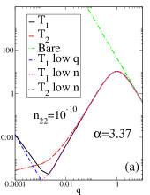
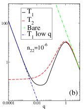
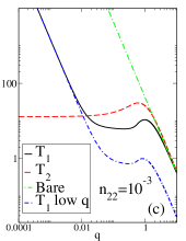
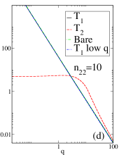
Figure 5: Polaron-phonon couplings (in units of $(\hbar\omega_{LO})^{2}R^{3}_{P}$) as a function of the wave-vector $q$ (in units of $1/R_{P}$) at electron-phonon coupling constant $\alpha=3.37$ for $n_{22}=10^{-10}$ (Panel (a)), $n_{22}=10^{-6}$ (Panel (b)), $n_{22}=10^{-3}$ (Panel (c)), $n_{22}=10$ (Panel (d)). $T_{1}$ $low$ $q$ stands for the low $q$ expansion of the coupling $T_{1}$, $T_{1}$ $low$ $n$ for the low density expansion of the coupling $T_{1}$, $T_{2}$ $low$ $n$ for the low density expansion of the coupling $T_{2}$, $Bare$ for the bare coupling given by the square of $M_{q}$ defined in Eq. (8).

In this work, we have ascribed all the electron-phonon coupling to a single longitudinal optical mode with frequency $\omega_{LO}$ which is mostly coupled to charge carriers. This mode has quite a high frequency ($\hbar\omega_{LO}\simeq 100$ meV), therefore we have largely analyzed the antiadiabatic regime relative to this mode (Fermi energy $E_{F}$ such that $E_{F}<\hbar\omega_{LO}$) Additional low frequency optical modes are present, however, they are much more weakly coupled to the electrons [12, 13]. Tiny spectral features due to these modes can be recognized in tunneling experiments [13], but are not visible in photoemission data [14]. Indeed, due to instrumental resolution of photoemission experiments, the main peak shown in the experimental data at the Fermi energy is quite large. We have estimated a width of the order of $\Gamma=0.5\hbar\omega_{0}$. Therefore, in photoemission experiments, the main peak at the Fermi energy could include not only the coherent peak but also the first satellites due to low frequency optical modes. This is the reason why, in the literature, the modeling of spectral properties has been done in the perturbative electron-phonon coupling regime considering only the most coupled high frequency mode [14]. We point out that additional phonon modes can be included into the theoretical model since this involves a simple generalization of our approach.

In this work, we have focused on the spectral properties of the normal state at zero temperature. The next step could be the analysis of superconducting states [6, 7] where the coupling to longitudinal optical phonons plays a non negligible role [51, 52]. Finally, another interesting aspect could be related to the role of electron-phonon coupling on the temperature behavior of spectral and transport properties [16, 53, 54], for example of the thermoelectric Seebeck effect [55, 56].

Appendix A Polaron-phonon couplings

In this Appendix, we discuss the polaron-phonon couplings of the transformed Hamiltonian $\tilde{H}$ in Eq. (12), which, in addition to the polaron-polaron potential $V_{q}^{eff}$, are relevant for the evaluation of the spectral properties presented in the main text.

We start considering the first coupling $T_{1,q}$, defined as

$$T_{1,q}=\left(M_{q}^{eff}\right)^{2}=M_{q}^{2}\frac{\left[\frac{\hbar^{2}q^{2}}{2mS_{q}^{eff}}\right]^{2}}{\left[\hbar\omega_{LO}+\frac{\hbar^{2}q^{2}}{2mS_{q}^{eff}}\right]^{2}},$$ (53)

where we have used the expression of $M_{q}^{eff}$ in Eq. (18). Within the Gaskell approach, for small values of the wave-vector $q$,

$$T_{1,q}\simeq M_{q}^{2}\frac{\left[\omega_{PP}\right]^{2}}{\left[\omega_{LO}+\omega_{PP}\right]^{2}}.$$ (54)

For low particle densities such that $\omega_{PP}\ll\omega_{LO}$, with $\omega_{PP}$ the polaron plasmon at zero wave-vector given in Eq. (29), in the limit of small $q$, $T_{1,q}$ is quite small. Otherwise, for large particle densities such that $\omega_{PP}\gg\omega_{LO}$, in the limit of small $q$, $T_{1,q}$ tends to the bare coupling $M_{q}^{2}$. Finally, for large values of $q$, as expected, $T_{1,q}\simeq M_{q}^{2}$.

Then, we study the second coupling $T_{2,q}$, defined as

$$T_{2,q}=\left[N_{{\bf k}_{1},{\bf k}_{1}+{\bf q}}\right]^{2}=\left(\frac{\hbar^{2}f_{q}}{2m}\right)^{2}\left[{\bf q}\cdot({\bf q}+2{\bf k}_{1}\right]^{2},$$ (55)

where we have considered the polaron-phonon matrix element in Eq. (20), with ${\bf k}_{1}=k_{F}{\hat{q}}$. Therefore, for this coupling, we consider the most relevant contribution, that is that at the Fermi wave-vector $k_{F}$ in a direction given by the versor ${\hat{q}}$ of the wave-vector ${\bf q}$. In analogy with $T_{1,q}$, $T_{2,q}$ tends towards the bare coupling $M_{q}^{2}$ for large values of $q$.

In Fig. 5 we plot the first coupling $T_{1,q}$ and the second coupling $T_{2,q}$ as a function of the modulus $q$ of the wave-vector ${\bf q}$ for different particle densities. The panel (a) corresponds to the lowest particle density $n_{22}=10^{-10}$. We notice that, for this density, $T_{1,q}$ and $T_{2,q}$ are almost identical for a large range of values of $q$. They differ only for small values of $q$, where $T_{1,q}$ increases with decreasing $q$ recovering the limit for small $q$. On the other hand, $T_{2,q}$ is always coincident with the limit for small density $n$.

The panel (b) of Fig. 5 corresponds to the low particle density $n_{22}=10^{-6}$. The couplings $T_{1,q}$ and $T_{2,q}$ coincide for large values of $q$. For intermediate values of $q$, $T_{1,q}$ is smaller than $T_{2,q}$, while, for small values of $q$, one gets the opposite. In fact, $T_{1,q}$ shows a crossover from the small $q$ limit to the bare coupling with increasing the values of $q$.

In panel (c) of Fig. 5 we plot the couplings $T_{1,q}$ and $T_{2,q}$ for the particle density $n_{22}=10^{-3}$. They differ in a large range of values of $q$. The coupling $T_{1,q}$ shows a narrower crossover from the small $q$ limit to the bare coupling. Finally, the panel (d) of Fig. 5 shows the couplings $T_{1,q}$ and $T_{2,q}$ for the particle density $n_{22}=10$. As expected, the coupling $T_{1,q}$ always coincides with the bare coupling, while the coupling $T_{2,q}$ is negligible in comparison with $T_{1,q}$ for a large range of values of $q$. As discussed in the main text, for high values of density, screening of the polaron-phonon vertex is fundamental to properly calculate the spectral properties.

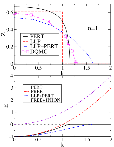
Figure 6: Upper Panel: Single fermion spectral weight as a function of the wave-vector $k$ (in units of $1/R_{P}$) for different approaches: $PERT$ stands for perturbative approach, $LLP$ for Lee-Low-Pines method, $LLP+PERT$ for perturbative corrections upon LLP method, $DQMC$ for Diagrammatic Quantum Monte-Carlo data from Ref. [25]. Lower Panel: Single fermion quasi-particle energy (in units of $\hbar\omega_{LO})$ as a function of the wave-vector $k$ (in units of $1/R_{P}$) for different approaches: $PERT$ stands for perturbative approach, $LLP+PERT$ for perturbative corrections upon LLP method, $FREE$ for the bare electronic dispersion (shifted by the ground state energy $E_{0}$), $FREE+1PHON$ for the same with a shift of $\hbar\omega_{LO}$. In both panels, electron-phonon coupling constant $\alpha=1$.

Appendix B Additional results on polaron spectral properties

In this Appendix, we provide some details concerning the dispersion of the quasi-particles as a function of the wave-vector. In particular, we discuss the evaluation of the polaronic self-energy in the case of wave-vectors different from Fermi wave-vector $k_{F}$.

In this paper, a perturbative approach is made on top of the LLP scheme, which, however, already provides quite accurate polaronic energies. Therefore, in our perturbative approach, we fix $\Re\Sigma^{ret}_{pol}(k_{F},\omega=0)=0$ [27], therefore the chemical potential is $\mu=\frac{\hbar^{2}k_{F}^{2}}{2m}+\eta$, where $\eta$ is the polaronic band shift given in Eq. (15). In the limit of single polaron, one gets the correct ground state energy $E_{0}=\eta=-\alpha\hbar\omega_{LO}$ within the intermediate electron-phonon coupling regime.

In order to investigate the behavior of spectral properties as a function of the wave-vector $k$, we analyze the single polaron case. We plot the spectral weight $Z_{k}$ as a function of the wave-vector $k$ in the upper panel of Fig. 6 comparing different approaches at $\alpha=1$. We notice the rapid decrease of the spectral weight with increasing $k$. The LLP scheme is not able to describe this behavior, while the lowest order perturbation theory on top of the LLP approach ($LLP+PERT$ in figure) is able to interpolate the DQMC numerical data. Clearly, the comparison of the approach with DQMC results could improve if one would include further corrections in the building up of the self-energy. For example, one possibility would be to make a self-consistent calculation between polaronic Green’s function and self-energy.

In addition to the spectral weight, we have derived the polaron dispersion. We plot the quasi-particle energy as a function of the wave-vector $k$ in the lower panel of Fig. 6 comparing different approaches at $\alpha=1$. There is a flattening of the polaron dispersion when the spectral weight goes to zero. This occurs when the difference between the energy at finite $k$ and that at $k=0$ is equal to the phonon energy $\hbar\omega_{LO}$ [3]. Finally, we consider the effective mass analyzing the polaron dispersion for small wave-vectors. For $\alpha=1$, the approach perturbative in the electron-phonon coupling provides the estimate $m_{0}^{*}\simeq 1.13m$, by using Eq. (47). As shown in the lower panel of Fig. 6, the dispersion calculated within the perturbation theory upon the LLP scheme has a smaller curvature. Indeed, the effective mass ratio is a little bit higher: $m_{0}^{*}\simeq 1.2m$.

References

- [1] A. S. Alexandrov and N. Mott, Polarons and Bipolarons World Scientific, Singapore (1996).
- [2] A. S. Alexandrov and J. T. Devreese, Advances in Polaron Physics Springer Series in Solid-State Sciences (159) (2010).
- [3] G. Mahan, Many-particle Physics, 2nd edn, Plenum Press, New York (1990).
- [4] A. D. Caviglia, S. Gariglio, N. Reyren, D. Jaccard, T. Schneider, M. Gabay, S. Thiel, G. Hammerl, J. Mannhart, J.-M. Triscone, Nature 456, 624 (2008).
- [5] Y.-Y. Pai, A.- Tylan-Tyler, P. Irvin, and J. Levy, Rep. Prog. Phys. 81 036503 (2018).
- [6] X. Lin, Z. Zhu, B. Fauque, and K. Behnia, Phys. Rev. X 3, 021002 (2013)
- [7] X. Lin, G. Bridoux, A. Gourgout, G. Seyfarth, S. Kramer, M. Nardone, B. Fauque, and K. Behnia, Phys. Rev. Lett. 112, 207002 (2014).
- [8] Y. Aiura, I. Hase, H. Bando, T. Yasue, T. Saitoh, D.S. Dessau, Surf. Sci. 515, 61 (2002).
- [9] M. Takizawa, K. Maekawa, H. Wadati, T. Yoshida, A. Fujimori, H. Kumigashira, and M. Oshima, Phys. Rev. B 79, 113103 (2009).
- [10] Y. J. Chang, A. Bostwick, Y. S. Kim, K. Horn, and E. Rotenberg, Phys. Rev. B 81, 235109 (2010).
- [11] W. Meevasana, X. J. Zhou, B. Moritz, C.-C. Chen, R. H. He, S.-I. Fujimori, D. H. Lu, S.-K. Mo, R. G. Moore, F. Baumberger, T. P. Devereaux, D. van der Marel, N. Nagaosa, J. Zaanen, and Z.-X. Shen, New J. Phys. 12, 023004 (2010).
- [12] V. N. Strocov, C. Cancellieri, and A. S. Mishchenko, in Spectroscopy of Complex Oxide Interfaces: Photoemission and Related Spectroscopies, eds. C. Cancellieri and V.N. Strocov, Springer Verlag (2019).
- [13] A. G. Swartz, H. Inoue, T. A. Merz, Y. Hikita, S. Raghu, T. P. Devereaux, S. Johnston, and H. Y. Hwang, PNAS 115, 1475 (2018).
- [14] Z. Wang, S. McKeown Walker, A. Tamai, Y. Wang, Z. Ristic, F. Y. Bruno, A. de la Torre, S. Ricco, N. C. Plumb, M. Shi, P. Hlawenka, J. Sanchez-Barriga, A. Varykhalov, T. K. Kim, M. Hoesch, P. D. C. King, W. Meevasana, U. Diebold, J. Mesot, B. Moritz, T. P. Devereaux, M. Radovic, F. Baumberger, Nat. Mater. 15, 835 (2016).
- [15] C. Chen, J. Avila, E. Frantzeskakis, A. Levy, and M. C. Asensio, Nat. Commun. 6, 8585 (2015).
- [16] C. Cancellieri, A. S. Mishchenko, U. Aschauer, A. Filippetti, C. Faber, O. S. Barisic, V. A. Rogalev, T. Schmitt, N. Nagaosa, and V. N. Strocov, Nat. Commun. 7, 10386 (2016).
- [17] J. L. M. van Mechelen, D. van der Marel, C. Grimaldi, A. B. Kuzmenko, N. P. Armitage, N. Reyren, H. Hagemann, and I. I. Mazin, Phys. Rev. Lett. 100, 226403 (2008).
- [18] A. Dubroka, M. Rossle, K. W. Kim, V. K. Malik, L. Schultz, S. Thiel, C. W. Schneider, J. Mannhart, G. Herranz, O. Copie, M. Bibes, A. Barthelemy, and C. Bernhard, Phys. Rev. Lett. 104, 156807 (2010).
- [19] A. Geondzhian, A. Sambri, G. M. De Luca, R. Di Capua, E. Di Gennaro, D. Betto, M. Rossi, Y. Y. Peng, R. Fumagalli, N. B. Brookes, L. Braicovich, K. Gilmore, G. Ghiringhelli, and M. Salluzzo, Phys. Rev. Lett. 125, 126401 (2020).
- [20] V. Cataudella, G. De Filippis and C.A. Perroni, in Polarons in Advanced Materials, ed. by A.S. Alexandrov (Springer, Dordrecht, 2007).
- [21] G. De Filippis., V. Cataudella, V. Marigliano Ramaglia, C. A. Perroni, and D. Bercioux, Eur. Phys. J. B. 36, 65 (2013).
- [22] G. De Filippis, V. Cataudella, A. S. Mishchenko, C. A. Perroni, and J. T. Devreese, Phys. Rev. Lett. 96, 136405 (2006).
- [23] T. D. Lee, F. E. Low, and D. Pines, Phys. Rev. 90, 292 (1953).
- [24] A. Chatterjee, and S. Mukhopadhyay, Polarons and Bipolarons: An Introduction, CRC Press (2018).
- [25] A. S. Mishchenko, N. V. Prokofiev, A. Sakamoto, and B. V. Svistunov, Phys. Rev. B 62, 6317 (2000).
- [26] A. S. Mishchenko, N. Nagaosa, and N. Prokofev, Phys. Rev. Lett. 113, 166402 (2014).
- [27] G. De Filippis, V. Cataudella, and G. Iadonisi, Eur. Phys. J. B 8, 339 (1999).
- [28] C. A. Perroni, G. Iadonisi, and V.K. Mukhomorov, Eur. Phys. J. B 41, 163 (2004).
- [29] C. Verdi, F. Caruso, and F. Giustino, Nat. Commun. 8, 15769 (2017).
- [30] J. T. Devreese, S. N. Klimin, J. L. M. van Mechelen, and D. van der Marel, Phys. Rev. B 81, 125119 (2010).
- [31] S. Klimin, J. Tempere, J. T. Devreese, C. Franchini, and G. Kresse, Appl. Sci. 10, 2059 (2020).
- [32] L. F. Lemmens, J. T. Devreese, and F. Brosens, Phys. Stat. Sol. (b) 82, 439 (1977).
- [33] F. G. Bassani, V. Cataudella, M. L. Chiofalo, G. De Filippis, G. Iadonisi, and C. A. Perroni, Phys. Stat. Sol. (b) 237, 173 (2003).
- [34] T. Gaskell, Proc. Phys. Soc. 77, 1182 (1961); T. Gaskell, Proc. Phys. Soc. 80, 1091 (1962).
- [35] J. Ruhman and P. A. Lee, Phys. Rev. B 94, 224515 (2016).
- [36] G. Iadonisi, C. A. Perroni, V. Cataudella, and G. De Filippis, J. Phys.: Condens. Matter 13 1499 (2001).
- [37] G. Giuliani, and G. Vignale, Quantum Theory of the Electron Liquid, Cambridge University Press, Cambridge (2005).
- [38] D. M. Ceperley, Phys. Rev. B 18, 3126 (1978).
- [39] R. M. Martin, L. Reining, and D. M. Ceperley, Interacting Electrons. Theory and Computational Approaches, Cambridge University Press, Cambridge (2016).
- [40] D. van der Marel, J. L. M. van Mechelen, and I. I. Mazin, Phys. Rev. B 84, 205111 (2011).
- [41] A. Rubano, L. Braun, M. Wolf, and T. Kampfrath, Appl. Phys. Lett. 101, 081103 (2012).
- [42] A. S. Alexandrov and J. Ranninger, Phys. Rev. B 45, 13109 (1992).
- [43] J. Ranninger, Phys. Rev. B 48, 13166 (1993).
- [44] C. A. Perroni, G. De Filippis, V. Cataudella, and G. Iadonisi, Phys. Rev. B 64, 144302 (2001).
- [45] C. A. Perroni, V. Cataudella, G. De Filippis, G. Iadonisi, V. Marigliano Ramaglia, and F. Ventriglia, Phys. Rev. B 66, 184409 (2002)
- [46] C. A. Perroni, V. Cataudella, G. De Filippis, G. Iadonisi, V. Marigliano Ramaglia, and F. Ventriglia, Phys. Rev. B 67, 094302 (2003).
- [47] C. A. Perroni, V. Cataudella, G. De Filippis, G. Iadonisi, V. Marigliano Ramaglia, and F. Ventriglia, Phys. Rev. B 67, 214301 (2003).
- [48] In this paper, we use a pertubative approach for the electron-phonon interaction which does not show any anomalous behavior with increasing the coupling constant .
- [49] L. Hedin and S. O. Lundqvist, Solid State Physics vol. 23, F. Seitz, D. Turnbull, and H. Ehrenreich (eds.) Academic Press, pp. 1-181 (1969).
- [50] M. Imada, A. Fujimori and Y. Tokura, Rev. Mod. Phys. 70, 1039 (1998).
- [51] H. Boschker, C. Richter, E. Fillis-Tsirakis, C. W. Schneider, and J. Mannhart, Sci. Rep. 5, 12309 (2015).
- [52] L. P. Gorkov, PNAS 113, 4646 (2016).
- [53] J.-J. Zhou and M. Bernardi, Phys. Rev. Res. 1, 033138 (2019).
- [54] C. A. Perroni, A. Nocera, V. Marigliano Ramaglia, and V. Cataudella Phys. Rev. B 83, 245107 (2011).
- [55] I. Pallecchi, F. Telesio, D. Li, A. Fete, S. Gariglio, J.-M. Triscone, A. Filippetti, P. Delugas, V. Fiorentini, and D. Marre, Nat. Commun. 6, 6678 (2015).
- [56] C. A. Perroni, D. Ninno, and V. Cataudella, Phys. Rev. B 90, 125421 (2014).