SCALoss: Side and Corner Aligned Loss for Bounding Box Regression

Abstract

Bounding box regression is an important component in object detection. Recent work achieves promising performance by optimizing the Intersection over Union (IoU). However, IoU-based loss has the gradient vanish problem in the case of low overlapping bounding boxes, and the model could easily ignore these simple cases. In this paper, we propose Side Overlap (SO) loss by maximizing the side overlap of two bounding boxes, which puts more penalty for low overlapping bounding box cases. Besides, to speed up the convergence, the Corner Distance (CD) is added into the objective function. Combining the Side Overlap and Corner Distance, we get a new regression objective function, Side and Corner Align Loss (SCALoss). The SCALoss is well-correlated with IoU loss, which also benefits the evaluation metric but produces more penalty for low-overlapping cases. It can serve as a comprehensive similarity measure, leading to better localization performance and faster convergence speed. Experiments on COCO, PASCAL VOC, and LVIS benchmarks show that SCALoss can bring consistent improvement and outperform $\ell_{n}$ loss and IoU based loss with popular object detectors such as YOLOV3, SSD, Faster-RCNN. Code is available at: https://github.com/Turoad/SCALoss.

Introduction

Object detection has been improved rapidly with the development of advanced deep convolutional neural networks. A series of state-of-the-art CNN-based detectors emerge in recent years, such as Faster R-CNN (Ren et al. 2015), SSD (Liu et al. 2016), YOLOV3 (Redmon and Farhadi 2018), Reppoints (Yang et al. 2019), and etc. Generally, object detection consists of object classification and object localization. Current state-of-the-art object detectors (e.g. Faster-RCNN, Mask R-CNN (He et al. 2017), RetinaNet (Lin et al. 2017)) have shown the importance of bounding box regression in object detection pipeline. In this paper, we focus on the problem of object localization.

Intersection over Union (IoU) is the most popular evaluation metric for bounding box regression. In the existing methods, $\ell_{n}$ loss is the widely used loss, but it is not tailored to the evaluation metric (IoU). Thus, IoU loss (Yu et al. 2016) is proposed to directly optimize the evaluation metric. However, IoU is infeasible to optimize in the case of non-overlapping bounding boxes. Then Generalized IoU (GIoU) loss  (Rezatofighi et al. 2019) addresses this weakness by introducing a generalized version as the new loss. After that, Distance IoU (DIoU) loss (Zheng et al. 2019) adds the normalized center distance between the predicted box and the target box, which helps converge faster than GIoU loss. Although the IoU-based loss can achieve more accurate result than $\ell_{n}$ loss, they still have several limitations as shown in Fig. 1. Below, we describe these issues in turn:

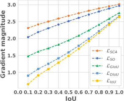
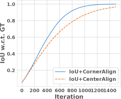
Figure 1: (left) The relationship between gradient magnitude and IoU. Gradient magnitude is the mean of $||\frac{\partial{\mathcal{L}}}{\partial{x}}||_{2}$ in different IoU intervals, where IoU interval = {[0., 0.1], [0.1, 0.2], …, [0.9, 1.0]}, $x=(x_{1},y_{1},x_{2},y_{2})$ is the bounding box corner point. The gradient of $\mathcal{L}_{IoU}$ significantly drops in low overlapping cases, but $\mathcal{L}_{SO}$, $\mathcal{L}_{SCA}$ still have a large gradient. All results are calculated with 1000k random boxes. (right) A comparison between center alignment and corner alignment. The loss weight of corner alignment is 0.5x as center alignment. Detail settings can be found in the Approach section.

1) Gradient vanish problem: IoU-based methods (IoU, GIoU, DIoU) improve baseline for high overlapping metric like AP75, but have relatively inferior performance in AP50. We further investigate this phenomenon and notice that IoU loss will lead to gradient vanish problem for non-overlapping cases and produce small gradient for low overlapping cases. In Fig. 1 (left), we visualize the relationship between gradient magnitude and IoU for different loss functions. It shows that lower IoU cases will have relatively smaller gradient value. During the training process, the small gradients produced by low overlapping boxes (hard samples) may be drowned into the large gradients by high overlapping ones (easy samples), thus limiting the overall performance. Since IoU is a component of GIoU and DIoU, they still encounter this problem. When predicted boxes lie within ground truth boxes, as shown in Fig. 2, all IoU value is the same and GIoU degrades into IoU. When the center of box is close to its ground truth, the normalized center distance in DIoU is near zero. In this case, the DIoU is roughly the same as IoU. For the aforementioned cases, GIoU and DIoU still produce small gradient, resulting in inferior performance.

2) Slow convergence speed: Although DIoU (Zheng et al. 2019) can speed up the convergence to a certain, the designed objective function is still not optimal. As DIoU discusses, GIoU tends to increase the size of box for non-overlapping cases until it has overlap with the ground truth box, which makes GIoU slow for convergence. Thus, DIoU adds a penalty term, i.e., the normalized center distance to directly “pull” closer boxes, which makes the DIoU converge faster than GIoU. However, as Fig. 2 shows, DIoU contributes little when the center of predicted box is near target box. In these cases, the corner distance is still far from the ground truth box. We further compare center alignment (regressing normalized center distance) with the corner alignment (regressing normalized corner distance) as shown in Fig. 1 (right). It illustrates the corner alignment converges faster than center alignment. Therefore, regressing the two corner points can be a better choice.

In this work, we propose Side and Corner Aligned Loss (SCALoss) to solve the shortcoming of IoUs and speed up the convergence. It is a combination of Side Overlap (SO) loss ($\mathcal{L}_{SO}$, Eq. (2)) and Corner Distance (CD) loss ($\mathcal{L}_{LD}$, Eq. (3)). The Side Overlap maximizes the side overlap of bounding boxes, which puts more penalty for low-overlapping cases and focuses more on hard samples. As shown in Fig. 1 (left), SO still keeps a large gradient in the low overlapping cases, while the gradient of IoU significantly drops. Furthermore, SO loss is well-correlated with IoU loss (see the Sec. Relationship with IoU and GIoU). Specifically, it can also benefit the evaluation metric (IoU). The Corner Distance adds the normalized corner distance to achieve accurate corner alignment and faster convergence speed. By incorporating the Side Overlap loss and Corner Distance loss, SCALoss can serve a more comprehensive similarity measure, leading the better localization performance and faster convergence speed.

To demonstrate the generality of SCALoss, we evaluate it with various CNN-based object detection frameworks including YOLOV3 (Redmon and Farhadi 2018), SSD (Liu et al. 2016), Faster R-CNN (Ren et al. 2015) on PASCAL VOC (Everingham et al. 2010), MS-COCO (Lin et al. 2014) , and LVIS (Gupta, Dollar, and Girshick 2019) datesets. Experimental results demonstrate that our approach achieves better object localization accuracy and gets consistent improvements.

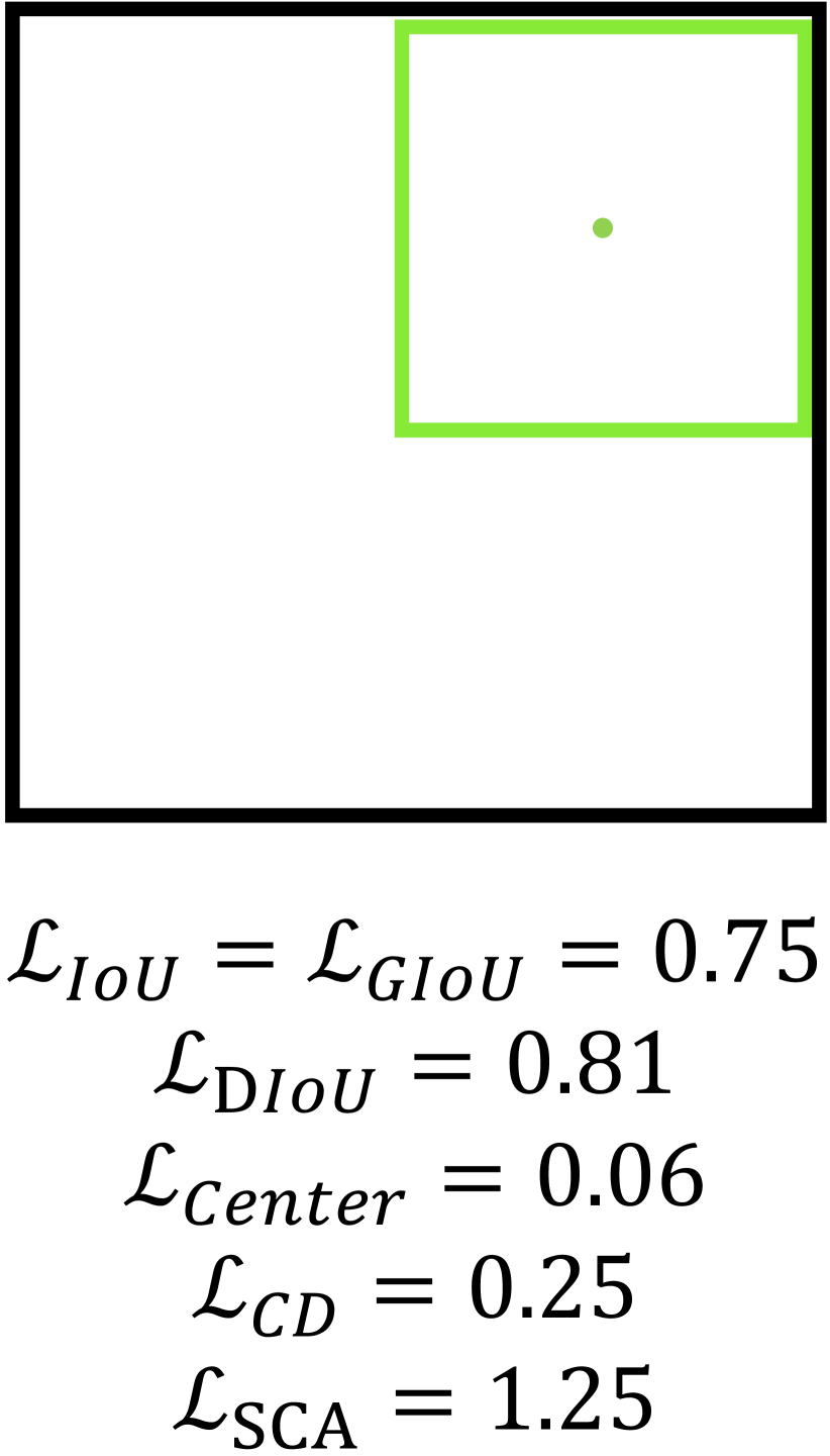
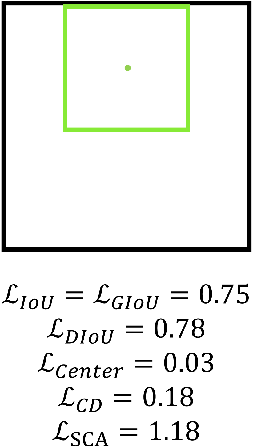
Figure 2: Green and black bounding box denote the predicted box and ground truth box respectively. $\mathcal{L}_{CD}$ is Eq.(3) and $\mathcal{L}_{Center}$ is the normalized center distance in DIoU. In thest cases, GIoU degrades into IoU and DIoU heavily relies IoU yielding inferior performance.

Our contributions can be summarized as follows:

• We show that IoU based method has the gradient problem for low overlapping bounding boxes and the normalized corner distance can speed up convergence.

• We propose SCALoss to evaluate the similarity of bounding boxes by using corner points and box sides, which outperforms $\ell_{n}$ loss and IoU-based loss (including IoU (Yu et al. 2016), GIoU (Rezatofighi et al. 2019), DIoU (Zheng et al. 2019), and CIoU (Zheng et al. 2019)). It can be easily plugged into any detection framework to achieve better localization accuracy.

• We experimentally demonstrate that SCALoss can achieve noticeable and consistent improvement with different detection frameworks on PASCAL VOC, COCO, and LVIS benchmarks.

Related Work

Object Detection

Current object detection methods can be roughly categorized into two classes: anchor-based detectors and anchor-free detectors. Anchor-based detectors can be divided into two-stage and one-stage methods.

Anchor-based Detectors

Anchor-based detectors consist of two-stage detectors and one-stage detectors. For two-stage detectors, R-CNN based methods (Girshick et al. 2014; Girshick 2015; Ren et al. 2015) generate object proposals with sliding window for second stage classifier as well as bounding box refinement. After that, lots of algorithms are proposed to improve its performance (Dai et al. 2016; Cai and Vasconcelos 2018; Shrivastava and Gupta 2016; Li et al. 2019; Lu et al. 2019). Compared to two-stage methods, the one-stage detectors directly predict bounding boxes and class scores without object proposal generation such as SSD (Liu et al. 2016) and YOLO series (Redmon et al. 2016; Redmon and Farhadi 2017, 2018; Bochkovskiy, Wang, and Liao 2020; Wang, Bochkovskiy, and Liao 2020). Thereafter, plenty of works are presented to boost its performance(Fu et al. 2017; Kong et al. 2017; Zhang et al. 2018). These methods are superior in inference speed but inferior in accuracy compared to two-stage methods. Among these methods, Focal loss (Lin et al. 2017) solves the problem of extreme foreground-background class imbalance. Generally, one-stage method is considered to be promising to achieve similar accuracy with two-stage method.

Anchor-free Detectors

Anchor-free detectors mainly locate several pre-defined keypoints and generate bounding boxes to detect objects. CornerNet (Law and Deng 2018) detects an object bounding box as a pair of keypoints while CenterNet (Duan et al. 2019) detects object center and regress the size of the object. ExtremeNet (Zhou, Zhuo, and Krahenbuhl 2019) detects four extreme points and one center to generate the object bounding box. Reppoints (Yang et al. 2019) represents objects as a set of sample points to adaptively position themselves over an object and utilizes deformable convolution (Zhu et al. 2019) to get more accurate features. These anchor-free detectors are able to eliminate those hyper-parameters related to anchors and have achieved similar performance with anchor-based detectors.

Bounding Box Regression Loss

Various bounding box regression losses have been proposed in recent years. $\ell_{1}$-smooth loss (Girshick 2015) proposes to combine $\ell_{1}$ loss and $\ell_{2}$ loss so that the loss is less sensitive to outliers and more stable for inliers. Balanced L1 loss (Pang et al. 2019) proposes to promote the crucial regression gradients (inliers) for the balance between classification and localization. Bounded IoU loss (Tychsen-Smith and Petersson 2018) derives a novel bounding box regression loss based on a set of IoU upper bounds that better matches the goal of IoU maximization while still providing good convergence properties. KLLoss (He et al. 2019) proposes a bounding box regression loss for learning bounding box transformation and localization variance together. The learned localization variance can merge neighboring bounding boxes during non-maximum suppression (NMS), which further improves the localization performance. UnitBox (Yu et al. 2016) first proposes IoU Loss for object detection, which regresses the bounding box as a whole unit. GIoU (Rezatofighi et al. 2019) discusses the weakness of IoU for the case of non-overlapping bounding boxes and introduces a generalized version of IoU as a new loss. DIoU (Zheng et al. 2019) adds the normalized center distance between the predicted and the target box on IoU loss, which helps converge faster in training. CIoU (Zheng et al. 2019) suggests the consistency of aspect ratios for bounding boxes is also an important geometric factor and extends DIoU by regressing aspect ratios, leading to better performance.

Approach

In this section, we first introduce our Side and Corner Aligned loss for bounding box regression, then we analyze the SO loss and compare it with IoU based loss.

Side and Corner Aligned Loss

Following (He et al. 2019), we regress the corners of a bounding box separately. We adopt the parameter of the $(x_{1},y_{1},x_{2},y_{2})\in\mathcal{R}^{4}$ coordinate as bounding box representation, where $(x_{1},y_{1})$, $(x_{2},y_{2})$ are top left and bottom right corner respectively. Our loss function includes side overlap (SO) and corner distance (CD) two parts.

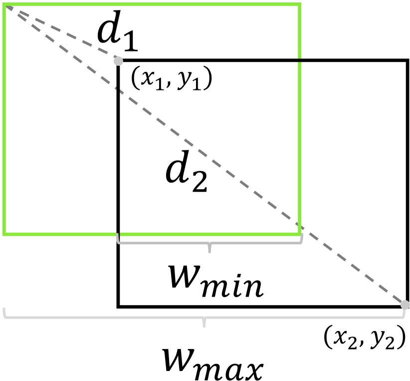
(a) Overlapping case

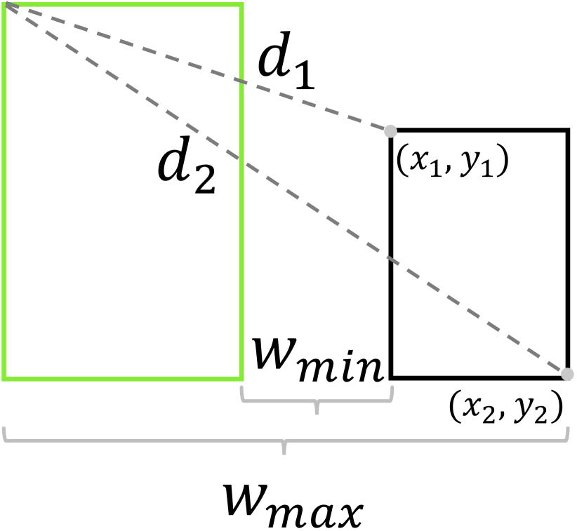
(b) Non-overlapping case

Figure 3: Side and Corner Align loss for the bounding box regression. It directly regresses two corner points by minimizing the normalized distance $\frac{d_{1}}{d_{2}}$ and enlarges width by minimizing the $1-\frac{w_{min}}{w_{max}}$. We omit the another corner and side for simplicity.

Side Overlap

We propose Side Overlap (SO) loss to measure bounding box similarity by maximizing the overlap of width and height. It is a stricter constraint and puts more gradient for low overlapping bounding box. As shown in Fig. 3, given the predicted box ($x_{1},x_{2},y_{1},y_{2}$) and ground truth box ($x_{1}^{g},y_{1}^{g},x_{2}^{g},y_{2}^{g}$), the SO loss simultaneously maximizes the overlap for both sides of a predicted box with its ground truth. SO is defined as follows:

$$SO=\frac{w_{min}}{w_{max}}+\frac{h_{min}}{h_{max}},$$ (1)

where $w_{min}=\min(x_{2},x_{2}^{g})-\max(x_{1},x_{1}^{g})$, $w_{max}=\max(x_{2},x_{2}^{g})-\min(x_{1},x_{1}^{g})$, $h_{min}=\min(y_{2},y_{2}^{g})-\max(y_{1},y_{1}^{g})$, $h_{max}=\max(y_{2},y_{2}^{g})-\min(y_{1},y_{1}^{g})$. Note $w_{min}$, $h_{min}$ may be negative when bounding boxes are non-overlapping as shown in Fig. 3(b). Thus, SO loss can also be optimized for non-overlapping cases. The SO loss can be formulated as follows:

$$\mathcal{L}_{SO}=2-SO.$$ (2)

Corner Distance

Furthermore, we introduce Corner Distance (CD) loss to achieve better corner alignment. As shown in Fig. 2, the normalized center distance in DIoU is roughly near zero in these cases, but the corner point still misaligns. Therefore, we add CD in the loss to achieve accurate box regression. The CD directly minimizes the normalized corner distance. It is defined as follows:

$$\mathcal{L}_{CD}=\frac{D(p_{1},p_{1}^{g})}{D(p_{c_{1}},p_{c_{2}})}+\frac{D(p_{2},p_{2}^{g})}{D(p_{c_{1}},p_{c_{2}})},$$ (3)

where $D(\cdot,\cdot)$ is the Euclidean distance, $p_{1}$, $p_{2}$ denote the top left and bottom right corner points of predicted box, $p_{1}^{g}$, $p_{2}^{g}$ are corresponding ground truth points, $p_{c_{1}}$, $p_{c_{2}}$ are corner points of the smallest enclosing box covering two boxes.

The final SCALoss can be formulated as follows:

$$\mathcal{L}_{SCA}=\mathcal{L}_{SO}+\alpha\mathcal{L}_{CD},$$ (4)

where $\alpha$ is the weight factor, and $\alpha$ is set to 0.5 in our experiment.

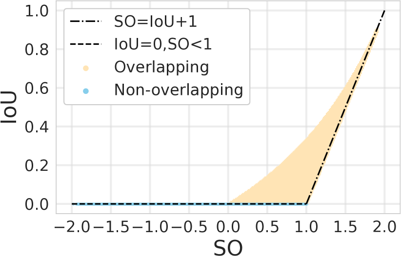
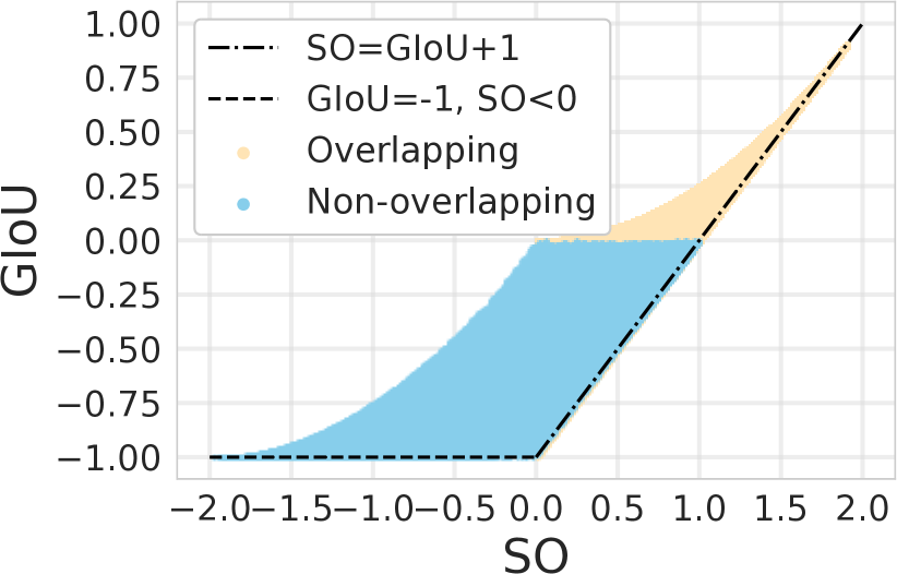
Figure 4: (left) Relationship between IoU and SO, (right) Relationship between GIoU and SO for overlapping and non-overlapping samples.

Relationship with IoU and GIoU

For two arbitrary axis-aligned bounding boxes $A,B\in\mathcal{R}^{4}$, we can calculate the SO, IoU, and GIoU by their definitions respectively. The SO has the following properties:

• Similar to IoU and GIoU, SO is invariant to the scale of the problem. Because the loss is normalized by the scale of box.

• SO is always a lower bound for $IoU+1$ and $GIoU+1$, and this lower bound becomes tighter when A and B have a stronger shape similarity.

• $\forall A,B\in\mathcal{R}^{4}$, $0\leq IoU(A,B)\leq 1$, SO and GIoU have a symmetric range, $\forall A,B\in\mathcal{R}^{4}$, $-1\leq GIoU(A,B)\leq 1$, $-2\leq SO(A,B)\leq 2$.

  • Similar to IoU and GIoU, the max value occurs when two objects match perfectly, i.e. if $|A\cup B|=|A\cap B|$, then SO = 2, IoU = GIoU = 1.

  • SO value asymptotically converges to -2 when two bounding boxes are far away.

• Different from IoU, SO still has gradient for non-overlaps cases and it has a larger gradient than GIoU.

We also demonstrate this correlation qualitatively in Fig. 4 by taking over samples from 1000K random samples from coordinates of two 2D rectangles. It shows that SO has a strong correlation with IoU and GIoU in high IoU values. However, in the case of low overlapping, SO can make the bounding box change position and shape faster compared with IoU and GIoU. Thus, SO is promising to have a larger gradient in these cases. In conclusion, optimizing SO loss can be a better choice than optimizing IoU and GIoU loss.

Simulation Experiment

To better understand the efficiency of our $\mathcal{L}_{SCA}$, we also provide a simple simulation experiment to compare $\mathcal{L}_{IoU}$, $\mathcal{L}_{GIoU}$, and $\mathcal{L}_{DIoU}$. In the simulation experiment, we try to enumerate all possible anchor boxes. In particular, we choose 5 specific boxes with different aspect ratios (e.g. 4:1, 2:1, 1:1, 1:2, 1:4) as ground truth boxes. Then anchor boxes are uniformly sampled in $20\times 20$ grid with the ratio of (2:1, 1:1, 1:2) and scale of (2, 4, 6) and thus we have 3600 anchors as we can see in Fig. 5(a). All the anchor boxes should be regressed to each ground truth box. Different with DIoU (Zheng et al. 2019), most boxes have overlap with their ground truth in our setting. Therefore, the simulation experiment is more similar to the real training procedure.

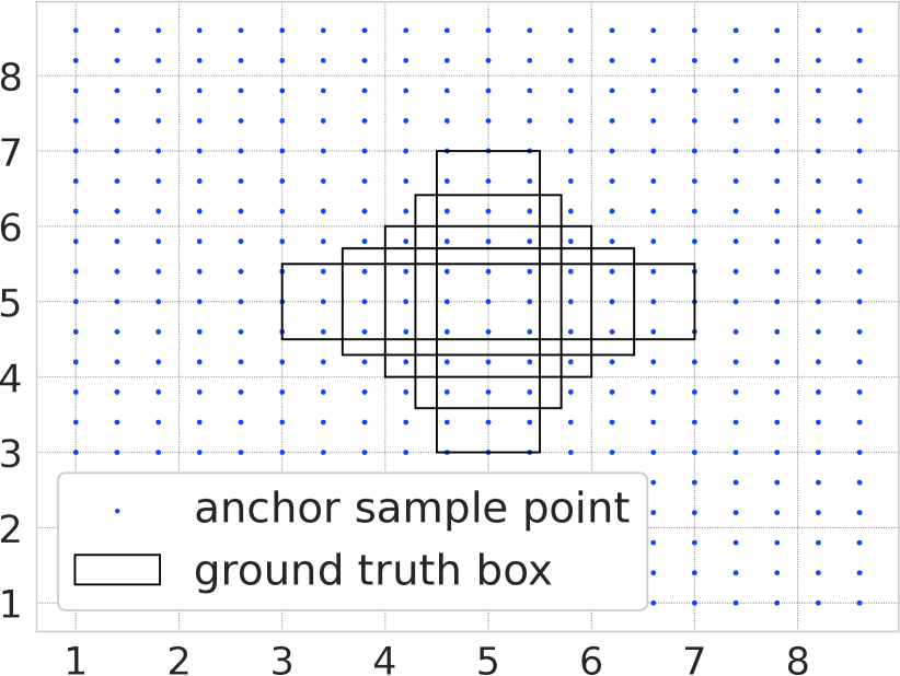
(a) anchors setting

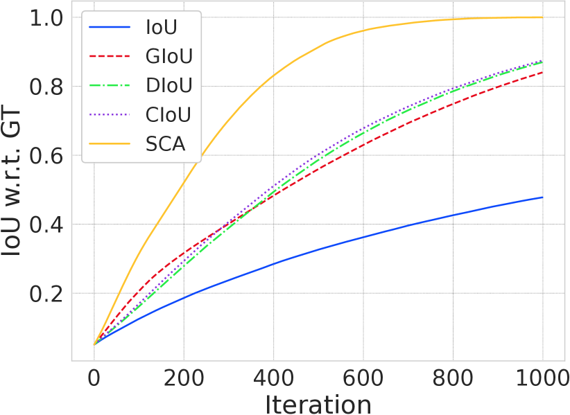
(b) regression results

Figure 5: (a) 3600 regression anchor boxes are adopted by considering different scales and aspect ratios, (b) regression results curves with iteration t of different bounding box regression losses.

Given a loss function $\mathcal{L}$, we can simulate the procedure of bounding box regression using gradient descent algorithm. For each predicted box, we first calculate the loss function and the gradient:

$$Loss=\mathcal{L}(B^{t},B_{gt}),$$ (5)

$$\nabla B^{t}=\frac{\partial Loss}{\partial B^{t}},$$ (6)

Then, the update process can be obtained by:

$$B^{t}=B^{t-1}+\eta\nabla B^{t-1}.$$ (7)

where $\eta$ is the learning rate, $B^{t}$ is the predicted box at iteration $t$ and $\nabla B^{t}$ is the gradient of the corresponding box. Finally, we calculate the mean IoU to evaluate the regression accuracy with different loss functions. The final regression result has shown in Fig. 5(b).

SCALoss can converge faster from the results in Fig. 5(b) because it produces large gradient for low overlapping boxes as we discuss in Sec. Introduction. This demonstrates SCALoss is a stricter similarity measure, and evaluating the similarity of corners and sides is more efficient in accurating bounding box regression.

Experiment

In this section, we construct experiments to evaluate the performance of our SCALoss by incorporating it into the most popular object detectors such as YOLOV3, SSD, Faster R-CNN. To this end, we replace their default regression losses with $\mathcal{L}_{SCA}$, i.e., we replace $\ell_{n}$ loss in YOLOV3 / SSD / Faster R-CNN. We compare $\mathcal{L}_{SCA}$ against $\mathcal{L}_{IoU}$, $\mathcal{L}_{GIoU}$, $\mathcal{L}_{DIoU}$, and $\mathcal{L}_{CIoU}$. We use the mmdetection (Chen et al. 2019) toolbox to conduct all our experiments except YOLOV3. We use Pytorch (Paszke et al. 2019) with the NVIDIA 1080Ti GPU in Ubuntu. All models are pre-trained on ImageNet (Deng et al. 2009).

Dataset

All results are reported on three popular object detection benchmarks, the PASCAL VOC, MS-COCO, and LVIS.
PASCAL VOC: The Pascal Visual Object Classes (VOC) dataset is one of the most popular benchmarks for category classification, detection, and semantic segmentation. For object detection, it has 20 pre-defined classes with annotated bounding boxes. We use PASCAL VOC 2007 + 2012 (the union of VOC 2007 and VOC 2012 trainval) with 16551 images as the training set and PASCAL VOC 2007 test with 4952 images as the test set.
MS COCO: Microsoft Common Objects in Context (MS-COCO) is another popular dataset for object detection, instance segmentation, and object keypoint detection. It is a large scale dataset with 80 pre-defined classes. We use COCO train2017 with 135k images as the training set, val2017 with 5k images as the validation set and test-dev with 20k images as the test set.
LVIS: LVIS is a large vocabulary dataset for instance segmentation, which contains 1203 categories in current version v1.0. In LVIS, categories are divided into three groups according to the number of images that contains those categories: rare (1-10 images), common (11-100), and frequent ($>$100). We train our model on 57k train images and evaluate it on 20k val set.

Evaluation

In this paper, we adopt the same mAP calculation method as MS COCO to report all our results. The mAP score is calculated by taking mean AP over all classes and over all 10 IoU thresholds, i.e. IoU= 0.5, 0.55, …, 0.95. While PASCAL VOC only considers one IoU, i.e., IoU = 0.5, we modify it same as COCO for better performance comparison. For LVIS, we also report the $AP_{r},AP_{c},AP_{f}$ for rate, common, and frequent categories respectively.

YOLOV3 and SSD

We first use two representative one-stage detectors, i.e., YOLOV3 and SSD, to construct experiments.

YOLOV3-tiny on COCO

Following its training protocol, we train YOLOV3-tiny with every aforementioned bounding box regression loss on the training set for 300 epochs. The input image size is $640\times 640$. We show the performance of each loss in Table YOLOV3 on COCO. The result shows that training YOLOV3-tiny with $\mathcal{L}_{SCA}$ can considerably improve its performance, near 1 AP, compared to $\mathcal{L}_{IoU}$, $\mathcal{L}_{GIoU}$, $\mathcal{L}_{DIoU}$, and $\mathcal{L}_{CIoU}$. Note that the improvement mostly comes from high overlap metrics, e.g., near 1.8 points in AP75. Our method promotes the gradient for low overlapping cases, so the APs from low overlap metrics (like AP50, AP65) are much better than $\mathcal{L}_{IoU}$, $\mathcal{L}_{GIoU}$, $\mathcal{L}_{DIoU}$, and $\mathcal{L}_{CIoU}$.

We also plot the relationship between training epoch and mAP, as we can see in Fig. 6, our SCALoss can converge faster than other losses and get consistent higher AP during the training process.

YOLOV3 on COCO

Similarly, we train YOLOV3 using each of aforementioned bounding box regression losses on COCO dataset. The backbone is darknet-53 and other settings are same as YOLOv3-tiny. As Table YOLOV3 on COCO shows, SCALoss can also surpass other losses consistently for the higher baseline models.

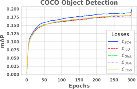
Figure 6: mAP value against train epochs for YOLO-tiny using $\mathcal{L}_{GIoU}$, $\mathcal{L}_{DIoU}$, and $\mathcal{L}_{SCA}$ on COCO 2017 val set.

tabularc c c c c c c @Loss @mAP @AP₅₀ @ AP₆₅ @ AP₇₅ @ AP₈₀ @AP₉₀
$@\mathcal{L}_{IoU}$ 18.8 36.2 27.2 17.3 11.6 1.9
$@\mathcal{L}_{GIoU}$ 18.8 36.2 27.1 17.6 11.8 2.1
@rela. improv. :=round((b3-b2)/b2*100,2)% :=round((c3-c2)/c2*100,2)% :=round((d3-d2)/d2*100,2)% :=round((e3-e2)/e2*100,2)% :=round((f3-f2)/f2*100,2)% :=round((g3-g2)/g2*100,2)%
$@\mathcal{L}_{DIoU}$ 18.8 36.4 26.9 17.2 11.8 1.9
@rela. improv. :=round((b5-b2)/b2*100,2)% :=round((c5-c2)/c2*100,2)% :=round((d5-d2)/d2*100,2)% :=round((e5-e2)/e2*100,2)% :=round((f5-f2)/f2*100,2)% :=round((g5-g2)/g2*100,2)%
$@\mathcal{L}_{CIoU}$ 18.9 36.6 27.3 17.2 11.6 2.1
@rela. improv. :=round((b7-b2)/b2*100,2)% :=round((c7-c2)/c2*100,2)% :=round((d7-d2)/d2*100,2)% :=round((e7-e2)/e2*100,2)% :=round((f7-f2)/f2*100,2)% :=round((g7-g2)/g2*100,2)%
$@\mathcal{L}_{SCA}$ ¿19.9 ¿36.6 ¿28.3 ¿19.1 ¿13.3 ¿2.7
@rela. improv. :=round((b9-b2)/b2*100,2)% :=round((c9-c2)/c2*100,2)% :=round((d9-d2)/d2*100,2)% :=round((e9-e2)/e2*100,2)% :=round((f9-f2)/f2*100,2)% :=round((g9-g2)/g2*100,2)%

Table 1: Comparison between the performance of YOLOV3-tiny trained using $\mathcal{L}_{IoU}$, $\mathcal{L}_{GIoU}$, $\mathcal{L}_{DIoU}$, $\mathcal{L}_{CIoU}$, and $\mathcal{L}_{SCA}$ losses on COCO 2017 val set.

tabularc c c c c c c @Loss @mAP @AP₅₀ @ AP₆₅ @ AP₇₅ @ AP₈₀ @AP₉₀
$@\mathcal{L}_{IoU}$ 44.8 64.2 57.5 48.8 41.8 20.7
$@\mathcal{L}_{GIoU}$ 44.7 ¿64.4 57.5 48.5 42.0 20.4
@rela. improv. :=round((b3-b2)/b2*100,2)% :=round((c3-c2)/c2*100,2)% :=round((d3-d2)/d2*100,2)% :=round((e3-e2)/e2*100,2)% :=round((f3-f2)/f2*100,2)% :=round((g3-g2)/g2*100,2)%
$@\mathcal{L}_{DIoU}$ 44.7 64.3 57.5 48.9 42.1 19.8
@rela. improv. :=round((b5-b2)/b2*100,2)% :=round((c5-c2)/c2*100,2)% :=round((d5-d2)/d2*100,2)% :=round((e5-e2)/e2*100,2)% :=round((f5-f2)/f2*100,2)% :=round((g5-g2)/g2*100,2)%
$@\mathcal{L}_{CIoU}$ 44.7 64.3 57.5 48.9 41.7 19.8
@rela. improv. :=round((b7-b2)/b2*100,2)% :=round((c7-c2)/c2*100,2)% :=round((d7-d2)/d2*100,2)% :=round((e7-e2)/e2*100,2)% :=round((f7-f2)/f2*100,2)% :=round((g7-g2)/g2*100,2)%
$@\mathcal{L}_{SCA}$ ¿45.3 64.1 ¿57.9 ¿49.9 ¿43.3 ¿21.4
@rela. improv. :=round((b9-b2)/b2*100,2)% :=round((c9-c2)/c2*100,2)% :=round((d9-d2)/d2*100,2)% :=round((e9-e2)/e2*100,2)% :=round((f9-f2)/f2*100,2)% :=round((g9-g2)/g2*100,2)%

Table 2: Comparison between the performance of YOLOV3 trained using $\mathcal{L}_{IoU}$, $\mathcal{L}_{GIoU}$, $\mathcal{L}_{DIoU}$, $\mathcal{L}_{CIoU}$, and $\mathcal{L}_{SCA}$ losses on COCO 2017 val set.

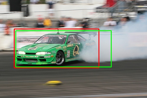
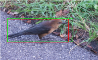
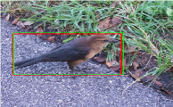
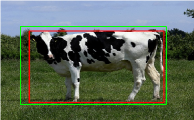
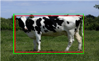
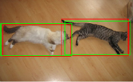
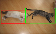
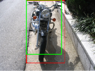
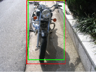
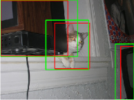
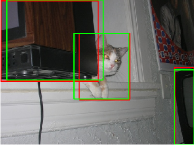
Figure 7: Examples results from PASCAL VOC dataset using Faster R-CNN trained with $\mathcal{L}_{GIoU}$ and $\mathcal{L}_{SCA}$ (left to right). Red: the ground truth box, green: the predicted box.

SSD on PASCAL VOC

When training SSD on PASCAL VOC, we use the same setting as the COCO. The training epochs is 72. The performance for each loss has been shown in Table SSD on PASCAL VOC. The result shows that training SSD with $\mathcal{L}_{SCA}$ can considerably improve its performance compared to $\mathcal{L}_{IoU}$. Moreover, $\mathcal{L}_{SCA}$ can get better performance than $\mathcal{L}_{GIoU}$, and $\mathcal{L}_{DIoU}$.

tabularc c c c c c c @Loss @mAP @AP₅₀ @ AP₆₅ @ AP₇₅ @ AP₈₀ @AP₉₀
@$\mathcal{L}_{IoU}$ 52.28 78.26 68.51 56.22 46.90 20.20
@$\mathcal{L}_{GIoU}$ 52.50 78.57 69.11 56.71 46.87 19.88
@rela. improv. :=round((b3-b2)/b2*100,2)% :=round((c3-c2)/c2*100,2)% :=round((d3-d2)/d2*100,2)% :=round((e3-e2)/e2*100,2)% :=round((f3-f2)/f2*100,2)% :=round((g3-g2)/g2*100,2)%
@$\mathcal{L}_{DIoU}$ 52.65 78.64 69.11 56.55 47.9 20.09
@rela. improv. :=round((b5-b2)/b2*100,2)% :=round((c5-c2)/c2*100,2)% :=round((d5-d2)/d2*100,2)% :=round((e5-e2)/e2*100,2)% :=round((f5-f2)/f2*100,2)% :=round((g5-g2)/g2*100,2)%
@$\mathcal{L}_{CIoU}$ 52.75 78.76 69.03 56.45 48.56 20.69
@rela. improv. :=round((b7-b2)/b2*100,2)% :=round((c7-c2)/c2*100,2)% :=round((d7-d2)/d2*100,2)% :=round((e7-e2)/e2*100,2)% :=round((f7-f2)/f2*100,2)% :=round((g7-g2)/g2*100,2)%
@$\mathcal{L}_{SCA}$ ¿53.45 ¿78.82 ¿69.17 ¿57.22 ¿48.49 ¿22.67
@rela. improv. :=round((b9-b2)/b2*100,2)% :=round((c9-c2)/c2*100,2)% :=round((d9-d2)/d2*100,2)% :=round((e9-e2)/e2*100,2)% :=round((f9-f2)/f2*100,2)% :=round((g9-g2)/g2*100,2)%

Table 3: Comparison between the performance of SSD trained using $\mathcal{L}_{IoU}$, $\mathcal{L}_{GIoU}$, $\mathcal{L}_{DIoU}$, $\mathcal{L}_{CIoU}$, and $\mathcal{L}_{SCA}$ losses on the PASCAL VOC 2007 test set.

Faster R-CNN

Faster R-CNN is a two-stage detector, which generates object proposals for the second stage to classify and refine bounding boxes. We use the ResNet50-FPN backbone network and replace the $\ell_{1}$-smooth loss in the second stage in Faster R-CNN.

Faster R-CNN on PASCAL VOC

We train Faster R-CNN for 12 epochs on PASCAL VOC dataset, and the input image is resized to $1000\times 600$. The final results have been reported in Table Faster R-CNN on PASCAL VOC. The results show that training Faster-RCNN using our SCALoss can consistently improve its performance compared to IoU loss (near 2%). SCALoss can improve the performance with gains of near 0.9 AP / 0.8 AP than GIoU loss, CIoU loss respectively.

Fig. 7 shows the qualitative results of models trained using GIoU loss and SCA loss. Adopting SCA loss can get more accurate bounding boxes than GIoU loss and the corners of bounding boxes can be regressed better, which demonstrates SCA can better align the bounding box and yield a better detection performance.

tabularc c c c c c c @Loss @mAP @AP₅₀ @ AP₆₅ @ AP₇₅ @ AP₈₀ @AP₉₀
@ $\mathcal{L}_{IoU}$ 50.85 79.60 69.85 55.14 43.23 13.01
@ $\mathcal{L}_{GIoU}$ 50.90 79.69 70.56 55.00 43.34 12.70
@ rela. improv. :=round((b3-b2)/b2*100,2)% :=round((c3-c2)/c2*100,2)% :=round((d3-d2)/d2*100,2)% :=round((e3-e2)/e2*100,2)% :=round((f3-f2)/f2*100,2)% :=round((g3-g2)/g2*100,2)%
@ $\mathcal{L}_{DIoU}$ 50.86 79.99 70.48 54.56 42.79 12.80
@ rela. improv. :=round((b5-b2)/b2*100,2)% :=round((c5-c2)/c2*100,2)% :=round((d5-d2)/d2*100,2)% :=round((e5-e2)/e2*100,2)% :=round((f5-f2)/f2*100,2)% :=round((g5-g2)/g2*100,2)%
@ $\mathcal{L}_{CIoU}$ 51.08 79.52 70.07 55.12 44.04 13.10
@ rela. improv. :=round((b7-b2)/b2*100,2)% :=round((c7-c2)/c2*100,2)% :=round((d7-d2)/d2*100,2)% :=round((e7-e2)/e2*100,2)% :=round((f7-f2)/f2*100,2)% :=round((g7-g2)/g2*100,2)%
@ $\mathcal{L}_{SCA}$ ¿51.84 ¿80.21 ¿70.91 ¿56.18 ¿45.14 ¿13.77
@rela. improv. :=round((b9-b2)/b2*100,2)% :=round((c9-c2)/c2*100,2)% :=round((d9-d2)/d2*100,2)% :=round((e9-e2)/e2*100,2)% :=round((f9-f2)/f2*100,2)% :=round((g9-g2)/g2*100,2)%

Table 4: Comparison between the performance of Faster-RCNN trained using $\mathcal{L}_{IoU}$, $\mathcal{L}_{GIoU}$, $\mathcal{L}_{DIoU}$, $\mathcal{L}_{CIoU}$, and $\mathcal{L}_{SCA}$ losses on the PASCAL VOC 2007 test set.

tabularc c c c c c c c c c @Loss @mAP @AP₅₀ @ AP₇₅ @ AP_s @AP_m @AP_l @AP_r @AP_c @AP_f
@ $\mathcal{L}_{IoU}$ 16.7 29.4 16.2 13.1 22.6 26.3 3.8 14.2 25.1
@ $\mathcal{L}_{GIoU}$ :=round(17.00009/1.0, 3) 29.1 17.2 round(13.0, 3) 23.3 26.7 4.4 14.4 25.3
@relative improv.(%) :=round((b3-b2)/b2*100,2)% :=round((c3-c2)/c2*100,2)% :=round((d3-d2)/d2*100,2)% :=round((e3-e2)/e2*100,2)% :=round((f3-f2)/f2*100,2)% :=round((g3-g2)/g2*100,2)% :=round((h3-h2)/h2*100,2)% :=round((i3-i2)/i2*100,2)% :=round((j3-j2)/j2*100,2)%
@ $\mathcal{L}_{DIoU}$ 16.8 29.5 16.6 13.3 round(23.2, 3) 26.2 3.3 14.5 25.2
@relative improv.(%) :=round((b5-b2)/b2*100,2)% :=round((c5-c2)/c2*100,2)% :=round((d5-d2)/d2*100,2)% :=round((e5-e2)/e2*100,2)% :=round((f5-f2)/f2*100,2)% :=round((g5-g2)/g2*100,2)% :=round((h5-h2)/h2*100,2)% :=round((i5-i2)/i2*100,2)% :=round((j5-j2)/j2*100,2)%
@ $\mathcal{L}_{CIoU}$ 16.7 29.5 16.5 13.2 23.2 26.1 3.3 14.3 25.3
@relative improv.(%) :=round((b7-b2)/b2*100,2)% :=round((c7-c2)/c2*100,2)% :=round((d7-d2)/d2*100,2)% :=round((e7-e2)/e2*100,2)% :=round((f7-f2)/f2*100,2)% :=round((g7-g2)/g2*100,2)% :=round((h7-h2)/h2*100,2)% :=round((i7-i2)/i2*100,2)% :=round((j7-j2)/j2*100,2)%
@ $\mathcal{L}_{SCA}$ ¿17.7 ¿30.4 ¿18. ¿13.5 ¿24.1 ¿28.3 ¿4.9 ¿15.4 ¿25.9
@relative improv.(%) :=round((b9-b2)/b2*100,2)% :=round((c9-c2)/c2*100,2)% :=round((d9-d2)/d2*100,2)% :=round((e9-e2)/e2*100,2)% :=round((f9-f2)/f2*100,2)% :=round((g9-g2)/g2*100,2)% :=round((h9-h2)/h2*100,2)% :=round((i9-i2)/i2*100,2)% :=round((j9-j2)/j2*100,2)%

Table 5: Comparison between the performance of Faster R-CNN trained using $\mathcal{L}_{IoU}$, $\mathcal{L}_{GIoU}$, $\mathcal{L}_{DIoU}$, $\mathcal{L}_{CIoU}$, and $\mathcal{L}_{SCA}$ losses on the LVIS1.0 val set.

Faster R-CNN on LVIS

Similarly, we train Faster R-CNN on the LVIS1.0 dataset using the aforementioned bounding box regression losses for 6 epochs, and training images are resized such that its shorter edge is 800 pixels while the longer edge is no more than 1333. The results are shown in Table Faster R-CNN on PASCAL VOC. We can observe that the SCA loss surpasses existing losses consistently in terms of mAP and $AP_{75}$ compared with other IoU-based losses. To be more specific, SCA achieves 1.0 point mAP and 1.8 point $AP_{75}$ higher than IoU loss, respectively. The superiority of SCA loss is more pronounced at high accuracy levels, which reach 11% relative improvement at AP75. The improvements of SCA loss mostly come all frequent categories, i.e., it improves 1.1 point $AP_{r}$, 1.2 points $AP_{c}$, and 1.1 points $AP_{f}$ comparing with IoU loss, respectively.

	IoU	Center Distance	SO	Corner Distance	mAP
(a)		✓			19.17
(b)				✓	52.64
(c)	✓				52.28
(d)	✓	✓			52.65
(e)	✓			✓	52.97
(f)			✓		53.07
(g)			✓	✓	53.45

Table 6: The contributions of the proposed components on PASCAL VOC test set with SSD.

Ablation Study of Each Loss Item

In this section, we conduct the experiments on PASCAL VOC with SSD to clarify the contributions of the proposed Corner Distance (CD) loss, Side Overlap (SO) loss, and the results are shown in Table 6. Firstly, Side Overlap and Corner Distance can be separate as a loss while Center Distance cannot (see (a), (b), and (f)). In the same time, Corner Distance with IoU loss can be more powerful than Center Distance with IoU loss (DIoU loss), comparing the (d) and (e). Furthermore, CD loss can achieve the better performance than IoU loss (see (b) and (c)). Secondly, SO loss can bring substantial improvement than IoU loss (+0.8 mAP, (c) and (f)). Finally, the overall performance is +1.2mAP than the IoU, which shows the superiority of our SCALoss.

Ablation Study of Weight Factor $\alpha$

In this section, we study the weight factor $\alpha$ for $\mathcal{L}_{SO}$ and $\mathcal{L}_{CD}$ in Eq. (4). We use the SSD detection framework and the PASCAL VOC dataset to conduct experiments. The input image is resized to $300\times 300$. We replace the $\ell_{1}$-smooth with our SCALoss and use different $\alpha=\{0.2,0.3,...,0.7\}$ to show the importance of this parameter. The results have been shown in Table 7.

For different models and datasets, we can make efforts to search an optimal $\alpha$ for better performance. However, for simplicity and saving computational resources, we choose $\alpha=0.5$ for all our settings.

$\alpha$	mAP	AP50	AP65	AP75	AP80	AP90
0.2	53.23	79.05	69.29	57.01	48.91	21.56
0.3	53.26	78.38	69.35	57.63	49.06	21.24
0.4	53.34	78.59	69.23	58.01	49.25	21.54
0.5	53.45	78.82	69.17	57.22	48.49	22.67
0.6	53.33	78.51	69.26	57.33	48.02	22.81
0.7	53.23	78.39	68.93	57.21	48.77	21.87

Table 7: Study for different weight factor $\alpha$ for SSD trained using $\mathcal{L}_{SCA}$ on the PASCAL VOC 2007 test set.

Conclusions

In this paper, we propose Side and Corner Aligned Loss (SCALoss) for bounding box regression. SCALoss consists of Side Overlap and Corner Distance, which takes bounding box side and corner points into account. Combine the advantage of these two parts, SCALoss not only produces more penalty for low overlapping boxes and focuses more on hard samples but also speeds up the model convergence. In a result, SCALoss can serve as a more comprehensive measure than $\ell_{n}$ loss and IoU-based loss. Experiments on COCO, PASCAL VOC, and LVIS benchmarks show that SCALoss can bring consistent improvement and outperform $\ell_{n}$ loss and IoU based loss with popular object detectors, such as YOLOV3, SSD, and Faster R-CNN.

In the future, we plan to investigate the feasibility of deriving an extension for SCALoss in the case of 3D object detection. This extension is promising to improve the performance of 3D object detection.

Acknowledgments

This work was supported in part by The National Key Research and Development Program of China (Grant Nos: 2018AAA0101400), in part by The National Nature Science Foundation of China (Grant Nos: 62036009, 61936006), in part by Innovation Capability Support Program of Shaanxi (Program No. 2021TD-05).

References

- Bochkovskiy, Wang, and Liao (2020) Bochkovskiy, A.; Wang, C.-Y.; and Liao, H.-Y. M. 2020. Yolov4: Optimal speed and accuracy of object detection. arXiv preprint arXiv:2004.10934.
- Cai and Vasconcelos (2018) Cai, Z.; and Vasconcelos, N. 2018. Cascade r-cnn: Delving into high quality object detection. In Proceedings of the IEEE conference on computer vision and pattern recognition, 6154–6162.
- Chen et al. (2019) Chen, K.; Wang, J.; Pang, J.; Cao, Y.; Xiong, Y.; Li, X.; Sun, S.; Feng, W.; Liu, Z.; Xu, J.; et al. 2019. MMDetection: Open MMLab Detection Toolbox and Benchmark. arXiv preprint arXiv:1906.07155.
- Dai et al. (2016) Dai, J.; Li, Y.; He, K.; and Sun, J. 2016. R-fcn: Object detection via region-based fully convolutional networks. In Advances in neural information processing systems, 379–387.
- Deng et al. (2009) Deng, J.; Dong, W.; Socher, R.; Li, L.-J.; Li, K.; and Fei-Fei, L. 2009. Imagenet: A large-scale hierarchical image database. In 2009 IEEE conference on computer vision and pattern recognition, 248–255. Ieee.
- Duan et al. (2019) Duan, K.; Bai, S.; Xie, L.; Qi, H.; Huang, Q.; and Tian, Q. 2019. Centernet: Keypoint triplets for object detection. In Proceedings of the IEEE International Conference on Computer Vision, 6569–6578.
- Everingham et al. (2010) Everingham, M.; Van Gool, L.; Williams, C. K.; Winn, J.; and Zisserman, A. 2010. The pascal visual object classes (voc) challenge. International journal of computer vision, 88(2): 303–338.
- Fu et al. (2017) Fu, C.-Y.; Liu, W.; Ranga, A.; Tyagi, A.; and Berg, A. C. 2017. Dssd: Deconvolutional single shot detector. arXiv preprint arXiv:1701.06659.
- Girshick (2015) Girshick, R. 2015. Fast r-cnn. In Proceedings of the IEEE international conference on computer vision, 1440–1448.
- Girshick et al. (2014) Girshick, R.; Donahue, J.; Darrell, T.; and Malik, J. 2014. Rich feature hierarchies for accurate object detection and semantic segmentation. In Proceedings of the IEEE conference on computer vision and pattern recognition, 580–587.
- Gupta, Dollar, and Girshick (2019) Gupta, A.; Dollar, P.; and Girshick, R. 2019. LVIS: A dataset for large vocabulary instance segmentation. In Proceedings of the IEEE/CVF Conference on Computer Vision and Pattern Recognition, 5356–5364.
- He et al. (2017) He, K.; Gkioxari, G.; Dollár, P.; and Girshick, R. 2017. Mask r-cnn. In Proceedings of the IEEE international conference on computer vision, 2961–2969.
- He et al. (2019) He, Y.; Zhu, C.; Wang, J.; Savvides, M.; and Zhang, X. 2019. Bounding box regression with uncertainty for accurate object detection. In Proceedings of the IEEE Conference on Computer Vision and Pattern Recognition, 2888–2897.
- Kong et al. (2017) Kong, T.; Sun, F.; Yao, A.; Liu, H.; Lu, M.; and Chen, Y. 2017. Ron: Reverse connection with objectness prior networks for object detection. In Proceedings of the IEEE conference on computer vision and pattern recognition, 5936–5944.
- Law and Deng (2018) Law, H.; and Deng, J. 2018. Cornernet: Detecting objects as paired keypoints. In Proceedings of the European Conference on Computer Vision (ECCV), 734–750.
- Li et al. (2019) Li, Y.; Chen, Y.; Wang, N.; and Zhang, Z. 2019. Scale-aware trident networks for object detection. In Proceedings of the IEEE/CVF International Conference on Computer Vision, 6054–6063.
- Lin et al. (2017) Lin, T.-Y.; Goyal, P.; Girshick, R.; He, K.; and Dollár, P. 2017. Focal loss for dense object detection. In Proceedings of the IEEE international conference on computer vision, 2980–2988.
- Lin et al. (2014) Lin, T.-Y.; Maire, M.; Belongie, S.; Hays, J.; Perona, P.; Ramanan, D.; Dollár, P.; and Zitnick, C. L. 2014. Microsoft coco: Common objects in context. In European conference on computer vision, 740–755. Springer.
- Liu et al. (2016) Liu, W.; Anguelov, D.; Erhan, D.; Szegedy, C.; Reed, S.; Fu, C.-Y.; and Berg, A. C. 2016. Ssd: Single shot multibox detector. In European conference on computer vision, 21–37. Springer.
- Lu et al. (2019) Lu, X.; Li, B.; Yue, Y.; Li, Q.; and Yan, J. 2019. Grid r-cnn. In Proceedings of the IEEE/CVF Conference on Computer Vision and Pattern Recognition, 7363–7372.
- Pang et al. (2019) Pang, J.; Chen, K.; Shi, J.; Feng, H.; Ouyang, W.; and Lin, D. 2019. Libra r-cnn: Towards balanced learning for object detection. In Proceedings of the IEEE Conference on Computer Vision and Pattern Recognition, 821–830.
- Paszke et al. (2019) Paszke, A.; Gross, S.; Massa, F.; Lerer, A.; Bradbury, J.; Chanan, G.; Killeen, T.; Lin, Z.; Gimelshein, N.; Antiga, L.; et al. 2019. Pytorch: An imperative style, high-performance deep learning library. Advances in neural information processing systems, 32.
- Redmon et al. (2016) Redmon, J.; Divvala, S.; Girshick, R.; and Farhadi, A. 2016. You only look once: Unified, real-time object detection. In Proceedings of the IEEE conference on computer vision and pattern recognition, 779–788.
- Redmon and Farhadi (2017) Redmon, J.; and Farhadi, A. 2017. YOLO9000: better, faster, stronger. In Proceedings of the IEEE conference on computer vision and pattern recognition, 7263–7271.
- Redmon and Farhadi (2018) Redmon, J.; and Farhadi, A. 2018. Yolov3: An incremental improvement. arXiv preprint arXiv:1804.02767.
- Ren et al. (2015) Ren, S.; He, K.; Girshick, R.; and Sun, J. 2015. Faster r-cnn: Towards real-time object detection with region proposal networks. In Advances in neural information processing systems, 91–99.
- Rezatofighi et al. (2019) Rezatofighi, H.; Tsoi, N.; Gwak, J.; Sadeghian, A.; Reid, I.; and Savarese, S. 2019. Generalized intersection over union: A metric and a loss for bounding box regression. In Proceedings of the IEEE Conference on Computer Vision and Pattern Recognition, 658–666.
- Shrivastava and Gupta (2016) Shrivastava, A.; and Gupta, A. 2016. Contextual priming and feedback for faster r-cnn. In European conference on computer vision, 330–348. Springer.
- Tychsen-Smith and Petersson (2018) Tychsen-Smith, L.; and Petersson, L. 2018. Improving object localization with fitness nms and bounded iou loss. In Proceedings of the IEEE Conference on Computer Vision and Pattern Recognition, 6877–6885.
- Wang, Bochkovskiy, and Liao (2020) Wang, C.-Y.; Bochkovskiy, A.; and Liao, H.-Y. M. 2020. Scaled-YOLOv4: Scaling Cross Stage Partial Network. arXiv preprint arXiv:2011.08036.
- Yang et al. (2019) Yang, Z.; Liu, S.; Hu, H.; Wang, L.; and Lin, S. 2019. RepPoints: Point Set Representation for Object Detection. arXiv preprint arXiv:1904.11490.
- Yu et al. (2016) Yu, J.; Jiang, Y.; Wang, Z.; Cao, Z.; and Huang, T. 2016. Unitbox: An advanced object detection network. In Proceedings of the 24th ACM international conference on Multimedia, 516–520. ACM.
- Zhang et al. (2018) Zhang, S.; Wen, L.; Bian, X.; Lei, Z.; and Li, S. Z. 2018. Single-shot refinement neural network for object detection. In Proceedings of the IEEE conference on computer vision and pattern recognition, 4203–4212.
- Zheng et al. (2019) Zheng, Z.; Wang, P.; Liu, W.; Li, J.; Ye, R.; and Ren, D. 2019. Distance-IoU Loss: Faster and Better Learning for Bounding Box Regression. arXiv preprint arXiv:1911.08287.
- Zhou, Zhuo, and Krahenbuhl (2019) Zhou, X.; Zhuo, J.; and Krahenbuhl, P. 2019. Bottom-up object detection by grouping extreme and center points. In Proceedings of the IEEE Conference on Computer Vision and Pattern Recognition, 850–859.
- Zhu et al. (2019) Zhu, X.; Hu, H.; Lin, S.; and Dai, J. 2019. Deformable convnets v2: More deformable, better results. In Proceedings of the IEEE Conference on Computer Vision and Pattern Recognition, 9308–9316.