Enriched Music Representations with Multiple Cross-modal Contrastive Learning

Abstract

Modeling various aspects that make a music piece unique is a challenging task, requiring the combination of multiple sources of information. Deep learning is commonly used to obtain representations using various sources of information, such as the audio, interactions between users and songs, or associated genre metadata. Recently, contrastive learning has led to representations that generalize better compared to traditional supervised methods. In this paper, we present a novel approach that combines multiple types of information related to music using cross-modal contrastive learning, allowing us to learn an audio feature from heterogeneous data simultaneously. We align the latent representations obtained from playlists-track interactions, genre metadata, and the tracks’ audio, by maximizing the agreement between these modality representations using a contrastive loss. We evaluate our approach in three tasks, namely, genre classification, playlist continuation and automatic tagging. We compare the performances with a baseline audio-based CNN trained to predict these modalities. We also study the importance of including multiple sources of information when training our embedding model. The results suggest that the proposed method outperforms the baseline in all the three downstream tasks and achieves comparable performance to the state-of-the-art.

1 Introduction and Related Work

There are multiple sources and types of information related to the music that can be used for different applications. For example, using audio features showed better performance for predicting musical genres compared to using users’ listening data ¹. On the other hand, the latter performed better on music recommendation ² and mood prediction ³. Having a numerical feature representation that combines all the relevant information of a song would allow creating better automatic tools that solve problems such as genre prediction, mood estimation and music recommendation.

Advances of deep learning in the past years enabled to improve the performance on multiple tasks by combining different types of data. For example, Oramas et al. ⁴ propose a multi-modal approach combining text, audio, and images for music auto-tagging and Suris et al. ⁵ propose a method to combine audio-visual embeddings for cross-modal retrieval.

Deep learning allows learning representations mapping from different input data to an embedding space that can be used for multiple downstream tasks ⁶. The most common approach for representation learning in the music domain is to train a audio-based classifier to predict some music aspects such as genre, mood, or instrument and then use the pre-trained model to extract embeddings that could be used in different tasks. Alonso et al. ⁷ compare different pre-trained architectures for predicting multiple aspects of a song such as danceability, mood, gender and timbre, showing the generalization capabilities of these pre-trained models. Alternative methods in the field of deep metric learning recently shown a better performance across multiple downstream tasks compared to the approach of pre-training classification models ^{8, 9}, demonstrating the great potential of deep metric learning for generalizing to a larger diversity of tasks.

Contrastive learning has gained popularity in the last years ¹⁰. These approaches allow to learn representation by employing a metric learning objective, contrasting similar and dissimilar items. The similar examples are referred as positive examples and the dissimilar are referred as negative examples. Approaches based on triplet loss ¹¹ require to define triplets composed of an anchor, a positive and a negative example. Triplet loss was recently applied in the music domain for retrieval ¹ and zero-shot learning ¹². However, the strategy for sampling the triplets is crucial to the learning process and can require significant effort. There are other losses that instead of defining triplets rely on the comparison of paired examples such as infoNCE ¹³ and NT-Xent ¹⁴. They have the advantage of involving all the data points within a mini-batch when training without requiring to define a specific strategy for sampling the training examples. Employing these contrastive loss functions in a self-supervised way has led to powerful image ¹⁴, sound ¹⁵ and music audio ¹⁶ representations learned without the need for annotated data. Contrastive learning was also applied in a supervised way ^{17, 18} with a cross-modal approach using sound (audio) information and associated text metadata in order to learn semantically enriched audio features. The learned features achieve competitive performance in urban sound event and musical instrument recognition ¹⁷.

The works mentioned above suggest that methods based on contrastive learning have the potential to exploit different types of data which is promising for improving the performance of deep audio embeddings for a large diversity of tasks. However, to our knowledge, there is no work that focuses on leveraging multiple modalities through contrastive learning in order to learn rich musical audio features. This motivates us to investigate approaches that take advantage of different types of music-related information (i.e. audio, genre, and playlists) to obtain representations from the audio that can perform well in multiple downstream tasks such as music genre classification, automatic playlist continuation, and music automatic tagging. Our results show that the proposed contrastive learning approach reaches performance comparable to the state-of-art and outperforms models pre-trained for classification or regression based on the musical aspect.

Our contributions are as follows: i) We propose an updated audio encoder optimized for the music domain based on the approach proposed by Favory et al. ^{19, 17}. ii) We use the alignment of multi-modal data for exploiting the semantic metadata and collaborative filtering information. iii) We evaluate the obtained representations in three downstream tasks using different datasets comparing with other common approaches based on pre-training for classification or regression. iv) We also include an ablation study by comparing the performance of each source of information independently, which allows us to understand the importance of the different parts of our model. 

2 Proposed method

Our method employs the encoders $e_{\text{a}}(\cdot)$, $e_{\text{w}}(\cdot)$, and $e_{\text{cf}}(\cdot)$, encoding audio and embeddings of musical genres and music playlist information, respectively, and a dataset $\mathbb{D}=\{(\mathbf{X}_{\text{a}},\mathbf{X}_{\text{w}},\mathbf{x}_{\text{cf}})^{m}\}_{m=1}^{M}$, of $M$ associated examples, where “a”, “w”, and “cf” are indices that associate the variables with the encoders. $\mathbf{X}_{\text{a}}^{m}\in\mathbb{R}^{T_{\text{a}}\times F_{\text{a}}}$ is a sequence of $T_{\text{a}}$ vectors of $F_{\text{a}}$ features of music audio signals, $\mathbf{X}_{\text{w}}^{m}\in\mathbb{R}^{T_{\text{w}}\times F_{\text{w}}}$ is a sequence of $T_{\text{w}}$ word embeddings of the musical genres assigned to $\mathbf{X}_{\text{a}}^{m}$ with $F_{\text{w}}$ features, and $\mathbf{x}_{\text{cf}}^{m}\in\mathbb{R}_{\geq 0}^{1\times F_{\text{cf}}}$ is a vector of $F_{\text{cf}}$ features correlating $\mathbf{X}_{\text{w}}^{m}$ with a human created playlist. By the encoders we obtain three latent representations and their information is mutually aligned using three contrastive losses between associated and non-associated examples. By the joint minimization of the losses, we obtain the optimized $e_{\text{a}}^{\star}$, later used for calculating embeddings of music signals (see Figure 1).

2.1 Obtaining the latent representations

The audio encoder $e_{\text{a}}$ consists of $Z$ stacked 2D-CNN blocks, $\text{2DCNN}_{z}$, and a feed-forward block, FFB. Each $\text{2DCNN}_{z}$ consists of a 2D convolutional neural network ($\text{CNN}_{z}$) with a square kernel of size $K_{z}$ and unit stride, a batch normalization process (BN), a rectified linear unit (ReLU), and a pooling operation (PO). The FFB consists of a feed-forward layer, $\text{FF}_{\text{a1}}$, another BN process, a ReLU, a dropout with probability $p$, another feed-forward layer, $\text{FF}_{\text{a2}}$, and a layer normalization (LN) process. $e_{\text{a}}$ takes as an input $\mathbf{X}_{\text{a}}^{m}$ and the $Z$ 2D-CNN blocks and the feed-forward block process the input in a serial way. The output of $e_{\text{a}}$ is the learned representation $\boldsymbol{\phi}_{\text{a}}^{m}=e_{\text{a}}(\mathbf{X}_{\text{a}}^{m})$, computed as

$$\mathbf{H}_{z}^{m}=\text{2DCNN}_{z}(\mathbf{H}_{z-1}^{m})\text{, and}$$ (1)

$$\boldsymbol{\phi}_{\text{a}}^{m}=\text{FFB}(\mathbf{H}_{Z}^{m})\text{, where}$$ (2)

$$\text{2DCNN}_{z}(u)=(\text{PO}\circ\text{ReLU}\circ\text{BN}\circ\text{CNN}_{z})(u)\text{,}$$ (3)

$$\text{FFB}(u)=(\text{LN}\circ\text{FF}_{\text{a2}}\circ\text{DP}\circ\text{ReLU}\circ\text{BN}\circ\text{FF}_{\text{a1}})(u)\text{, }$$ (4)

$\mathbf{H}_{z}^{m}\in\mathbb{R}^{T^{\prime\prime}\times F^{\prime\prime}}$, $\mathbf{H}_{0}^{m}=\textbf{X}_{\text{a}}^{m}$, $\circ$ is the function composition symbol, i.e. $(f\circ g)(x)=f(g(x))$, and values of $T^{\prime\prime}$ and $F^{\prime\prime}$ depend on the hyper-parameters of $\text{CNN}_{z}$.

The encoder $e_{\text{w}}(\cdot)$ is the genre encoder and consists of a self-attention (SA) over the input sequence, a feed-forward layer ($\text{FF}_{\text{w}}$), DP with probability $p$, an LN process, and a skip connection between the input of the feed-forward layer and its output. $e_{\text{w}}(\cdot)$ is after the self-attention mechanism employed in the Transformer model ²⁰, and is used to learn a contextual embedding of its input, similarly to ¹⁹. Each musical genre associated with $\mathbf{X}_{\text{a}}^{m}$ is first one-hot encoded and then given as an input to the pre-optimized word embeddings model Word2Vec ²¹. The output of Word2Vec is $\mathbf{X}_{\text{w}}^{m}$, which is then given as an input to $e_{\text{w}}(\cdot)$. The output of $e_{\text{w}}(\cdot)$ is the vector $\boldsymbol{\phi}_{\text{w}}^{m}=e_{\text{w}}(\mathbf{X}_{\text{w}}^{m})$, containing the contextual embedding of $\mathbf{X}_{\text{w}}^{m}$ and calculated as

$$\mathbf{V}^{\prime m} =\text{SF}(\mathbf{X}_{\text{w}}^{m})\text{,}$$ (5)

$$\mathbf{V}^{m} =\mathbf{V}^{\prime m}+(\text{DP}\circ\text{FF}_{\text{w}})(\mathbf{V}^{\prime m})\text{, and}$$ (6)

$$\boldsymbol{\phi}_{\text{w}}^{m} =\text{LN}(\sum\limits_{i=1}^{T_{\text{w}}}\mathbf{V}_{i}^{m})\text{,}$$ (7)

where $\mathbf{V}^{\prime m},\,\mathbf{V}^{m}\in\mathbb{R}^{T_{\text{w}}\times F^{\prime}_{\text{w}}}$.

The third encoder, $e_{\text{cf}}(\cdot)$, is the playlist association encoder and consists of a feed-forward block, similar to $e_{\text{a}}(\cdot)$, Specifically, $e_{\text{cf}}(\cdot)$ consists of a feed-forward layer, $\text{FF}_{\text{cf1}}$, a ReLU, a dropout process with probability $p$, another feed-forward layer, $\text{FF}_{\text{cf2}}$, and a LN process. The input to $e_{\text{cf}}(\cdot)$ is a vector, $\mathbf{x}_{\text{cf}}^{m}$, obtained by a collaborative filtering (CF) process, using $M_{\text{pl}}$ playlists created by humans.

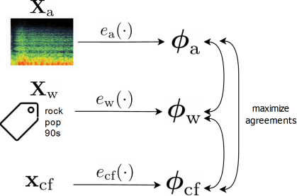
Figure 1: Diagram with architecture of the method

The CF process gets as input a binary matrix, $\mathbf{B}_{\text{cf}}\in\{0,1\}^{M\times M_{\text{pl}}}$, that indicates which songs are included on which playlist, where $M_{\text{pl}}$ is the amount of playlists. Then, we minimize the WARP loss (Weighted Approximate-Rank Pairwise loss) using SGD and the sampling technique defined in ²², to approximate ranks between playlists and songs efficiently. CF outputs the matrices $\mathbf{X}_{\text{cf}}\in\mathbb{R}_{\geq 0}^{M\times F_{\text{cf}}}$ and $\mathbf{Q}_{\text{cf}}\in\mathbb{R}_{\geq 0}^{F_{\text{cf}}\times M_{\text{pl}}}$, where $\mathbf{B}_{\text{cf}}\simeq\mathbf{X}_{\text{cf}}\cdot\mathbf{Q}_{\text{cf}}$. We use each row of $\mathbf{X}_{\text{cf}}$ as the vector $\mathbf{x}_{\text{cf}}^{m}$. We employ $e_{\text{cf}}(\cdot)$ to process the $\mathbf{x}_{\text{cf}}^{m}$, by providing a representation of $\mathbf{x}_{\text{cf}}^{m}$ that is learned specifically for the alignment process that our method tries to achieve. The output of $e_{\text{cf}}(\cdot)$ is the vector $\boldsymbol{\phi}_{\text{cf}}^{m}=e_{\text{cf}}(\mathbf{x}_{\text{cf}}^{m})$, calculated as

$$\boldsymbol{\phi}_{\text{cf}}^{m}=(\text{LN}\circ\text{FF}_{\text{cf2}}\circ\text{DP}\circ\text{ReLU}\circ\text{FF}_{\text{cf1}})(\mathbf{x}_{\text{cf}}^{m})\text{.}$$ (8)

2.2 Optimization and alignment of latent representations

We jointly optimize all encoders using $\mathbb{D}$ and three contrastive losses. We expand previous approaches on audio representation learning using multi-modal alignment, by employing multiple cross-modal and single modal alignment processes. Specifically, we align $\boldsymbol{\phi}_{\text{a}}^{m}$ with $\boldsymbol{\phi}_{\text{w}}^{m}$ (audio-to-genre, A2G, alignment), $\boldsymbol{\phi}_{\text{a}}^{m}$ with $\boldsymbol{\phi}_{\text{cf}}^{m}$ (audio-to-playlist, A2P, alignment), and $\boldsymbol{\phi}_{\text{cf}}^{m}$ with $\boldsymbol{\phi}_{\text{cf}}^{m}$ (genre-to-playlist, G2P, alignment).

We use A2G alignment so that $\boldsymbol{\phi}_{\text{a}}^{m}$ keeps information about musical genre. Additionally, we further enhance the information in $\boldsymbol{\phi}_{\text{a}}^{m}$ by the A2P alignment, which is targeted to allow $\boldsymbol{\phi}_{\text{a}}^{m}$ to have information about playlist associations. Finally, we employ G2P alignment, so that we keep genre and playlist related information tied up together and not let them degenerate to some representation that just helps to minimize the employed losses. Specifically, we use the contrastive loss between two paired examples, $\boldsymbol{\psi}_{\alpha}$ and $\boldsymbol{\psi}_{b}$, defined as ^{14, 17}

$$\mathcal{L}_{\boldsymbol{\psi}_{\alpha},\boldsymbol{\psi}_{b}}=\sum\limits_{i=1}^{M}-\log \frac{\Xi(\boldsymbol{\psi}^{i}_{\alpha},\boldsymbol{\psi}^{i}_{b},\tau)}{\sum\limits_{k=1}^{2M}\mathbbm{1}_{[k\neq i]}\Xi(\boldsymbol{\psi}^{i}_{\alpha},\boldsymbol{\zeta}^{k},\tau)}\text{, where}$$ (9)

$$\Xi(\mathbf{a},\mathbf{b},\tau) =\exp(\text{sim}(\mathbf{a},\mathbf{b})\tau^{-1})\text{,}$$ (10)

$$\text{sim}(\mathbf{a},\mathbf{b}) =\mathbf{a}^{\top}\mathbf{b}(||\mathbf{a}||\;||\mathbf{b}||)^{-1}\text{,}$$ (11)

$$\boldsymbol{\zeta}^{k} =\begin{cases}\boldsymbol{\psi}^{k}_{a}\text{, if }k\leq M\\ \boldsymbol{\psi}^{k-M}_{b}\text{ else}\end{cases}\text{, }$$ (12)

$\mathbbm{1}_{\text{A}}$ is the indicator function with $\mathbbm{1}_{\text{A}}=1$ iff A else 0, and $\tau$ is a temperature hyper-parameter.

We identify $\mathcal{L}_{\text{A2G}}=\mathcal{L}_{\boldsymbol{\phi}_{\text{a}},\boldsymbol{\phi}_{\text{w}}}+\mathcal{L}_{\boldsymbol{\phi}_{\text{w}},\boldsymbol{\phi}_{\text{a}}}$ as the loss for A2G alignment, $\mathcal{L}_{\text{A2P}}=\mathcal{L}_{\boldsymbol{\phi}_{\text{a}},\boldsymbol{\phi}_{\text{cf}}}+\mathcal{L}_{\boldsymbol{\phi}_{\text{cf}},\boldsymbol{\phi}_{\text{a}}}$ as the loss for A2P alignment, and $\mathcal{L}_{\text{G2P}}=\mathcal{L}_{\boldsymbol{\phi}_{\text{w}},\boldsymbol{\phi}_{\text{cf}}}+\mathcal{L}_{\boldsymbol{\phi}_{\text{cf}},\boldsymbol{\phi}_{\text{w}}}$ as the loss for G2P alignment. We optimize all of our encoders, obtaining $e_{\text{a}}^{\star}$, by minimizing the

$$\mathcal{L}_{\text{tot}}=\lambda_{\text{A2G}}\mathcal{L}_{\text{A2G}}+\lambda_{\text{A2P}}\mathcal{L}_{\text{A2P}}+\lambda_{\text{G2P}}\mathcal{L}_{\text{G2P}}\text{,}$$ (13)

where $\lambda_{\cdot}$ are different hyper-parameters used as weighting factors for the losses.

3 Evaluation

To evaluate our method, we employ Melon Playlist Dataset ²³ as $\mathbb{D}$, in order to obtain $e_{\text{a}}$. Then, we assess the learned representations by $e_{\text{a}}$ applying it in different downstream tasks. Specifically, we focus on genre classification, audio-tagging, and automatic playlist continuation. For each of the tasks, we employ $e_{\text{a}}$ as audio encoder, which will provide embeddings to a classifier, trained for the corresponding task.

We assess the benefit of the contribution of each of the encoders of our method, by comparing our method using three encoders ($\text{Contr}_{\text{CF-G}}$) with our method but using only $e_{\text{a}}$ and $e_{\text{w}}$ ($\text{Contr}_{\text{G}}$), and using only $e_{\text{a}}$ and $e_{\text{cf}}$ ($\text{Contr}_{\text{CF}}$). In addition, we compare the performance on each task using a baseline architecture that directly predicts the target information from the audio encoder. We refer to these methods as $\text{B-line}_{\text{G}}$ for the model trained with genre information, $\text{B-line}_{\text{CF}}$ for the model trained to predict CF information and $\text{B-line}_{\text{CF-G}}$ for the model trained to predict both types of information at the same time.

3.1 Melon Playlist Dataset and audio features

The dataset $\mathbb{D}$ used to train the models was originally collected Melon, a Korean music streaming service. The dataset consists of $M$=649,091 songs, represented by their mel-spectrograms, and $M_{\text{pl}}$=148,826 playlists. The number of unique genres asociated with the songs is 219. In order to train the model we split the songs of the dataset in train (80%), validation (10%) and test (10%). The split was done applying a stratified approach ²⁴ in order to assure a similar distribution of example in all the sets for the genres associated to the songs.

The pre-computed mel-spectrograms provided in the dataset correspond to a range of 20 to 50 seconds with a resolution of $F_{\text{a}}=48$ mel-bands. Such reduced mel-bands resolution did not negatively affect the performance of the auto-tagging approaches in our previous study ²⁵ and have a significantly lower quality of reconstructed audio which allows to avoid copyright issues. Following the previous work ²⁶, we randomly select sections the songs to train the audio encoder, using $T_{\text{a}}=256$.

3.2 Parameters optimization

Following the best performance in previous work ^{1, 26} the audio encoder use $Z$=7 layers and $K$=3. We conducted a preliminary evaluation to select the hyper-parameters of the models, comparing the loss in the validation and training set to prevent the models of overfitting. We defined the dimensions for CF representations to $F_{\text{cf}}$= 300 and genres representations $F_{\text{w}}$= 200 with $T_{\text{w}}<=$ 10 genres per song. From the same preliminary evaluation we defined the temperature $\tau$=0.1, batch size of 128, learning rate of 1e-4, dropout of 0.5 and the number of heads for self-attention of 4. We did not experiment with changing the weights $\lambda$ for the different losses and we used $\lambda_{\text{A2G}}=\lambda_{\text{A2P}}=\lambda_{\text{G2P}}=1$.

3.3 Downstream tasks

Once the models are trained with the Melon Playlist Dataset, we use the pre-trained models to generate an embedding from the audio of each song in the different datasets. Then, we use the generated embeddings and compare the performance for each particular task. In the following, we describe each downstream task and the dataset used.

Genre Classification We use the fault-filtered version of the GTZAN dataset ^{27, 28} consisting of music excepts of 30 seconds, single-labeled using 10 classes and split in pre-computed sets of 443 songs for training and 290 for testing. We train a multilayer perceptron (MLP) of one hidden layer of size 256 with ReLU activations, using the training set and compute its accuracy on the test set. In order to obtain an unbiased evaluation, we repeat this process 10 times and average the accuracies. We consider each embedding frame of a track as a different training instance, and when inferring the genres, we apply a majority voting strategy. We also include the performance of pre-trained embedding models taken from the literature ^{29, 30, 31}, using the results reported in ³⁰.

Automatic Tagging. We rely on the MTG-Jamendo dataset ³² which contains over 55,000 full audio tracks multi-labeled using 195 different tags from genre, instrument, and mood/theme categories. For this task, we train a MLP that takes our pre-trained audio embeddings as input. We compute the embedding of all the tracks by averaging their embeddings computed on non-overlapping frames with the mean statistic. The model is composed of two hidden layers of size 128 and 64 with ReLU activations, it includes batch normalizations after each layer and a dropout regularization after the penultimate layer. We use the validation sets for early stopping and we finally evaluate the performances on the test sets using ROC AUC. These evaluations are done on the three separated category of tags, each of them uses its own split. We repeat the procedures 10 times and report the mean average.

Playlist Continuation. We make use of the playlists from the Melon Playlist Dataset that contain at least one track in our test set (not used when training our embedding model). This provides 104,410 playlists, for the which we aim at providing 100 continuation tracks. We compute the embedding of all the tracks by averaging their embeddings computed on non-overlapping frames with the mean statistic. Then, for each track in a playlist, we compute the 100 most similar tracks, among the ones from the test set. These tracks are obtained using the cosine similarity in the embedding space. Among all the retrieved similar tracks for a playlist, we finally select the 100 most repeated ones. We compare these to the ground truth using normalized Discounted Cumulative Gain (nDCG) and Mean Average Precision (MAP) ³⁴, which are commonly used to evaluate the performance of music recommendation systems. These ranking metrics evaluate the order of the items for each playlist returned by the prediction. They return a higher score for a given playlist if the predicted ranked list contains items in the test set closer to the top.

4 Results

Table 1: GTZAN results

Model	Mean Accuracy $\pm$ STD
$\text{B-line}_{\text{G}}$	63.28 $\pm$ 1.19
$\text{B-line}_{\text{CF}}$	57.12 $\pm$ 1.82
$\text{B-line}_{\text{CF-G}}$	64.35 $\pm$ 1.10
$\text{Contr}_{\text{G}}$	76.78 $\pm$ 1.22
$\text{Contr}_{\text{CF}}$	67.12 $\pm$ 0.94
$\text{Contr}_{\text{CF-G}}$	75.29 $\pm$ 1.32
VGGish Audioset 31	77.58
OpenL3 Audioset 29	74.65
musicnn MSD 30	77.24

Focusing on genre classification, the results in Table 1 show that the performance of the audio embedding when trained using the contrastive loss is always higher than using the models trained directly to predict the modality information (B-line). The best performance is obtained with $\text{Contr}_{\text{G}}$ with a similar result to when also considering CF information when training the embedding model ($\text{Contr}_{\text{CF-G}}$). We also see that the performances of the $\text{Contr}_{\text{G}}$ model are comparable with state-of-the-art pre-trained embeddings (VGGish audioset) ^{31, 30}. This is particularly interesting since a large percentage of the Melon Playlist Dataset consists of korean music, which can be different from popular western music from the GTZAN collection.

Table 2: Automatic tagging results

	ROC AUC $\pm$ STD
Model	Genre	Mood	Instrument
$\text{B-line}_{\text{G}}$	0.840 $\pm$ 0.004	0.722 $\pm$ 0.004	0.781 $\pm$ 0.005
$\text{B-line}_{\text{CF}}$	0.836 $\pm$ 0.002	0.722 $\pm$ 0.003	0.770 $\pm$ 0.008
$\text{B-line}_{\text{CF-G}}$	0.845 $\pm$ 0.004	0.727 $\pm$ 0.006	0.785 $\pm$ 0.004
$\text{Contr}_{\text{G}}$	0.847 $\pm$ 0.004	0.732 $\pm$ 0.005	0.797 $\pm$ 0.005
$\text{Contr}_{\text{CF}}$	0.845 $\pm$ 0.004	0.732 $\pm$ 0.004	0.793 $\pm$ 0.007
$\text{Contr}_{\text{CF-G}}$	0.843 $\pm$ 0.004	0.733 $\pm$ 0.005	0.791 $\pm$ 0.006

Automatic Tagging. From the results in Table 2 we see that the methods based on contrastive learning outperform the baselines in almost all the cases. The best results for the instrument and genre tags is obtained with the $\text{Contr}_{\text{G}}$ model. For the mood tags the best performance is achieved with $\text{Contr}_{\text{CF-G}}$, which takes advantage of the information in the playlists and the genre annotations.

Table 3: Playlist generation results

Model	NDCG@100	MAP@100
random	0.0005	0.0001
$\text{B-line}_{\text{G}}$	0.0044	0.0007
$\text{B-line}_{\text{CF}}$	0.0035	0.0007
$\text{B-line}_{\text{CF-G}}$	0.0042	0.0008
$\text{Contr}_{\text{G}}$	0.0074	0.0016
$\text{Contr}_{\text{CF}}$	0.0076	0.0017
$\text{Contr}_{\text{CF-G}}$	0.0085	0.0020

The results for the task of Automatic playlist continuation follow the same trend of the other tasks. The models trained using the contrastive loss perform better than the baselines trained directly to predict the genres or the CF representation. The best performance is obtained with the $\text{Contr}_{\text{CF-G}}$ model, which combines genre and CF information.

5 Conclusions

In this work, we propose a method for learning an audio representation, by combining multiple sources of information related to the music using contrastive learning. We evaluate the method by pre-traing the model using information from the Melon Playlist Dataset and we compare the performance in three downstream tasks in the music domain (genre classification, automatic tagging, and automatic playlist continuation). We see that using contrastive learning allows us to reach higher performance than using the models trained directly to predict the genre or the collaborative filtering information. This indicates that contrastive learning is effective at learning simultaneously from heterogeneous information, enabling us to improve the overall performance across different tasks.

The dataset used for training our embedding model offers additional types of information that we did not use. They include title, playlist tags and authors, as well as other metadata of the tracks. As future work, we propose incorporating this playlist-level information which will require an additional level of abstraction to our architecture.

References

- 1 M. Won, S. Oramas, O. Nieto, F. Gouyon, and X. Serra, “Multimodal metric learning for tag-based music retrieval,” arXiv preprint arXiv:2010.16030, 2020.
- 2 Ò. Celma and P. Herrera, “A new approach to evaluating novel recommendations,” in Proceedings of the 2008 ACM conference on Recommender systems, 2008, pp. 179–186.
- 3 F. Korzeniowski, O. Nieto, M. McCallum, M. Won, S. Oramas, and E. Schmidt, “Mood classification using listening data,” arXiv preprint arXiv:2010.11512, 2020.
- 4 S. Oramas, F. Barbieri, O. Nieto, and X. Serra, “Multimodal deep learning for music genre classification,” Transactions of the International Society for Music Information Retrieval. 2018; 1 (1): 4-21., 2018.
- 5 D. Surís, A. Duarte, A. Salvador, J. Torres, and X. Giró-i Nieto, “Cross-modal embeddings for video and audio retrieval,” in Proceedings of the European conference on computer vision (ECCV), 2018, pp. 0–0.
- 6 A. Radford, L. Metz, and S. Chintala, “Unsupervised representation learning with deep convolutional generative adversarial networks,” arXiv preprint arXiv:1511.06434, 2015.
- 7 P. Alonso-Jiménez, D. Bogdanov, J. Pons, and X. Serra, “Tensorflow audio models in essentia,” in 2020 IEEE International Conference on Acoustics, Speech and Signal Processing (ICASSP), 2020, pp. 266–270.
- 8 A. Zhai and H.-Y. Wu, “Classification is a strong baseline for deep metric learning,” arXiv preprint arXiv:1811.12649, 2018.
- 9 J. Lee, N. J. Bryan, J. Salamon, Z. Jin, and J. Nam, “Metric learning vs classification for disentangled music representation learning,” in Proc. of the 21st International Society for Music Information Retrieval Conference (ISMIR), 2020.
- 10 P. H. Le-Khac, G. Healy, and A. F. Smeaton, “Contrastive representation learning: A framework and review,” IEEE Access, 2020.
- 11 K. Q. Weinberger and L. K. Saul, “Distance metric learning for large margin nearest neighbor classification.” Journal of Machine Learning Research, vol. 10, no. 2, 2009.
- 12 J. Choi, J. Lee, J. Park, and J. Nam, “Zero-shot learning for audio-based music classification and tagging,” arXiv preprint arXiv:1907.02670, 2019.
- 13 A. v. d. Oord, Y. Li, and O. Vinyals, “Representation learning with contrastive predictive coding,” arXiv preprint arXiv:1807.03748, 2018.
- 14 T. Chen, S. Kornblith, M. Norouzi, and G. Hinton, “A simple framework for contrastive learning of visual representations,” arXiv preprint arXiv:2002.05709, 2020.
- 15 E. Fonseca, D. Ortego, K. McGuinness, N. E. O’Connor, and X. Serra, “Unsupervised contrastive learning of sound event representations,” arXiv preprint arXiv:2011.07616, 2020.
- 16 A. Saeed, D. Grangier, and N. Zeghidour, “Contrastive learning of general-purpose audio representations,” arXiv preprint arXiv:2010.10915, 2020.
- 17 X. Favory, K. Drossos, T. Virtanen, and X. Serra, “Coala: Co-aligned autoencoders for learning semantically enriched audio representations,” in International Conference on Machine Learning (ICML), Workshop on Self-supervised learning in Audio and Speech, 2020.
- 18 P. Khosla, P. Teterwak, C. Wang, A. Sarna, Y. Tian, P. Isola, A. Maschinot, C. Liu, and D. Krishnan, “Supervised contrastive learning,” arXiv preprint arXiv:2004.11362, 2020.
- 19 X. Favory, K. Drossos, T. Virtanen, and X. Serra, “Learning contextual tag embeddings for cross-modal alignment of audio and tags,” arXiv preprint arXiv:2010.14171, 2020.
- 20 A. Vaswani, N. Shazeer, N. Parmar, J. Uszkoreit, L. Jones, A. N. Gomez, Ł. Kaiser, and I. Polosukhin, “Attention is all you need,” Advances in neural information processing systems, vol. 30, pp. 5998–6008, 2017.
- 21 T. Mikolov, K. Chen, G. S. Corrado, and J. Dean, “Efficient estimation of word representations in vector space,” in International Conference of Learning Representations (ICLR), 2013.
- 22 J. Weston, S. Bengio, and N. Usunier, “Wsabie: Scaling up to large vocabulary image annotation,” 2011.
- 23 A. Ferraro, Y. Kim, S. Lee, B. Kim, N. Jo, S. Lim, S. Lim, J. Jang, S. Kim, X. Serra, and D. Bogdanov, “Melon playlist dataset: a public dataset for audio-based playlist generation and music tagging,” in International Conference on Acoustics, Speech and Signal Processing (ICASSP 2021), 2021.
- 24 K. Sechidis, G. Tsoumakas, and I. Vlahavas, “On the stratification of multi-label data,” in Joint European Conference on Machine Learning and Knowledge Discovery in Databases. Springer, 2011, pp. 145–158.
- 25 A. Ferraro, D. Bogdanov, X. S. Jay, H. Jeon, and J. Yoon, “How low can you go? Reducing frequency and time resolution in current CNN architectures for music auto-tagging,” in 2020 28th European Signal Processing Conference (EUSIPCO). IEEE, pp. 131–135.
- 26 M. Won, A. Ferraro, D. Bogdanov, and X. Serra, “Evaluation of CNN-based automatic music tagging models,” in Proceedings of the SMC2020 - 17th Sound and Music Computing Conference, 2020.
- 27 G. Tzanetakis and P. Cook, “Musical genre classification of audio signals,” IEEE Transactions on speech and audio processing, vol. 10, no. 5, pp. 293–302, 2002.
- 28 C. Kereliuk, B. L. Sturm, and J. Larsen, “Deep learning and music adversaries,” IEEE Transactions on Multimedia, vol. 17, no. 11, pp. 2059–2071, 2015.
- 29 J. Cramer, H.-H. Wu, J. Salamon, and J. P. Bello, “Look, listen, and learn more: Design choices for deep audio embeddings,” in ICASSP 2019-2019 IEEE International Conference on Acoustics, Speech and Signal Processing (ICASSP). IEEE, 2019, pp. 3852–3856.
- 30 J. Pons and X. Serra, “Musicnn: pre-trained convolutional neural networks for music audio tagging,” in Late-breaking/demo session in 20th International Society for Music Information Retrieval Conference (LBD-ISMIR2019), 2019.
- 31 J. F. Gemmeke, D. P. Ellis, D. Freedman, A. Jansen, W. Lawrence, R. C. Moore, M. Plakal, and M. Ritter, “Audio set: An ontology and human-labeled dataset for audio events,” in 2017 IEEE International Conference on Acoustics, Speech and Signal Processing (ICASSP). IEEE, 2017, pp. 776–780.
- 32 D. Bogdanov, M. Won, P. Tovstogan, A. Porter, and X. Serra, “The MTG-Jamendo dataset for automatic music tagging,” in Proceedings of the Machine Learning for Music Discovery Workshop, 36th International Conference on Machine Learning, ML4MD at ICML 2019, 2019.
- 33 S. Dasgupta and Y. Freund, “Random projection trees and low dimensional manifolds,” in Proceedings of the fortieth annual ACM symposium on Theory of computing, 2008, pp. 537–546.
- 34 F. Ricci, L. Rokach, B. Shapira, and P. B. Kantor, Recommender Systems Handbook, 1st ed. Berlin, Heidelberg: Springer-Verlag, 2010.