$L_{1}$ and $L_{\infty}$ stability of transition densities of perturbed diffusions††The study has been funded by the Russian Science Foundation (project β„–Β 20-11-20119)

I.Bitter, V. Konakov Laboratory of Stochastic Analysis, HSE University, Pokrovsky Blvd, 11, Moscow, Russian Federation. ilya.bitter@yandex.ruLaboratory of Stochastic Analysis, HSE University, Pokrovsky Blvd, 11, Moscow, Russian Federation. vkonakov@hse.ru
Abstract

In this paper, we derive a stability result for $L_{1}$ and $L_{\infty}$ perturbations of diffusions under weak regularity conditions on the coefficients. In particular, in contrast to [17, 18], the drift terms we consider can be unbounded with at most linear growth, and we do not require uniform convergence of perturbed diffusions. Instead, we require a weaker convergence condition in a special metric introduced in this paper, related to the Holder norm of the diffusion matrix differences. Our approach is based on a special version of the McKean-Singer parametrix expansion.

Keywords: unbounded drift, density, perturbed diffusion, stability, parametrix.

MSC 2020: Primary: 60H10, 60H30; Secondary: 35K10.

1 Introduction

1.1 Setting

For a fixed deterministic horizon $T>0,$ let us consider the following $d$ - dimensional, non-degenerate Ito’s diffusion

$$dX_{t}=b\left(t,X_{t}\right)dt+\sigma\left(t,X_{t}\right)dW_{t},\quad t\in[0,T].$$ (1.1)

$W_{t}$ stands for a $d$ - dimensional Brownian motion on some filtered complete probability space $(\Omega,\mathcal{F},(\mathcal{F}_{t})_{t\geq 0},\mathbb{P})$ satisfying the usual conditions, and the coefficients are assumed to be measurable, rough in time, and HΓΆlder in space, with potentially unbonded drift. Also $a(t,x):=\sigma\sigma^{*}(t,x)$ is assumed to be uniformly elliptic. The infinitesimal generator of (1.1) at time $u$ and for all $\varphi\in C_{0}^{2}\left(\mathbb{R}^{d},\mathbb{R}\right),z\in\mathbb{R}^{d}$, is defined as follows:

$\displaystyle L_{u}\varphi(z)=\frac{1}{2}\operatorname{Tr}\left(\sigma\sigma^{*}(u,z)D_{z}^{2}\varphi(z)\right)+\left\langle b(u,z),D_{z}\varphi(z)\right\rangle=$ (1.2)
$\displaystyle=\frac{1}{2}\sum_{i,j=1}^{d}a_{ij}(u,z)\frac{\partial^{2}{\varphi}(u,z)}{\partial z_{i}\partial z_{j}}+\sum_{i=1}^{d}b_{i}(u,z)\frac{\partial{\varphi}(u,z)}{\partial z_{i}}.$ (1.3)

We now introduce, for a given parameter $\varepsilon>0,$ a perturbed version of (1.1) with dynamics

$$dX_{t}^{\varepsilon}=b_{\varepsilon}\left(t,X_{t}^{\varepsilon}\right)dt+\sigma_{\varepsilon}\left(t,X_{t}^{\varepsilon}\right)dW_{t},\quad t\in[0,T],$$ (1.4)

where the coefficients $b_{\varepsilon},\sigma_{\varepsilon}$ satisfy at least the same assumptions as $b,\sigma$ and are in some sense meant to be close to $b,\sigma$ when $\varepsilon$ is small. When both coefficients $b,\sigma$ are bounded and Holder continuous, it is well known that there exists a unique weak solution to (1.1), which has a density [14, 15, 17]. Moreover, combining the parametrix method to get the upper bound [17, 11], and the chaining method to obtain the lower bound [4], it can be shown [2, 3] that the transition density $p(0,x,t,y)$ satisfies the two sided Gaussian bounds

$$C^{-1}g_{\lambda^{-1}}(t,x-y)\leq p(0,x,t,y)\leq Cg_{\lambda}(t,x-y),$$

where

$$g_{\lambda}(t,x)=t^{-d/2}\exp\left(-\frac{\lambda|x|^{2}}{t}\right),\lambda\in(0,1],\quad t>0.$$

Such methods were successfully developed for more general cases, namely, for operators satisfying strong HΓΆrmander conditions and Kolmogorov operators with linear drifts [16, 21, 13]. When the drift is unbounded and non-linear, fewer results are available. To obtain an upper bound, we need to control the terms of the parametrix series, and in the case of unbounded drift it becomes a delicate problem. For the drifts with sublinear growth, namely, $|b(t,x)|\leq C\left(|x|^{\beta}+1\right),\beta\in(0,1),$ the generalization of the parametrix method was obtained in [11], but the method developed there fails for the drifts with linear growth. It seems quite plausible that a linearly growing drift is exactly the boundary case, starting from which, it is necessary to introduce a forward flow corresponding to the transport of the initial condition or, equivalently, a backward flow corresponding to the transport of the terminal condition [20, 12, 16]. For unbounded at most linearly growing drift, the upper bound for the transition density may be obtained by using the truncation method introduced in [12], see also [20]. This method consists in viewing a Fleming logarithmic transformation (see [12, 22]) of a transition density as a value function of a certain stochastic control problem [10], the desired density estimates are obtained by choosing appropriate controls. In the case of unbounded drift, the truncation method allows one to obtain an upper bound for a transition density, but, in order to study the sensitivity of transition densities w.r.t. the perturbations of coefficients one needs to work with a complete parametrix series without truncation.

Note also that the upper bounds for the total variation, entropy and Kantorovich distances between two solutions to Fokker-Planck-Kolmogorov equations with different diffusion matrices and drifts on $\mathbb{R}^{d}\times[0,T]$ with fixed $T>0$ were obtained in [7], and upper bounds for the distances between stationary solutions to Fokker-Planck-Kolmogorov equations with different diffusion matrices and drifts were obtained in [8].

The aim of the present paper is to extend the stability results [17] to the case of nonlinear unbounded drift with at most linear growth. Moreover, we replace the condition of $L_{\infty}$ - closeness by the weaker one, namely, by $L_{1}$ - closeness. To this end, the complete parametrix series will be constructed, which, in contrast to [11], will be convergent also for drifts with linear growth.

Diffusions with the dynamics (1.1) and unbounded drifts appear in many applied problems. Important applications can, for instance, be found in mathematical finance. It is often very useful to know how a perturbation of the volatility $\sigma$ impacts the density, and therefore the associated option prices [9, 6]. In the framework of parameter estimation, it can be useful, having at the hand estimators $\left(b_{\varepsilon},\sigma_{\varepsilon}\right)$ of the true parameters $\left(b,\sigma\right)$ and some controls for the differences $\left|b-b_{\varepsilon}\right|,\left|\sigma-\sigma_{\varepsilon}\right|$ in a suitable sense, to quantify the difference $p-p_{\varepsilon}$ of the densities corresponding, respectively, to the dynamics with the estimated parameters and the one of the model. Another important application includes the case of mollification by spatial convolution. This specific kind of perturbation is useful for investigating the error between the densities of a non-degenerate diffusion of type (1.1) with HΓΆlder coefficients (or with piecewise smooth bounded drift) and its Euler scheme. In this framework, some explicit convergence results can be found in [18] and for measurable bounded drift in [5]. In summary, stability results can be useful in every applied field where the diffusion coefficients might be misspecified.


This paper is organized as follows. In the next subsection, we introduce our assumptions and state the main result. Section 2 contains an introduction to some crucial facts about parametrix expansion and deterministic flow associated with a drift of corresponding diffusion. In Section 3, we derive our main results in $L_{1}$ and $L_{\infty}$ cases, respectively. Additional proofs of technical lemmas are given in Appendix. In what follows, the letter $C$ stands for a positive constant, only depending on the quantities in the assumptions; in the context of the proofs, it’s value may vary from line to line.

1.2 Assumptions and Main Result

In this paper, we study the difference between transition densities of the process (1.1) and its perturbed version (1.4). A similar problem for processes with bounded drift was discussed in [17]. In contrast, we consider a more general class of processes with growing drift. In our setting, we prove that the difference between $p$ and $p_{\varepsilon}$ admits an upper bound in terms of $L_{1}-L_{1}$ norm: for probability measure $\mu$, we denote

$$||f(x,y)||_{L_{1}^{\mu}\left(\mathbb{R}^{d},L_{1}(\mathbb{R}^{d})\right)}=\int_{\mathbb{R}^{d}}\int_{\mathbb{R}^{d}}|f(x,y)|dy\ \mu(dx).$$

For any Borel sets $A\in\mathcal{B}([t,s]),\ B\in\mathcal{B}(\mathbb{R}^{d})$ and $x\in\mathbb{R}^{d}$, define the probability measures

$$\beta(A)=\int_{A}\mathfrak{B}\left(u;1,\frac{\gamma}{2}\right)du,\ \bar{\lambda}(B)=\int_{B}\bar{p}(t,s,x,y)dy,$$

and $L_{1}$-space of functions defined on $\left([t,s]\times\mathbb{R}^{d}\times\mathbb{R}^{d},\beta\times\bar{\lambda}\times\mu\right)$

$$||f(u,x,y)||_{L_{1}}=\left[\int_{\mathbb{R}^{d}}\int_{R^{d}}\int_{t}^{s}\mathfrak{B}(u;1,\dfrac{\gamma}{2})\left|f(u,x,y)\right|\bar{p}(t,s,x,y)\ du\ dy\ \mu(dx)\right].$$ (1.5)

Here $\mathfrak{B}(u;1,\dfrac{\gamma}{2})$ is a beta-density on the interval $[t,s]$, $0\leq t<s\leq T$, and $\bar{p}(t,s,x,y)$ is the transition density of some an auxiliary diffusion process that will be introduced in (2.18). Recall that

$$\mathfrak{B}(u;\alpha,\beta)=\dfrac{1}{B(\alpha,\beta)}(u-t)^{\alpha-1}(s-u)^{\beta-1}(s-t)^{1-\alpha-\beta},\ u\in[t,s],$$

where $B(\alpha,\beta)$ is the Beta-function. It is natural in this case to consider the perturbation in $L_{1}$ sense and to use the beta-density as a weight function in the time variable. This choice is well-adapted to the beta function appearing in the upper bounds for the parametrix series terms.

Let us introduce the following assumptions. Below, the parameter $\varepsilon>0$ is fixed and the constants appearing in the assumptions do not depend on it. In what follows, it is important that we consider the problem globally, namely on the product space $[0,T]\times\mathbb{R}^{d}$.

  • (A1)

    (Uniform Ellipticity.) Matrices $a=\sigma\sigma^{*}$ and $a_{\varepsilon}=\sigma_{\varepsilon}\sigma^{*}_{\varepsilon}$ are uniformly elliptic, i.e., there exists a positive constant $\Lambda\geq 1,$ such that $\forall(t,x)\in[0,T]\times\mathbb{R}^{d}$,

    $\displaystyle\Lambda^{-1}|w|^{2}\leq\langle a(t,x)w,w\rangle\leq\Lambda|w|^{2},\quad\forall w\in\mathbb{R}^{d}.$ (1.6)
    $\displaystyle\Lambda^{-1}|w|^{2}\leq\langle a_{\varepsilon}(t,x)w,w\rangle\leq\Lambda|w|^{2},\quad\forall w\in\mathbb{R}^{d}.$ (1.7)

    This condition also implies the uniform ellipticity of matrices $a^{-1}$ and $a^{-1}_{\varepsilon}$.

  • (A2)

    (Regularity.) The diffusion coefficients and the drifts of (1.1) and (1.4) are HΓΆlder and Lipschitz continuous in space, respectively: for $\gamma\in(0,1],K>0\ \text{and}\ \forall(t,x),(s,y)\in[0,T]\times\mathbb{R}^{d}$,

    $$\left|\sigma(t,x)-\sigma(t,y)\right|+\left|\sigma_{\varepsilon}(t,x)-\sigma_{\varepsilon}(t,y)\right|\leq K\left|x-y\right|^{\gamma},$$ (1.8)
    $$\left|b(t,x)-b(t,y)\right|+\left|b_{\varepsilon}(t,x)-b_{\varepsilon}(t,y)\right|\leq K\left|x-y\right|,$$ (1.9)
    $$\left|b(t,\textbf{0})\right|+\left|b_{\varepsilon}(t,\textbf{0})\right|\leq K,\ \textbf{0}\in\mathbb{R}^{d}.$$ (1.10)

    Clearly, if $\sigma(t,\cdot)$ is bounded and HΓΆlder continuous so is $a(t,\cdot)$. Also, the regularity conditions imply at most linear growth of the drift coefficients:

    $\displaystyle|b(t,x)|+|b_{\varepsilon}(t,x)|\leq K\left(1+|x|\right)\quad\forall(t,x)\in[0,T]\times\mathbb{R}^{d}.$ (1.11)

    Thanks to the Lipschitz continuity and at most linear growth of the drift term in (1.1), the following Cauchy problem has a unique solution for fixed $(s,y)\in[0,T]\times\mathbb{R}^{d}$, defined globally on $[0,s]$:

    ΞΈΛ™w,s​(y)=b​(w,ΞΈw,s​(y)),ΞΈs,s​(y)=y.formulae-sequencesubscriptΛ™πœƒπ‘€π‘ π‘¦π‘π‘€subscriptπœƒπ‘€π‘ π‘¦subscriptπœƒπ‘ π‘ π‘¦π‘¦\dot{\theta}_{w,s}(y)=b(w,\theta_{w,s}(y)),\quad\theta_{s,s}(y)=y. (1.13)

    Throughout the paper, we will call the deterministic flow solving ODE (1.13) the flow associated with drift $b$. In the same way, ΞΈw,sΡ​(y)subscriptsuperscriptπœƒπœ€π‘€π‘ π‘¦\theta^{\varepsilon}_{w,s}(y) is the flow associated with $b_{\varepsilon}$.

  • (A3)

    (Almost equivalence of the flows.)

    There exists a positive constant $C_{\theta}$ such that $\forall 0\leq t<s\leq T$, uniformly in space,

    ∫ts|bΡ​(u,x)βˆ’b​(u,x)|​𝑑u≀Cθ​sβˆ’t.superscriptsubscript𝑑𝑠subscriptπ‘πœ€π‘’π‘₯𝑏𝑒π‘₯differential-d𝑒subscriptπΆπœƒπ‘ π‘‘\int_{t}^{s}\left|b_{\varepsilon}(u,x)-b(u,x)\right|du\leq C_{\theta}\sqrt{s-t}. (1.14)

    As a consequence, the flows ΞΈw,s​(y)subscriptπœƒπ‘€π‘ π‘¦\theta_{w,s}(y) and ΞΈw,sΡ​(y)subscriptsuperscriptπœƒπœ€π‘€π‘ π‘¦\theta^{\varepsilon}_{w,s}(y) associated with the drifts of (1.1) and (1.4) are almost equivalent:

    |ΞΈt,sΡ​(y)βˆ’ΞΈt,s​(y)|=|∫tsbΡ​(u,ΞΈu,sΡ​(y))βˆ’b​(u,ΞΈu,s​(y))​d​u|≀subscriptsuperscriptπœƒπœ€π‘‘π‘ π‘¦subscriptπœƒπ‘‘π‘ π‘¦superscriptsubscript𝑑𝑠subscriptπ‘πœ€π‘’subscriptsuperscriptπœƒπœ€π‘’π‘ π‘¦π‘π‘’subscriptπœƒπ‘’π‘ π‘¦π‘‘π‘’absent\displaystyle\left|\theta^{\varepsilon}_{t,s}(y)-\theta_{t,s}(y)\right|=\left|\int_{t}^{s}b_{\varepsilon}\left(u,\theta^{\varepsilon}_{u,s}(y)\right)-b\left(u,\theta_{u,s}(y)\right)du\right|\leq (1.15)
    ≀Kβ€‹βˆ«ts|ΞΈu,sΡ​(y)βˆ’ΞΈu,s​(y)|​𝑑u+∫ts|bΡ​(u,ΞΈu,s​(y))βˆ’b​(u,ΞΈu,s​(y))|​𝑑u≀Cθ​sβˆ’tabsent𝐾superscriptsubscript𝑑𝑠subscriptsuperscriptπœƒπœ€π‘’π‘ π‘¦subscriptπœƒπ‘’π‘ π‘¦differential-d𝑒superscriptsubscript𝑑𝑠subscriptπ‘πœ€π‘’subscriptπœƒπ‘’π‘ π‘¦π‘π‘’subscriptπœƒπ‘’π‘ π‘¦differential-d𝑒subscriptπΆπœƒπ‘ π‘‘\displaystyle\leq K\int_{t}^{s}\left|\theta^{\varepsilon}_{u,s}(y)-\theta_{u,s}(y)\right|du+\int_{t}^{s}\left|b_{\varepsilon}\left(u,\theta_{u,s}(y)\right)-b\left(u,\theta_{u,s}(y)\right)\right|du\leq C_{\theta}\sqrt{s-t} (1.16)

    by the GrΓΆnwall inequality.


    For a given $\varepsilon>0$, we say that the assumption (A) holds when conditions (A1) - (A3) are in force. Let us now introduce, under (A), the quantities that will bound the difference of the densities $p$ and $p_{\varepsilon}$ in our main result below. Set for $\varepsilon>0$:

    ΔΡ,b​(t,s)=βˆ₯|(bβˆ’bΞ΅)​(u,ΞΈu,s​(y))|1βˆ₯L1,subscriptΞ”πœ€π‘π‘‘π‘ subscriptdelimited-βˆ₯βˆ₯subscript𝑏subscriptπ‘πœ€π‘’subscriptπœƒπ‘’π‘ π‘¦1subscript𝐿1\displaystyle\Delta_{\varepsilon,b}(t,s)=\big{\lVert}\left|\left(b-b_{\varepsilon}\right)(u,\theta_{u,s}(y))\right|_{1}\big{\rVert}_{L_{1}}, (1.17)
    ΔΡ,σ​(t,s)=βˆ₯|(Οƒβˆ’ΟƒΞ΅)​(u,ΞΈu,s​(y))|Ξ³βˆ₯L1,subscriptΞ”πœ€πœŽπ‘‘π‘ subscriptdelimited-βˆ₯βˆ₯subscript𝜎subscriptπœŽπœ€π‘’subscriptπœƒπ‘’π‘ π‘¦π›Ύsubscript𝐿1\displaystyle\Delta_{\varepsilon,\sigma}(t,s)=\big{\lVert}\left|\left(\sigma-\sigma_{\varepsilon}\right)(u,\theta_{u,s}(y))\right|_{\gamma}\big{\rVert}_{L_{1}}, (1.18)
    $$\displaystyle\Delta_{\varepsilon}:=\Delta_{\varepsilon,b}+\Delta_{\varepsilon,\sigma}.$$ (1.19)

    Here $|\cdot|_{\beta}$ stands for the expression consisting of two terms:

    |f​(t,x)|Ξ²:=|f​(t,x)|+supyβˆˆβ„d,yβ‰ x|f​(t,x)βˆ’f​(t,y)||xβˆ’y|Ξ².assignsubscript𝑓𝑑π‘₯𝛽𝑓𝑑π‘₯subscriptsupremumformulae-sequence𝑦superscriptℝ𝑑𝑦π‘₯𝑓𝑑π‘₯𝑓𝑑𝑦superscriptπ‘₯𝑦𝛽|f(t,x)|_{\beta}:=|f(t,x)|+\sup_{y\in\mathbb{R}^{d},y\neq x}\frac{|f(t,x)-f(t,y)|}{|x-y|^{\beta}}.

Now, for an arbitrary positive constant $\delta\in(\gamma/2,\gamma)$ and parameter $\alpha>0$, we consider diagonal and off-diagonal maxima:

$$M_{\varepsilon,\alpha,\delta}=\max\limits_{\left(s-t\right)\leq\alpha}(s-t)^{\delta-\gamma/2}\left(\Delta_{\varepsilon}(t,s)\right)^{\gamma-\delta},$$
$$\bar{M}_{\varepsilon,\alpha,\delta}=\max\limits_{\left(s-t\right)\leq\alpha}\left(\Delta_{\varepsilon}(t,s)\right)^{\gamma-\delta},$$
$$M^{\mathcal{C}}_{\varepsilon,\alpha,\delta}=\max\limits_{\left(s-t\right)>\alpha}(s-t)^{\delta-\gamma/2}\left(\Delta_{\varepsilon}(t,s)\right)^{\gamma-\delta},$$
$$\bar{M}^{\mathcal{C}}_{\varepsilon,\alpha,\delta}=\max\limits_{\left(s-t\right)>\alpha}\left(\Delta_{\varepsilon}(t,s)\right)^{\gamma-\delta},$$

Let us state the main result of the paper.

Theorem 1.1.

Let $p(t,s,x,y)$ and pΡ​(t,s,x,y)subscriptπ‘πœ€π‘‘π‘ π‘₯𝑦p_{\varepsilon}(t,s,x,y) be the transition densities of (1.1) and (1.4) under (A). Then there exists a constant $C>0$ depending only on $T$ and parameters from the assumptions such that $\forall(t,x),(s,y)\in[0,T]\times\mathbb{R}^{d}$,

$$\displaystyle\left\lVert p-p_{\varepsilon}\right\rVert_{L_{1}^{\mu}\left(\mathbb{R}^{d},L_{1}(\mathbb{R}^{d})\right)}(t,s,x,y)\leq\dfrac{C}{\delta-\gamma/2}\cdot\left(M_{\varepsilon,\alpha,\delta}+M^{\mathcal{C}}_{\varepsilon,\alpha,\delta}\right)$$ (1.20)
$$\displaystyle\leq\dfrac{C}{\delta-\gamma/2}\left(\alpha^{\delta-\gamma/2}\bar{M}_{\varepsilon,\alpha,\delta}+T^{\delta-\gamma/2}\bar{M}^{\mathcal{C}}_{\varepsilon,\alpha,\delta}\right).$$ (1.21)

Remark.

Suppose that $\Delta_{\varepsilon}\underset{\varepsilon\rightarrow 0}{\longrightarrow}0$. Then the right-hand side of the last inequality in (1.20) tends to zero for a suitable choice of $\alpha(\varepsilon)\rightarrow 0$.


In the following we will denote by $\langle\cdot,\cdot\rangle$ and $|\cdot|$ the Euclidean scalar product and the norm on ${\mathbb{R}}^{d}$. Also we keep the notation $D^{\gamma}_{x}=\prod\limits_{i=1}^{d}D^{\gamma_{i}}_{x_{i}}$ to indicate the differentiation with respect to the multi-index $\gamma=(\gamma_{1},\cdots,\gamma_{d})\in{\mathbb{N}}^{d}$ and for which we denote $|\gamma|=\sum_{i=1}^{d}\gamma_{i}$.

2 McKean-Singer parametrix method

2.1 Parametrix Representation of transition Densities

Assume that (A1) and (A2) are in force. These assumptions imply the existence of transition densities of (1.1) and (1.4) and, therefore, will allow us to apply the PDE technique, namely, find the transition densities of processes solving (1.1) and (1.4) as fundamental solutions of the corresponding Kolmogorov equations.


Now let $\widetilde{X}_{u,t}^{(\tau,z)}(x)$ denote the process starting at $x$ at time $t$ with dynamics

$$d\widetilde{X}_{u}^{(\tau,z)}=b\left(u,\theta_{u,\tau}(z)\right)du+\sigma\left(u,\theta_{u,\tau}(z)\right)dW_{u},\ u\in[t,T].$$ (2.1)

Usually there are two different choices for parameters $(\tau,z)$. The first possibility is to identify $(\tau,z)$ with the ''frozen''Β initial point $(t,x)$ of the process (2.1). However, we will choose the second possibility and freeze the terminal point $y$ at time $s$, letting (Ο„,z)=(s,y)πœπ‘§π‘ π‘¦(\tau,z)=(s,y). This approach is called backward parametrix.

In fact, after freezing the parameters (Ο„,z)=(s,y)πœπ‘§π‘ π‘¦(\tau,z)=(s,y), (2.1) is inhomogeneous Gaussian process with mean and covariance matrix given ,respectively, by

ΞΈ~s,t​(x)=x+∫tsb​(u,ΞΈu,s​(y))​𝑑u=x+yβˆ’ΞΈt,s​(y),subscript~πœƒπ‘ π‘‘π‘₯π‘₯superscriptsubscript𝑑𝑠𝑏𝑒subscriptπœƒπ‘’π‘ π‘¦differential-d𝑒π‘₯𝑦subscriptπœƒπ‘‘π‘ π‘¦\widetilde{\theta}_{s,t}(x)=x+\int\limits_{t}^{s}b(u,\theta_{u,s}(y))du=x+y-\theta_{t,s}(y), (2.2)
π’ž~s,t​(x)=∫tsΟƒβ€‹Οƒβˆ—β€‹(u,ΞΈu,s​(y))​𝑑u.subscript~π’žπ‘ π‘‘π‘₯superscriptsubscriptπ‘‘π‘ πœŽsuperscriptπœŽπ‘’subscriptπœƒπ‘’π‘ π‘¦differential-d𝑒\widetilde{\mathcal{C}}_{s,t}(x)=\int\limits_{t}^{s}\sigma\sigma^{*}(u,\theta_{u,s}(y))du. (2.3)

The idea is to use the density of the Gaussian process in (2.1) to derive an estimate on the transition density p΢​(t,s,x,y)superscriptπ‘πœπ‘‘π‘ π‘₯𝑦p^{\zeta}(t,s,x,y) of the process with mollified versions $b_{\zeta}(t,x)$ and $\sigma_{\zeta}(t,x)$ of $b(t,x)$ and $\sigma(t,x)$. After that, the parametrix expansion for the transition density of the process (1.1) can be obtained by taking $\zeta\rightarrow 0$ [12, 20]. In this case, $\widetilde{p}(t,s,x,y)$ is called a proxy.

An important property is that the Gaussian transition density $\widetilde{p}(t,s,x,y)$ of (2.1) satisfies the backward Kolmogorov equation:

$$\left\{\begin{array}[]{l}\partial_{u}\widetilde{p}(u,s,x,y)+\widetilde{L}_{u}\widetilde{p}(u,s,x,y)=0,\ t\leq u<s,\ x,y\in\mathbb{R}^{d}\\ \widetilde{p}(u,s,.,y)\underset{u\uparrow s}{\longrightarrow}\delta_{y}(.),\end{array}\right.$$ (2.4)

where

L~u​φ​(z,y)=12​Tr⁑(Οƒβ€‹Οƒβˆ—β€‹(u,ΞΈu,s​(y))​Dz2​φ​(z,y))+⟨b​(u,ΞΈu,s​(y)),Dz​φ​(z,y)⟩subscript~πΏπ‘’πœ‘π‘§π‘¦12Tr𝜎superscriptπœŽπ‘’subscriptπœƒπ‘’π‘ π‘¦superscriptsubscript𝐷𝑧2πœ‘π‘§π‘¦π‘π‘’subscriptπœƒπ‘’π‘ π‘¦subscriptπ·π‘§πœ‘π‘§π‘¦\widetilde{L}_{u}\varphi(z,y)=\frac{1}{2}\operatorname{Tr}\left(\sigma\sigma^{*}(u,\theta_{u,s}(y))D_{z}^{2}\varphi(z,y)\right)+\left\langle b(u,\theta_{u,s}(y)),D_{z}\varphi(z,y)\right\rangle

denotes the infinitesimal generator of (2.1) with frozen $(s,y)\in[0,T]\times\mathbb{R}^{d}$.

We now introduce a mollification procedure for the coefficients in (1.1), i.e., setting $b_{\zeta}=b\star\xi_{\zeta},\ \sigma_{\zeta}=\sigma\star\xi_{\zeta}$, where $\xi_{\zeta}(\cdot)=\zeta^{-(d+1)}\xi(\cdot/\zeta)$, $\xi\in C_{0}^{\infty}({\mathbb{R}}^{d+1},{\mathbb{R}}_{+}),\ \int_{{\mathbb{R}}^{d+1}}\xi(z)dz=1$, is a time-space mollifier on ${\mathbb{R}}^{d+1}$ and $\star$ denotes the time-space convolution. It then follows from the HΓΆrmander theorem that the equation with dynamics

$$dX_{t}^{\zeta}=b_{\zeta}\left(t,X^{\zeta}_{t}\right)dt+\sigma_{\zeta}\left(t,X^{\zeta}_{t}\right)dW_{t},\quad t\in[0,T],$$ (2.5)

admits a smooth transition density p΢​(t,s,x,y)superscriptπ‘πœπ‘‘π‘ π‘₯𝑦p^{\zeta}(t,s,x,y) for $t<s$. Therefore, p΢​(t,s,x,y)superscriptπ‘πœπ‘‘π‘ π‘₯𝑦p^{\zeta}(t,s,x,y) must satisfy the forward Kolmogorov equation:

$$\left\{\begin{array}[]{l}\partial_{u}p^{\zeta}(t,u,x,z)-L_{\zeta,u}^{*}p^{\zeta}(t,u,x,z)=0,\ t<u\leq s,\ z\in\mathbb{R}^{d}\\ p^{\zeta}(t,u,x,.)\underset{u\downarrow t}{\longrightarrow}\delta_{x}(.),\end{array}\right.$$ (2.6)

where $L_{\zeta}^{*}$ is an adjoint operator for the infinitesimal generator (1.2).


Our aim in this step is to estimate the transition density p΢​(t,s,x,y)superscriptπ‘πœπ‘‘π‘ π‘₯𝑦p^{\zeta}(t,s,x,y) at every point using the Gaussian proxy (2.1). To this end, we introduce a convolution, which will play a crucial role in our analysis:

$$f\otimes g(t,s,x,y)=\int_{t}^{s}du\int_{\mathbb{R}^{d}}dzf(t,u,x,z)g(u,s,z,y).$$ (2.7)

Equations (2.4), (2.6) yield the formal expansion, which is initially due to McKean and Singer ([19]):

$\displaystyle\left(p^{\zeta}-\widetilde{p}\right)(t,s,x,y)$ $\displaystyle=\int_{t}^{s}du\partial_{u}\int_{\mathbb{R}^{d}}dzp^{\zeta}(t,u,x,z)\widetilde{p}(u,s,z,y)$
$\displaystyle=\int_{t}^{s}du\int_{\mathbb{R}^{d}}dz\left(\partial_{u}p^{\zeta}(t,u,x,z)\widetilde{p}(u,s,z,y)+p^{\zeta}(t,u,x,z)\partial_{u}\widetilde{p}(u,s,z,y)\right)$
$\displaystyle=\int_{t}^{s}du\int_{\mathbb{R}^{d}}dz\left(L_{\zeta,u}^{*}p^{\zeta}(t,u,x,z)\widetilde{p}(u,s,z,y)-p^{\zeta}(t,u,x,z)\widetilde{L}_{u}\widetilde{p}(u,s,z,y)\right)$
$\displaystyle=\int_{t}^{s}du\int_{\mathbb{R}^{d}}dzp^{\zeta}(t,u,x,z)\left(L_{\zeta,u}-\widetilde{L}_{u}\right)\widetilde{p}(u,s,z,y)$
:=pΞΆβŠ—H΢​(t,s,x,y),assignabsenttensor-productsuperscriptπ‘πœsuperscriptπ»πœπ‘‘π‘ π‘₯𝑦\displaystyle:=p^{\zeta}\otimes H^{\zeta}(t,s,x,y),

where we used the Newton-Leibniz formula and the Dirac convergence for the first equality, equations (2.4) and (2.6) for the third one. We finally take the adjoint for the fourth equality. The function H΢​(t,s,x,y)=(LΞΆ,tβˆ’L~t)​p~​(t,s,x,y)superscriptπ»πœπ‘‘π‘ π‘₯𝑦subscriptπΏπœπ‘‘subscript~𝐿𝑑~𝑝𝑑𝑠π‘₯𝑦H^{\zeta}(t,s,x,y)=\left(L_{\zeta,t}-\widetilde{L}_{t}\right)\widetilde{p}(t,s,x,y) is called a parametrix kernel. With these notations the equality above rewrites as

p΢​(t,s,x,y)=p~​(t,s,x,y)+pΞΆβŠ—H΢​(t,s,x,y)=p~​(t,s,x,y)+p~βŠ—H΢​(t,s,x,y)+pΞΆβŠ—HΞΆ,2​(t,s,x,y)⟹superscriptπ‘πœπ‘‘π‘ π‘₯𝑦~𝑝𝑑𝑠π‘₯𝑦tensor-productsuperscriptπ‘πœsuperscriptπ»πœπ‘‘π‘ π‘₯𝑦~𝑝𝑑𝑠π‘₯𝑦tensor-product~𝑝superscriptπ»πœπ‘‘π‘ π‘₯𝑦tensor-productsuperscriptπ‘πœsuperscript𝐻𝜁2𝑑𝑠π‘₯𝑦absent\displaystyle p^{\zeta}(t,s,x,y)=\widetilde{p}(t,s,x,y)+p^{\zeta}\otimes H^{\zeta}(t,s,x,y)=\widetilde{p}(t,s,x,y)+\widetilde{p}\otimes H^{\zeta}(t,s,x,y)+p^{\zeta}\otimes H^{\zeta,2}(t,s,x,y)\implies (2.8)
p΢​(t,s,x,y)=βˆ‘i=0+∞p~βŠ—HΞΆ,i​(t,s,x,y),superscriptπ‘πœπ‘‘π‘ π‘₯𝑦superscriptsubscript𝑖0tensor-product~𝑝superscriptπ»πœπ‘–π‘‘π‘ π‘₯𝑦\displaystyle p^{\zeta}(t,s,x,y)=\sum\limits_{i=0}^{+\infty}\widetilde{p}\otimes H^{\zeta,i}(t,s,x,y), (2.9)

where p~βŠ—HΞΆ,i​(t,s,x,y)=[p~βŠ—HΞΆ,iβˆ’1]βŠ—H΢​(t,s,x,y)tensor-product~𝑝superscriptπ»πœπ‘–π‘‘π‘ π‘₯𝑦tensor-productdelimited-[]tensor-product~𝑝superscriptπ»πœπ‘–1superscriptπ»πœπ‘‘π‘ π‘₯𝑦\widetilde{p}\otimes H^{\zeta,i}(t,s,x,y)=\left[\widetilde{p}\otimes H^{\zeta,i-1}\right]\otimes H^{\zeta}(t,s,x,y) and $\widetilde{p}\otimes H^{\zeta,0}(t,s,x,y):=\widetilde{p}(t,s,x,y).$


Now it can be shown that $H^{\zeta}\underset{\zeta\rightarrow 0}{\rightarrow}H:=\left(L_{t}-\widetilde{L}_{t}\right)\widetilde{p}(t,s,x,y)$ pointwise. Therefore, by the bounded convergence theorem, p΢​(t,v,x,y)β€‹βŸΆΞΆβ†’0​p~​(t,s,x,y)+βˆ‘r=1∞p~βŠ—Hr​(t,s,x,y)superscriptπ‘πœπ‘‘π‘£π‘₯π‘¦β†’πœ0⟢~𝑝𝑑𝑠π‘₯𝑦superscriptsubscriptπ‘Ÿ1tensor-product~𝑝superscriptπ»π‘Ÿπ‘‘π‘ π‘₯𝑦p^{\zeta}(t,v,x,y)\underset{\zeta\rightarrow 0}{\longrightarrow}\widetilde{p}(t,s,x,y)+\sum_{r=1}^{\infty}\widetilde{p}\otimes H^{r}(t,s,x,y). Moreover, Theorem 11.1.4 in [23] implies that for any bounded continuous function $f:{\mathbb{R}}^{d}\rightarrow{\mathbb{R}}$,

$$\mathbb{E}\left[f(X^{\zeta}_{u})\right]\underset{\zeta\rightarrow 0}{\longrightarrow}\mathbb{E}\left[f(X_{u})\right].$$

This eventually gives (see the details in [17])

p​(t,s,x,y)=p~​(t,s,x,y)+βˆ‘r=1∞p~βŠ—Hr​(t,s,x,y).𝑝𝑑𝑠π‘₯𝑦~𝑝𝑑𝑠π‘₯𝑦superscriptsubscriptπ‘Ÿ1tensor-product~𝑝superscriptπ»π‘Ÿπ‘‘π‘ π‘₯𝑦p(t,s,x,y)=\widetilde{p}(t,s,x,y)+\sum_{r=1}^{\infty}\widetilde{p}\otimes H^{r}(t,s,x,y). (2.10)

Recall that the decomposition (2.10) is formal until we have proved the uniform convergence of the series on the right-hand side.

2.2 Flow associated with drift

In this subsection, we derive the properties of the flow solving the ODE (1.13). These properties will be important for further analysis.

Proposition 2.1 (Lipschitz continuity of the flow).

ΞΈt,s​(β‹…)subscriptπœƒπ‘‘π‘ β‹…\theta_{t,s}(\cdot) is Lipschitz continuous in the spatial variable, i.e., there exists $C>0$ such that $\forall x,y\in\mathbb{R}^{d}$

|ΞΈt,s​(x)βˆ’ΞΈt,s​(y)|≀C​|xβˆ’y|.subscriptπœƒπ‘‘π‘ π‘₯subscriptπœƒπ‘‘π‘ π‘¦πΆπ‘₯𝑦\left|\theta_{t,s}(x)-\theta_{t,s}(y)\right|\leq C\left|x-y\right|.
Proof.

Let’s fix the initial and terminal times $t$ and $s$, respectively. Let $x,y\in\mathbb{R}^{d}$. Then

|ΞΈt,s​(x)βˆ’ΞΈt,s​(y)|=|xβˆ’y+∫ts(b​(u,ΞΈu,s​(x))βˆ’b​(u,ΞΈu,s​(y)))​𝑑u|≀subscriptπœƒπ‘‘π‘ π‘₯subscriptπœƒπ‘‘π‘ π‘¦π‘₯𝑦superscriptsubscript𝑑𝑠𝑏𝑒subscriptπœƒπ‘’π‘ π‘₯𝑏𝑒subscriptπœƒπ‘’π‘ π‘¦differential-d𝑒absent\displaystyle\left|\theta_{t,s}(x)-\theta_{t,s}(y)\right|=\left|x-y+\int_{t}^{s}\left(b(u,\theta_{u,s}(x))-b(u,\theta_{u,s}(y))\right)du\right|\leq (2.11)
≀|xβˆ’y|+Kβ‹…βˆ«ts|ΞΈu,s​(y)βˆ’ΞΈu,s​(x)|​𝑑u.absentπ‘₯𝑦⋅𝐾superscriptsubscript𝑑𝑠subscriptπœƒπ‘’π‘ π‘¦subscriptπœƒπ‘’π‘ π‘₯differential-d𝑒\displaystyle\leq\left|x-y\right|+K\cdot\int\limits_{t}^{s}\left|\theta_{u,s}(y)-\theta_{u,s}(x)\right|du. (2.12)

By the GrΓΆnwall inequality,

|ΞΈt,s​(x)βˆ’ΞΈt,s​(y)|≀|xβˆ’y|β‹…exp⁑(C​(sβˆ’t))≀|xβˆ’y|β‹…exp⁑(C​T).subscriptπœƒπ‘‘π‘ π‘₯subscriptπœƒπ‘‘π‘ π‘¦β‹…π‘₯𝑦𝐢𝑠𝑑⋅π‘₯𝑦𝐢𝑇\left|\theta_{t,s}(x)-\theta_{t,s}(y)\right|\leq\left|x-y\right|\cdot\exp(C(s-t))\leq\left|x-y\right|\cdot\exp(CT). (2.13)

∎


It is well-known, that under assumption (A2), the flow ΞΈt,s​(β‹…)subscriptπœƒπ‘‘π‘ β‹…\theta_{t,s}(\cdot) has Lipschitz inverse and enjoys the semigroup property, i.e.,

ΞΈt,s​(ΞΈs,u​(y))=ΞΈt,u​(y),subscriptπœƒπ‘‘π‘ subscriptπœƒπ‘ π‘’π‘¦subscriptπœƒπ‘‘π‘’π‘¦\theta_{t,s}\left(\theta_{s,u}(y)\right)=\theta_{t,u}(y),
ΞΈs,t​(ΞΈt,u​(y))=ΞΈs,u​(y).subscriptπœƒπ‘ π‘‘subscriptπœƒπ‘‘π‘’π‘¦subscriptπœƒπ‘ π‘’π‘¦\theta_{s,t}\left(\theta_{t,u}(y)\right)=\theta_{s,u}(y).

When $t=u$ or $s=u$, respectively, the equalities above take the form

ΞΈt,s​(ΞΈs,t​(y))=y,ΞΈs,t​(ΞΈt,s​(y))=y.formulae-sequencesubscriptπœƒπ‘‘π‘ subscriptπœƒπ‘ π‘‘π‘¦π‘¦subscriptπœƒπ‘ π‘‘subscriptπœƒπ‘‘π‘ π‘¦π‘¦\displaystyle\theta_{t,s}\left(\theta_{s,t}(y)\right)=y,\theta_{s,t}\left(\theta_{t,s}(y)\right)=y. (2.14)

The direct consequence of the semigroup property is the next proposition (see [12]):

Proposition 2.2 (Bi-Lipschitz property of flow).

The deterministic flow ΞΈu,s​(β‹…)subscriptπœƒπ‘’π‘ β‹…\theta_{u,s}(\cdot) solving (1.13) enjoys the bi-Lipschitz property, i.e., there exists a constant $C\geq 1$ such that for all $x,y\in\mathbb{R}^{d}$

Cβˆ’1​|yβˆ’ΞΈs,u​(x)|≀|xβˆ’ΞΈu,s​(y)|≀C​|yβˆ’ΞΈs,u​(x)|.superscript𝐢1𝑦subscriptπœƒπ‘ π‘’π‘₯π‘₯subscriptπœƒπ‘’π‘ π‘¦πΆπ‘¦subscriptπœƒπ‘ π‘’π‘₯C^{-1}\left|y-\theta_{s,u}(x)\right|\leq\left|x-\theta_{u,s}(y)\right|\leq C\left|y-\theta_{s,u}(x)\right|. (2.15)

2.3 Convergence of parametrix series for diffusions with unbounded drift

Recall that the transition density of the process (1.1) can be expanded into the formal parametrix series (2.10). We recall for the sake of completeness the key steps in the proof of its uniform convergence. In this subsection, we suppose that the coefficients of (1.1) satisfy (A1), (A2).


From direct computations, for all $0\leq t<s\leq T,\ x,y\in\mathbb{R}^{d}$ and any multiindex $\nu$ with $|\nu|\leq 4$, there exists $C>0$ such that

|Dxν​p~​(t,s,x,y)|≀C(sβˆ’t)(|Ξ½|+d)/2β‹…exp⁑(βˆ’|ΞΈt,s​(y)βˆ’x|2C​(sβˆ’t)).subscriptsuperscript𝐷𝜈π‘₯~𝑝𝑑𝑠π‘₯𝑦⋅𝐢superscriptπ‘ π‘‘πœˆπ‘‘2superscriptsubscriptπœƒπ‘‘π‘ π‘¦π‘₯2𝐢𝑠𝑑\left|D^{\nu}_{x}\widetilde{p}(t,s,x,y)\right|\leq\dfrac{C}{\left(s-t\right)^{(|\nu|+d)/2}}\cdot\exp\left(\frac{-\displaystyle\left|\theta_{t,s}(y)-x\right|^{2}}{\displaystyle C(s-t)}\right). (2.16)

Next, applying Hâlder continuity of the coefficients and (2.16), we readily get that there is a constant $C>0$ such that

|H​(t,s,x,y)|≀C(sβˆ’t)d/2+1βˆ’Ξ³/2β‹…exp⁑(βˆ’|ΞΈt,s​(y)βˆ’x|2C​(sβˆ’t)).𝐻𝑑𝑠π‘₯𝑦⋅𝐢superscript𝑠𝑑𝑑21𝛾2superscriptsubscriptπœƒπ‘‘π‘ π‘¦π‘₯2𝐢𝑠𝑑\displaystyle|H(t,s,x,y)|\leq\frac{C}{(s-t)^{d/2+1-\gamma/2}}\cdot\exp\left(\frac{-\displaystyle\left|\theta_{t,s}(y)-x\right|^{2}}{\displaystyle C(s-t)}\right). (2.17)

The next step is estimating the convolutions of higher order. Direct iteration of (2.1) leads to unbounded growth of constant $C$ and, as a consequence, (2.10) will diverge. The following proposition allows one to manage the iteration procedure without the constants deteriorating at every step. This estimate was told us by S.Menozzi (personal communication). For the readers convenience we give a sketch of the proof.

Proposition 2.3.

For any $C$, $0<C<\infty$ the expression

C(sβˆ’t)d/2β‹…exp⁑(βˆ’|ΞΈt,s​(y)βˆ’x|2C​(sβˆ’t))⋅𝐢superscript𝑠𝑑𝑑2superscriptsubscriptπœƒπ‘‘π‘ π‘¦π‘₯2𝐢𝑠𝑑\frac{C}{(s-t)^{d/2}}\cdot\exp\left(\frac{-\displaystyle\left|\theta_{t,s}(y)-x\right|^{2}}{\displaystyle C(s-t)}\right)

is a lower bound for the transition density $\bar{p}$ of the auxiliary diffusion process $\bar{X}_{t}$ with the dynamics

$$d\bar{X}_{t}=b\left(t,\bar{X}_{t}\right)dt+\lambda IdW_{t},\ t\in[0,T],$$ (2.18)

where $\lambda=\lambda(C)$ is a positive large parameter depending on the quantities in the assumptions. In other words, the transition density $\bar{p}$ of the process $\bar{X}_{t}$ satisfies

C¯​p¯​(t,s,x,y)β‰₯C​(sβˆ’t)βˆ’d2​exp⁑(βˆ’|ΞΈs,t​(x)βˆ’y|2C​(sβˆ’t))¯𝐢¯𝑝𝑑𝑠π‘₯𝑦𝐢superscript𝑠𝑑𝑑2superscriptsubscriptπœƒπ‘ π‘‘π‘₯𝑦2𝐢𝑠𝑑\bar{C}\bar{p}(t,s,x,y)\geq C(s-t)^{-\frac{d}{2}}\exp\left(-\frac{\left|\theta_{s,t}(x)-y\right|^{2}}{C(s-t)}\right)

for a constant $\bar{C}$.


Importantly, $\bar{p}$ satisfies the Chapman-Kolmogorov identity. Namely,

$$\int_{{\mathbb{R}}^{d}}\bar{p}(t,v,x,z)\bar{p}(v,s,z,y)dz=\bar{p}(t,s,x,y).$$ (2.19)

It also holds that

p¯​(t,s,x,y)≀C(sβˆ’t)d2​exp⁑(βˆ’|ΞΈt,s​(y)βˆ’x|2C​(sβˆ’t)),¯𝑝𝑑𝑠π‘₯𝑦𝐢superscript𝑠𝑑𝑑2superscriptsubscriptπœƒπ‘‘π‘ π‘¦π‘₯2𝐢𝑠𝑑\bar{p}(t,s,x,y)\leq\frac{C}{(s-t)^{\frac{d}{2}}}\exp\left(-\frac{|\theta_{t,s}(y)-x|^{2}}{C(s-t)}\right), (2.20)

for the flow ΞΈt,s​(y)subscriptπœƒπ‘‘π‘ π‘¦\theta_{t,s}(y) chosen above that solves (1.13), up to a possible modification of $C$.

Proof.

Let us consider

CT​(sβˆ’t)βˆ’d2​exp⁑(βˆ’|ΞΈs,t​(x)βˆ’y|2CT​(sβˆ’t))subscript𝐢𝑇superscript𝑠𝑑𝑑2superscriptsubscriptπœƒπ‘ π‘‘π‘₯𝑦2subscript𝐢𝑇𝑠𝑑C_{T}(s-t)^{-\frac{d}{2}}\exp\left(-\frac{\left|\theta_{s,t}(x)-y\right|^{2}}{C_{T}(s-t)}\right) (2.21)

with $C_{T}$ depending only on (A). We have to show that this expression can serve as a lower bound for an auxiliary diffusion $\bar{X}_{t}$ with sufficiently large $\lambda\left(C_{T}\right)$. For the linear drift $b(t,x)=G_{t}x$, it follows directly from (3.2), (3.4) and (3.7) in Proposition 3.1 in [12]. Indeed, in this case the Gaussian density $\bar{p}(t,s,x,y)$ can be written explicitly

$$\bar{p}(t,s,x,y)=(2\pi)^{-\frac{d}{2}}\operatorname{det}^{-\frac{1}{2}}\left(K_{s}\right)\exp\left(-\frac{1}{2}\left\langle K_{s}^{-1}(R(s,t)x-y),R(s,t)x-y\right\rangle\right),$$

where

$$K_{s}=\lambda^{2}\int_{t}^{s}R(s.u)R^{*}(s,u)du:=\lambda^{2}\bar{R}(s,t),\quad K_{s}^{-1}=\lambda^{-2}\bar{R}^{-1}(s,t).$$

$R(s,t)_{0\leq t,s\leq T}$ stands for the resolvent associated with (Gt)0≀t≀T,R​(s,t)​x=ΞΈs,t​(x).subscriptsubscript𝐺𝑑0𝑑𝑇𝑅𝑠𝑑π‘₯subscriptπœƒπ‘ π‘‘π‘₯\left(G_{t}\right)_{0\leq t\leq T},\ R(s,t)x=\theta_{s,t}(x). The density $\bar{p}(t,s,x,y)$ can be rewritten as

p¯​(t,s,x,y)=(2​π)βˆ’d2β€‹Ξ»βˆ’d​detβˆ’1/2⁑R¯​(s,t)​exp⁑(βˆ’12​λ2β€‹βŸ¨RΒ―βˆ’1​(s,t)​(ΞΈs,t​(x)βˆ’y),ΞΈs,t​(x)βˆ’y⟩)β‰₯¯𝑝𝑑𝑠π‘₯𝑦superscript2πœ‹π‘‘2superscriptπœ†π‘‘superscriptdet12¯𝑅𝑠𝑑12superscriptπœ†2superscript¯𝑅1𝑠𝑑subscriptπœƒπ‘ π‘‘π‘₯𝑦subscriptπœƒπ‘ π‘‘π‘₯𝑦absent\bar{p}(t,s,x,y)=(2\pi)^{-\frac{d}{2}}\lambda^{-d}\operatorname{det}^{-1/2}\bar{R}(s,t)\exp\left(-\frac{1}{2\lambda^{2}}\left\langle\bar{R}^{-1}(s,t)\left(\theta_{s,t}(x)-y\right),\theta_{s,t}(x)-y\right\rangle\right)\geq
KT​(sβˆ’t)βˆ’d2β€‹Ξ»βˆ’d​exp⁑(βˆ’|ΞΈs,t​(x)βˆ’y|2Ξ»2​KT​(sβˆ’t)).subscript𝐾𝑇superscript𝑠𝑑𝑑2superscriptπœ†π‘‘superscriptsubscriptπœƒπ‘ π‘‘π‘₯𝑦2superscriptπœ†2subscript𝐾𝑇𝑠𝑑K_{T}(s-t)^{-\frac{d}{2}}\lambda^{-d}\exp\left(-\frac{\left|\theta_{s,t}(x)-y\right|^{2}}{\lambda^{2}K_{T}(s-t)}\right). (2.22)

Now we take $\lambda$ such that $\lambda^{2}K_{T}>C_{T}$ and then with this fixed $\lambda$ take $\bar{C}$ such that $\bar{C}K_{T}\lambda^{-d}>C_{T}$. Then we obtain from (2.21) and (2.22)

C¯​p¯​(t,s,x,y)β‰₯C¯​KT​(sβˆ’t)βˆ’d2β€‹Ξ»βˆ’d​exp⁑(βˆ’|ΞΈs,t​(x)βˆ’y|2Ξ»2​KT​(sβˆ’t))β‰₯¯𝐢¯𝑝𝑑𝑠π‘₯𝑦¯𝐢subscript𝐾𝑇superscript𝑠𝑑𝑑2superscriptπœ†π‘‘superscriptsubscriptπœƒπ‘ π‘‘π‘₯𝑦2superscriptπœ†2subscript𝐾𝑇𝑠𝑑absent\bar{C}\bar{p}(t,s,x,y)\geq\bar{C}K_{T}(s-t)^{-\frac{d}{2}}\lambda^{-d}\exp\left(-\frac{\left|\theta_{s,t}(x)-y\right|^{2}}{\lambda^{2}K_{T}(s-t)}\right)\geq
CT​(sβˆ’t)βˆ’d2​exp⁑(βˆ’|ΞΈs,t​(x)βˆ’y|2CT​(sβˆ’t)).subscript𝐢𝑇superscript𝑠𝑑𝑑2superscriptsubscriptπœƒπ‘ π‘‘π‘₯𝑦2subscript𝐢𝑇𝑠𝑑C_{T}(s-t)^{-\frac{d}{2}}\exp\left(-\frac{\left|\theta_{s,t}(x)-y\right|^{2}}{C_{T}(s-t)}\right).

The general case uses linearization and follows the strategy developed in [12], pages $1599-1613.$ Many objects become simple or trivial because of a constant diffusion matrix $\lambda I_{d}$. We only indicate the key points resulting to a desire majorization. Inequality of Proposition 4.2 becomes

sup0≀s≀t|Ο†s|2≀CΞ»β‹…|yβˆ’ΞΈt​(x)|2tsubscriptsupremum0𝑠𝑑superscriptsubscriptπœ‘π‘ 2β‹…πΆπœ†superscript𝑦subscriptπœƒπ‘‘π‘₯2𝑑\sup_{0\leq s\leq t}\left|\varphi_{s}\right|^{2}\leq\frac{C}{\lambda}\cdot\frac{\left|y-\theta_{t}(x)\right|^{2}}{t}

with a constant $C$ depending on (A) and $T$ only. The control of Proposition 4.3 has the following form

$$\mathbb{P}\left\{\forall t\in[0,T-\varepsilon],\ \begin{aligned} \left|\Theta_{t}-\Gamma_{t}\right|&\leq C(\mu)(T-t)^{-\frac{1}{2}+\frac{\eta}{8}}\\ \left|v_{t}^{0}-\gamma_{t}\right|&\leq\frac{C(\mu)}{\lambda^{2}}(T-t)^{-\frac{1}{2}+\frac{\eta}{8}}\end{aligned}\right\}\geq 1-\mu,$$

and (4.27) and (4.29) become

$$\mathbb{E}\left(\mathbb{I}_{\bar{C}}\sum_{i=1}^{6}R_{T-\varepsilon}^{i}\right)\leq C_{1}(\lambda)+\frac{C_{2}}{\lambda}\frac{\left|\theta_{T}\left(x_{0}\right)-y_{0}\right|^{2}}{T}$$
$$-\ln\bar{p}(t,s,x,y)\leq\frac{d}{2}\ln(s-t)+C_{1}(\lambda)+\frac{C_{2}}{\lambda}\frac{\left|\theta_{T}\left(x_{0}\right)-y_{0}\right|^{2}}{T},$$

where $C_{2}$ is a constant depending only on the quantities in the assumptions. Here the parameter $\varepsilon$ has the same meaning as in [12], not to be confused with the parameter that we used for the perturbed equation (1.4).

Hence, for a constant $C_{T}$ in the upper bound for $p(t,s,x,y)$ we can choose sufficiently large $\lambda$ and then sufficiently large $\bar{C}$ such that

C¯​p¯​(t,s,x,y)β‰₯C¯​exp⁑(βˆ’C1​(Ξ»))​(sβˆ’t)βˆ’d2​exp⁑(βˆ’C2λ​|ΞΈs,t​(x)βˆ’y|2sβˆ’t)β‰₯¯𝐢¯𝑝𝑑𝑠π‘₯𝑦¯𝐢subscript𝐢1πœ†superscript𝑠𝑑𝑑2subscript𝐢2πœ†superscriptsubscriptπœƒπ‘ π‘‘π‘₯𝑦2𝑠𝑑absent\bar{C}\bar{p}(t,s,x,y)\geq\bar{C}\exp\left(-C_{1}(\lambda)\right)(s-t)^{-\frac{d}{2}}\exp\left(-\frac{C_{2}}{\lambda}\frac{\left|\theta_{s,t}(x)-y\right|^{2}}{s-t}\right)\geq
CT​(sβˆ’t)βˆ’d2​exp⁑(βˆ’|ΞΈs,t​(x)βˆ’y|2CT​(sβˆ’t)).subscript𝐢𝑇superscript𝑠𝑑𝑑2superscriptsubscriptπœƒπ‘ π‘‘π‘₯𝑦2subscript𝐢𝑇𝑠𝑑C_{T}(s-t)^{-\frac{d}{2}}\exp\left(-\frac{\left|\theta_{s,t}(x)-y\right|^{2}}{C_{T}(s-t)}\right).

∎

Corollary 2.4.

By Theorem 1.1 in [12]

p​(t,s,x,y)≀CT​(sβˆ’t)βˆ’d2​exp⁑(βˆ’|ΞΈs,t​(x)βˆ’y|2CT​(sβˆ’t))𝑝𝑑𝑠π‘₯𝑦subscript𝐢𝑇superscript𝑠𝑑𝑑2superscriptsubscriptπœƒπ‘ π‘‘π‘₯𝑦2subscript𝐢𝑇𝑠𝑑p(t,s,x,y)\leq C_{T}(s-t)^{-\frac{d}{2}}\exp\left(-\frac{\left|\theta_{s,t}(x)-y\right|^{2}}{C_{T}(s-t)}\right)

with $C_{T}$ depending only on (A). Proposition 2.3 implies

$$\bar{C}\bar{p}(t,s,x,y)\geq p(t,s,x,y)$$

for sufficiently large constant $\bar{C}$.


Remarks.
  • 1.

    In fact, these modifications of the proofs allow us to construct a majorizing diffusion for a broader class of degenerate Kolmogorov-type systems considered in [12].

  • 2.

    It should also be noted that in [1], when studying Geometric Average Asian options, the authors considered Kolmogorov-type operators and obtained two-sided estimates for the fundamental solution, these estimates are also given in terms of the fundamental solutions of the corresponding equations with constant diffusions.

  • 3.

    Sometimes, in our paper, we will automatically renew the majorizing density $\bar{p}(t,s,x,y)$, meaning the following sequence of inequalities:

    |ΞΈt,s​(y)βˆ’x|β​p¯​(t,s,x,y)≀|ΞΈt,s​(y)βˆ’x|β​C1(sβˆ’t)d/2​exp⁑(βˆ’|ΞΈt,s​(y)βˆ’x|2C1​(sβˆ’t))≀superscriptsubscriptπœƒπ‘‘π‘ π‘¦π‘₯𝛽¯𝑝𝑑𝑠π‘₯𝑦superscriptsubscriptπœƒπ‘‘π‘ π‘¦π‘₯𝛽subscript𝐢1superscript𝑠𝑑𝑑2superscriptsubscriptπœƒπ‘‘π‘ π‘¦π‘₯2subscript𝐢1𝑠𝑑absent\left|\theta_{t,s}(y)-x\right|^{\beta}\bar{p}(t,s,x,y)\leq\left|\theta_{t,s}(y)-x\right|^{\beta}\frac{C_{1}}{(s-t)^{d/2}}\exp\left(-\frac{|\theta_{t,s}(y)-x|^{2}}{C_{1}(s-t)}\right)\leq
    ≀C2(sβˆ’t)d/2​exp⁑(βˆ’|ΞΈt,s​(y)βˆ’x|2C2​(sβˆ’t))≀p¯​(t,s,x,y).absentsubscript𝐢2superscript𝑠𝑑𝑑2superscriptsubscriptπœƒπ‘‘π‘ π‘¦π‘₯2subscript𝐢2𝑠𝑑¯𝑝𝑑𝑠π‘₯𝑦\leq\frac{C_{2}}{(s-t)^{d/2}}\exp\left(-\frac{|\theta_{t,s}(y)-x|^{2}}{C_{2}(s-t)}\right)\leq\bar{p}(t,s,x,y).

We can now rewrite the estimates (2.16) and (2.17) in the appropriate form using the majorizing density $\bar{p}(t,s,x,y)$:

$$\left|\widetilde{p}(t,s,x,y)\right|\leq C\cdot\bar{p}(t,s,x,y),$$ (2.23)
$$\displaystyle|H(t,s,x,y)|\leq\dfrac{C}{(s-t)^{1-\gamma/2}}\cdot\bar{p}(t,s,x,y).$$ (2.24)

The following proposition shows that the same upper bounds can be derived for the transition density p~Ρ​(t,s,x,y)subscript~π‘πœ€π‘‘π‘ π‘₯𝑦\widetilde{p}_{\varepsilon}(t,s,x,y) if we additionally assume that (A3) holds.

Proposition 2.5.

The transition density p~Ρ​(t,s,x,y)subscript~π‘πœ€π‘‘π‘ π‘₯𝑦\widetilde{p}_{\varepsilon}(t,s,x,y) of the perturbed process (1.4) admits an upper bound (2.23) with the same majorizing density $\bar{p}$:

|p~Ρ​(t,s,x,y)|≀Cβ‹…p¯​(t,s,x,y).subscript~π‘πœ€π‘‘π‘ π‘₯𝑦⋅𝐢¯𝑝𝑑𝑠π‘₯𝑦\left|\widetilde{p}_{\varepsilon}(t,s,x,y)\right|\leq C\cdot\bar{p}(t,s,x,y).
Proof.

Similarly to (2.16), p~Ρ​(t,s,x,y)subscript~π‘πœ€π‘‘π‘ π‘₯𝑦\widetilde{p}_{\varepsilon}(t,s,x,y) satisfies the following estimate:

|p~Ρ​(t,s,x,y)|≀C(sβˆ’t)d/2β‹…exp⁑(βˆ’|ΞΈt,sΡ​(y)βˆ’x|2C​(sβˆ’t))=C(sβˆ’t)d/2β‹…exp⁑(βˆ’|ΞΈt,sΡ​(y)βˆ’ΞΈt,s​(y)+ΞΈt,s​(y)βˆ’x|2C​(sβˆ’t))≀subscript~π‘πœ€π‘‘π‘ π‘₯𝑦⋅𝐢superscript𝑠𝑑𝑑2superscriptsuperscriptsubscriptπœƒπ‘‘π‘ πœ€π‘¦π‘₯2𝐢𝑠𝑑⋅𝐢superscript𝑠𝑑𝑑2superscriptsuperscriptsubscriptπœƒπ‘‘π‘ πœ€π‘¦subscriptπœƒπ‘‘π‘ π‘¦subscriptπœƒπ‘‘π‘ π‘¦π‘₯2𝐢𝑠𝑑absent\left|\widetilde{p}_{\varepsilon}(t,s,x,y)\right|\leq\frac{C}{(s-t)^{d/2}}\cdot\exp\left(\frac{-\left|\theta_{t,s}^{\varepsilon}(y)-x\right|^{2}}{C(s-t)}\right)=\frac{C}{(s-t)^{d/2}}\cdot\exp\left(\frac{-\left|\theta_{t,s}^{\varepsilon}(y)-\theta_{t,s}(y)+\theta_{t,s}(y)-x\right|^{2}}{C(s-t)}\right)\leq
≀2​C(sβˆ’t)d/2β‹…exp⁑(βˆ’|ΞΈt,s​(y)βˆ’x|22​C​(sβˆ’t))​exp⁑(|ΞΈt,sΡ​(y)βˆ’ΞΈt,s​(y)|2C​(sβˆ’t)).absentβ‹…2𝐢superscript𝑠𝑑𝑑2superscriptsubscriptπœƒπ‘‘π‘ π‘¦π‘₯22𝐢𝑠𝑑superscriptsuperscriptsubscriptπœƒπ‘‘π‘ πœ€π‘¦subscriptπœƒπ‘‘π‘ π‘¦2𝐢𝑠𝑑\leq\frac{2C}{(s-t)^{d/2}}\cdot\exp\left(\frac{-\left|\theta_{t,s}(y)-x\right|^{2}}{2C(s-t)}\right)\exp\left(\frac{\left|\theta_{t,s}^{\varepsilon}(y)-\theta_{t,s}(y)\right|^{2}}{C(s-t)}\right).

The factor exp⁑(|ΞΈt,sΡ​(y)βˆ’ΞΈt,s​(y)|2C​(sβˆ’t))superscriptsuperscriptsubscriptπœƒπ‘‘π‘ πœ€π‘¦subscriptπœƒπ‘‘π‘ π‘¦2𝐢𝑠𝑑\exp\left(\frac{\left|\theta_{t,s}^{\varepsilon}(y)-\theta_{t,s}(y)\right|^{2}}{C(s-t)}\right) is bounded due to the consequence of the assumption (A3), while the remaining factor can be viewed as a lower bound for majorizing density. ∎


Recall that the proposition above immediately implies the control of the perturbed parametrix kernel $H_{\varepsilon}$:

|HΡ​(t,s,x,y)|≀C(sβˆ’t)1βˆ’Ξ³/2​p¯​(t,s,x,y).subscriptπ»πœ€π‘‘π‘ π‘₯𝑦𝐢superscript𝑠𝑑1𝛾2¯𝑝𝑑𝑠π‘₯𝑦\left|H_{\varepsilon}(t,s,x,y)\right|\leq\dfrac{C}{(s-t)^{1-\gamma/2}}\bar{p}(t,s,x,y).

Using the Chapman-Kolmogorov equation, we get that there is an upper bound for the $n$-order convolution of the parametrix kernels with the transition densities $\widetilde{p}(t,s,x,y)$ and p~Ρ​(t,s,x,y)subscript~π‘πœ€π‘‘π‘ π‘₯𝑦\widetilde{p}_{\varepsilon}(t,s,x,y):

$$\displaystyle\left|\widetilde{p}\otimes H^{n}\right|(t,s,x,y)\leq C^{n+1}\dfrac{\Gamma\left(\frac{\gamma}{2}\right)^{n}}{\Gamma(1+\frac{n\gamma}{2})}(s-t)^{n\gamma/2}\cdot\bar{p}(t,s,x,y),$$ (2.25)
|p~Ξ΅βŠ—HΞ΅n|​(t,s,x,y)≀Cn+1​Γ​(Ξ³2)nΓ​(1+n​γ2)​(sβˆ’t)n​γ/2β‹…p¯​(t,s,x,y).tensor-productsubscript~π‘πœ€subscriptsuperscriptπ»π‘›πœ€π‘‘π‘ π‘₯𝑦⋅superscript𝐢𝑛1Ξ“superscript𝛾2𝑛Γ1𝑛𝛾2superscript𝑠𝑑𝑛𝛾2¯𝑝𝑑𝑠π‘₯𝑦\displaystyle\left|\widetilde{p}_{\varepsilon}\otimes H^{n}_{\varepsilon}\right|(t,s,x,y)\leq C^{n+1}\dfrac{\Gamma\left(\frac{\gamma}{2}\right)^{n}}{\Gamma(1+\frac{n\gamma}{2})}(s-t)^{n\gamma/2}\cdot\bar{p}(t,s,x,y). (2.26)

The above estimate (2.26) means that parametrix series (2.10) converges absolutely and uniformly on $\left([0,T]\times\mathbb{R}^{d}\right)^{2}$:

$$\sum\limits_{n=0}^{\infty}\left|\widetilde{p}\otimes H^{n}\right|(t,s,x,y)\leq\frac{C}{(s-t)^{1-\gamma/2}}\cdot\bar{p}(t,s,x,y)$$ (2.27)

for a constant $C>0$. The same argument is valid for the parametrix series of $p_{\varepsilon}$.

3 Stability of parametrix series

3.1 $L_{1}$ - perturbation case

In this subsection, we will investigate the stability of (1.1) under $L_{1}$- type perturbation (1.17) through the difference of the respective series. For a given fixed parameter $\varepsilon$, under $\textbf{(A1)}-\textbf{(A2)}$, the densities p​(t,s,x,y),pΡ​(t,s,x,y)𝑝𝑑𝑠π‘₯𝑦subscriptπ‘πœ€π‘‘π‘ π‘₯𝑦p(t,s,x,y),p_{\varepsilon}(t,s,x,y) of the processes in (1.1), (1.4) both admit a parametrix expansion of the type (2.10). This decomposition allows us to get an upper bound for the difference of the transition densities using ''term-by-term''Β estimation.

Clearly,

|p​(t,s,x,y)βˆ’pΡ​(t,s,x,y)|𝑝𝑑𝑠π‘₯𝑦subscriptπ‘πœ€π‘‘π‘ π‘₯𝑦\displaystyle\left|p(t,s,x,y)-p_{\varepsilon}(t,s,x,y)\right| =|βˆ‘r=0∞p~βŠ—Hr​(t,s,x,y)βˆ’p~Ξ΅βŠ—HΞ΅r​(t,s,x,y)|absentsuperscriptsubscriptπ‘Ÿ0tensor-product~𝑝superscriptπ»π‘Ÿπ‘‘π‘ π‘₯𝑦tensor-productsubscript~π‘πœ€subscriptsuperscriptπ»π‘Ÿπœ€π‘‘π‘ π‘₯𝑦\displaystyle=\left|\sum_{r=0}^{\infty}\widetilde{p}\otimes H^{r}(t,s,x,y)-\widetilde{p}_{\varepsilon}\otimes H^{r}_{\varepsilon}(t,s,x,y)\right|
≀|p~​(t,s,x,y)βˆ’p~Ρ​(t,s,x,y)|+βˆ‘r=1∞|p~βŠ—Hr​(t,s,x,y)βˆ’p~Ξ΅βŠ—HΞ΅r​(t,s,x,y)|.absent~𝑝𝑑𝑠π‘₯𝑦subscript~π‘πœ€π‘‘π‘ π‘₯𝑦superscriptsubscriptπ‘Ÿ1tensor-product~𝑝superscriptπ»π‘Ÿπ‘‘π‘ π‘₯𝑦tensor-productsubscript~π‘πœ€subscriptsuperscriptπ»π‘Ÿπœ€π‘‘π‘ π‘₯𝑦\displaystyle\leq\left|\widetilde{p}(t,s,x,y)-\widetilde{p}_{\varepsilon}(t,s,x,y)\right|+\sum_{r=1}^{\infty}\left|\widetilde{p}\otimes H^{r}(t,s,x,y)-\widetilde{p}_{\varepsilon}\otimes H^{r}_{\varepsilon}(t,s,x,y)\right|.

The strategy is to study the above difference by using some well-known properties of the Gaussian kernels and their derivatives. First, we study the difference of the main terms. From now on, we fix a positive parameter $\delta\in(\gamma/2,\gamma)$, which will be necessary to avoid singualrities when estimating the differences of the higher order convolutions.

Let us introduce some notations:

φ​(t,s;y)=(∫ts|(bβˆ’bΞ΅)​(u,ΞΈu,s​(y))|1​𝑑u)Ξ³βˆ’Ξ΄+(∫ts|(Οƒβˆ’ΟƒΞ΅)​(u,ΞΈu,s​(y))|γ​𝑑u)Ξ³βˆ’Ξ΄,πœ‘π‘‘π‘ π‘¦superscriptsuperscriptsubscript𝑑𝑠subscript𝑏subscriptπ‘πœ€π‘’subscriptπœƒπ‘’π‘ π‘¦1differential-d𝑒𝛾𝛿superscriptsuperscriptsubscript𝑑𝑠subscript𝜎subscriptπœŽπœ€π‘’subscriptπœƒπ‘’π‘ π‘¦π›Ύdifferential-d𝑒𝛾𝛿{\varphi}(t,s;y)=\left(\int_{t}^{s}\left|\left(b-b_{\varepsilon}\right)\left(u,\theta_{u,s}(y)\right)\right|_{1}du\right)^{\gamma-\delta}+\left(\int_{t}^{s}\left|\left(\sigma-\sigma_{\varepsilon}\right)\left(u,\theta_{u,s}(y)\right)\right|_{\gamma}du\right)^{\gamma-\delta},
Οˆβ€‹(t,s;y)=|(bβˆ’bΞ΅)​(t,ΞΈt,s​(y))|1+|(Οƒβˆ’ΟƒΞ΅)​(t,ΞΈt,s​(y))|Ξ³,πœ“π‘‘π‘ π‘¦subscript𝑏subscriptπ‘πœ€π‘‘subscriptπœƒπ‘‘π‘ π‘¦1subscript𝜎subscriptπœŽπœ€π‘‘subscriptπœƒπ‘‘π‘ π‘¦π›Ύ\psi(t,s;y)=\left|\left(b-b_{\varepsilon}\right)\left(t,\theta_{t,s}(y)\right)\right|_{1}+\left|\left(\sigma-\sigma_{\varepsilon}\right)\left(t,\theta_{t,s}(y)\right)\right|_{\gamma},
$$||f(t,s,x,y)||_{L_{1}\left(\mathbb{R}^{d}\right)}=\int_{\mathbb{R}^{d}}|f(t,s,x,y)|dy.$$
Lemma 3.1 (Difference of the main terms and their derivatives).

There exists $C>0$ such that for all $0\leq t<s\leq T$, $x,y\in\mathbb{R}^{d}$, $\delta\in(\gamma/2,\gamma)$, and $\nu,|\nu|\leq 4$:

|Dxν​p~​(t,s,x,y)βˆ’Dxν​p~Ρ​(t,s,x,y)|≀superscriptsubscript𝐷π‘₯𝜈~𝑝𝑑𝑠π‘₯𝑦superscriptsubscript𝐷π‘₯𝜈subscript~π‘πœ€π‘‘π‘ π‘₯𝑦absent\displaystyle\left|D_{x}^{\nu}\widetilde{p}(t,s,x,y)-D_{x}^{\nu}\widetilde{p}_{\varepsilon}(t,s,x,y)\right|\leq (3.1)
≀C​p¯​(t,s,x,y)(sβˆ’t)|Ξ½|/2​((∫ts|(bβˆ’bΞ΅)​(u,ΞΈu,s​(y))|​𝑑u)Ξ³βˆ’Ξ΄(sβˆ’t)Ξ³/2βˆ’Ξ΄/2+(∫ts|(Οƒβˆ’ΟƒΞ΅)​(u,ΞΈu,s​(y))|​𝑑u)Ξ³βˆ’Ξ΄(sβˆ’t)Ξ³βˆ’Ξ΄).absent𝐢¯𝑝𝑑𝑠π‘₯𝑦superscriptπ‘ π‘‘πœˆ2superscriptsuperscriptsubscript𝑑𝑠𝑏subscriptπ‘πœ€π‘’subscriptπœƒπ‘’π‘ π‘¦differential-d𝑒𝛾𝛿superscript𝑠𝑑𝛾2𝛿2superscriptsuperscriptsubscriptπ‘‘π‘ πœŽsubscriptπœŽπœ€π‘’subscriptπœƒπ‘’π‘ π‘¦differential-d𝑒𝛾𝛿superscript𝑠𝑑𝛾𝛿\displaystyle\leq\dfrac{C\bar{p}(t,s,x,y)}{(s-t)^{|\nu|/2}}\left(\dfrac{\left(\int_{t}^{s}\left|\left(b-b_{\varepsilon}\right)\left(u,\theta_{u,s}(y)\right)\right|du\right)^{\gamma-\delta}}{(s-t)^{\gamma/2-\delta/2}}+\dfrac{\left(\int_{t}^{s}\left|\left(\sigma-\sigma_{\varepsilon}\right)\left(u,\theta_{u,s}(y)\right)\right|du\right)^{\gamma-\delta}}{(s-t)^{\gamma-\delta}}\right). (3.2)

Consequently, in terms of $L_{1}$ norm, the difference of the main terms can be rewritten as

$$\begin{aligned} &||\left(\widetilde{p}_{\varepsilon}-\widetilde{p}\right)(t,s,x,y)||_{L_{1}(\mathbb{R}^{d})}\leq C(s-t)^{(\gamma-\delta)/2}\left[\left(\Delta_{\varepsilon,b}^{(\gamma-\delta)}\right)^{\gamma-\delta}+\left(\Delta_{\varepsilon,\sigma}^{(\gamma-\delta)}\right)^{\gamma-\delta}\right]\end{aligned}.$$

The previous lemma estimates the difference of the main terms of the expansions. The next lemma quantifies the difference between the parametrix kernels $H(t,s,x,y)$ and HΡ​(t,s,x,y)subscriptπ»πœ€π‘‘π‘ π‘₯𝑦H_{\varepsilon}(t,s,x,y).

Lemma 3.2 (Difference of parametrix kernels).

For all $0\leq t<s\leq T$ and $x,y\in\mathbb{R}^{d}$, there exists $C>0$ such that

|Hβˆ’HΞ΅|​(t,s,x,y)≀C​p¯​(t,s,x,y)​(Οˆβ€‹(t,s;y)(sβˆ’t)1βˆ’Ξ³/2+φ​(t,s;y)(sβˆ’t)1+Ξ³/2βˆ’Ξ΄).𝐻subscriptπ»πœ€π‘‘π‘ π‘₯𝑦𝐢¯𝑝𝑑𝑠π‘₯π‘¦πœ“π‘‘π‘ π‘¦superscript𝑠𝑑1𝛾2πœ‘π‘‘π‘ π‘¦superscript𝑠𝑑1𝛾2𝛿|H-H_{\varepsilon}|(t,s,x,y)\leq C\bar{p}(t,s,x,y)\left(\frac{\psi(t,s;y)}{(s-t)^{1-\gamma/2}}+\frac{{\varphi}(t,s;y)}{(s-t)^{1+\gamma/2-\delta}}\right).

For technical reasons, we postpone the proofs of Lemmas 3.1 and 3.2 till the Appendix.

To complete the proof of the main theorem, we need to handle the difference of the $n$-th order convolutions. To achieve this, we split the convolution into two parts:

$$\displaystyle\left|\widetilde{p}\otimes H^{n+1}-\widetilde{p}_{\varepsilon}\otimes H_{\varepsilon}^{n+1}\right|(t,s,x,y)\leq$$ (3.3)
≀|(p~Ξ΅βŠ—HΞ΅n)βŠ—(Hβˆ’HΞ΅)|​(t,s,x,y)+|(p~βŠ—Hnβˆ’p~Ξ΅βŠ—HΞ΅n)βŠ—H|​(t,s,x,y).absenttensor-producttensor-productsubscript~π‘πœ€superscriptsubscriptπ»πœ€π‘›π»subscriptπ»πœ€π‘‘π‘ π‘₯𝑦tensor-producttensor-product~𝑝superscript𝐻𝑛tensor-productsubscript~π‘πœ€superscriptsubscriptπ»πœ€π‘›π»π‘‘π‘ π‘₯𝑦\displaystyle\leq\left|\left(\widetilde{p}_{\varepsilon}\otimes H_{\varepsilon}^{n}\right)\otimes\left(H-H_{\varepsilon}\right)\right|(t,s,x,y)+\left|\left(\widetilde{p}\otimes H^{n}-\widetilde{p}_{\varepsilon}\otimes H_{\varepsilon}^{n}\right)\otimes H\right|(t,s,x,y). (3.4)

The next lemma allows one to control the first term of (3.3).

Lemma 3.3.

For all $0\leq t<s\leq T$ and $x,y\in\mathbb{R}^{d}$, there exists $C>0$ such that

|(p~Ξ΅βŠ—HΞ΅n)βŠ—(Hβˆ’HΞ΅)|​(t,s,x,y)≀Cn+2​(sβˆ’t)n​γ/2​Γn​(Ξ³/2)Γ​(1+n​γ/2)​p¯​(t,s,x,y)β€‹βˆ«tsΟˆβ€‹(u,s;y)(sβˆ’u)1βˆ’Ξ³/2​𝑑u+tensor-producttensor-productsubscript~π‘πœ€superscriptsubscriptπ»πœ€π‘›π»subscriptπ»πœ€π‘‘π‘ π‘₯𝑦limit-fromsuperscript𝐢𝑛2superscript𝑠𝑑𝑛𝛾2superscriptΓ𝑛𝛾2Ξ“1𝑛𝛾2¯𝑝𝑑𝑠π‘₯𝑦superscriptsubscriptπ‘‘π‘ πœ“π‘’π‘ π‘¦superscript𝑠𝑒1𝛾2differential-d𝑒\left|\left(\widetilde{p}_{\varepsilon}\otimes H_{\varepsilon}^{n}\right)\otimes\left(H-H_{\varepsilon}\right)\right|(t,s,x,y)\leq C^{n+2}(s-t)^{n\gamma/2}\dfrac{\Gamma^{n}(\gamma/2)}{\Gamma(1+n\gamma/2)}\bar{p}(t,s,x,y)\int\limits_{t}^{s}\dfrac{\psi(u,s;y)}{(s-u)^{1-\gamma/2}}du+
+Cn+2​(sβˆ’t)Ξ΄+(nβˆ’1)​γ/2​Γn​(Ξ³/2)​Γ​(Ξ΄βˆ’Ξ³/2)Γ​(1+Ξ΄+(nβˆ’1)​γ/2)​p¯​(t,s,x,y)​φ​(t,s;y).superscript𝐢𝑛2superscript𝑠𝑑𝛿𝑛1𝛾2superscriptΓ𝑛𝛾2Γ𝛿𝛾2Ξ“1𝛿𝑛1𝛾2¯𝑝𝑑𝑠π‘₯π‘¦πœ‘π‘‘π‘ π‘¦+C^{n+2}(s-t)^{\delta+(n-1)\gamma/2}\dfrac{\Gamma^{n}(\gamma/2)\Gamma(\delta-\gamma/2)}{\Gamma(1+\delta+(n-1)\gamma/2)}\bar{p}(t,s,x,y){\varphi}(t,s;y).
Proof.

Using the control of $n$-th order convolution (2.26) and Lemma 3.2, we obtain:

|(p~Ξ΅βŠ—HΞ΅n)βŠ—(Hβˆ’HΞ΅)|​(t,s,x,y)≀tensor-producttensor-productsubscript~π‘πœ€superscriptsubscriptπ»πœ€π‘›π»subscriptπ»πœ€π‘‘π‘ π‘₯𝑦absent\left|\left(\widetilde{p}_{\varepsilon}\otimes H_{\varepsilon}^{n}\right)\otimes\left(H-H_{\varepsilon}\right)\right|(t,s,x,y)\leq
≀Cn+2​Γn​(Ξ³/2)Γ​(1+n​γ/2)​p¯​(t,s,x,y)​((sβˆ’t)n​γ/2β€‹βˆ«tsΟˆβ€‹(u,s;y)(sβˆ’u)1βˆ’Ξ³/2​𝑑u+φ​(t,s;y)β€‹βˆ«ts(uβˆ’t)n​γ/2(sβˆ’u)1+Ξ³/2βˆ’Ξ΄β€‹π‘‘u)=absentsuperscript𝐢𝑛2superscriptΓ𝑛𝛾2Ξ“1𝑛𝛾2¯𝑝𝑑𝑠π‘₯𝑦superscript𝑠𝑑𝑛𝛾2superscriptsubscriptπ‘‘π‘ πœ“π‘’π‘ π‘¦superscript𝑠𝑒1𝛾2differential-dπ‘’πœ‘π‘‘π‘ π‘¦superscriptsubscript𝑑𝑠superscript𝑒𝑑𝑛𝛾2superscript𝑠𝑒1𝛾2𝛿differential-d𝑒absent\leq C^{n+2}\dfrac{\Gamma^{n}(\gamma/2)}{\Gamma(1+n\gamma/2)}\bar{p}(t,s,x,y)\left((s-t)^{n\gamma/2}\int\limits_{t}^{s}\dfrac{\psi(u,s;y)}{(s-u)^{1-\gamma/2}}du+{\varphi}(t,s;y)\int\limits_{t}^{s}\dfrac{(u-t)^{n\gamma/2}}{(s-u)^{1+\gamma/2-\delta}}du\right)=
=Cn+2​(sβˆ’t)n​γ/2​Γn​(Ξ³/2)Γ​(1+n​γ/2)​p¯​(t,s,x,y)β€‹βˆ«tsΟˆβ€‹(u,s;y)(sβˆ’u)1βˆ’Ξ³/2​𝑑u+absentlimit-fromsuperscript𝐢𝑛2superscript𝑠𝑑𝑛𝛾2superscriptΓ𝑛𝛾2Ξ“1𝑛𝛾2¯𝑝𝑑𝑠π‘₯𝑦superscriptsubscriptπ‘‘π‘ πœ“π‘’π‘ π‘¦superscript𝑠𝑒1𝛾2differential-d𝑒=C^{n+2}(s-t)^{n\gamma/2}\dfrac{\Gamma^{n}(\gamma/2)}{\Gamma(1+n\gamma/2)}\bar{p}(t,s,x,y)\int\limits_{t}^{s}\dfrac{\psi(u,s;y)}{(s-u)^{1-\gamma/2}}du+
+Cn+2​(sβˆ’t)Ξ΄+(nβˆ’1)​γ/2​Γn​(Ξ³/2)​Γ​(Ξ΄βˆ’Ξ³/2)Γ​(1+Ξ΄+(nβˆ’1)​γ/2)​p¯​(t,s,x,y)​φ​(t,s;y).superscript𝐢𝑛2superscript𝑠𝑑𝛿𝑛1𝛾2superscriptΓ𝑛𝛾2Γ𝛿𝛾2Ξ“1𝛿𝑛1𝛾2¯𝑝𝑑𝑠π‘₯π‘¦πœ‘π‘‘π‘ π‘¦+C^{n+2}(s-t)^{\delta+(n-1)\gamma/2}\dfrac{\Gamma^{n}(\gamma/2)\Gamma(\delta-\gamma/2)}{\Gamma(1+\delta+(n-1)\gamma/2)}\bar{p}(t,s,x,y){\varphi}(t,s;y).

∎


To get an upper bound for the second term of (3.3), we will iterate it. We estimate the difference between convolutions of the first order.

Lemma 3.4.

For all $0\leq t<s\leq T$ and $x,y\in\mathbb{R}^{d}$, there exists $C>0$ such that

|p~βŠ—Hβˆ’p~Ξ΅βŠ—HΞ΅|​(t,s,x,y)≀C2Ξ΄βˆ’Ξ³/2​p¯​(t,s,x,y)​(B​(1+Ξ΄βˆ’Ξ³;Ξ³/2)(sβˆ’t)Ξ³/2βˆ’Ξ΄β€‹Ο†β€‹(t,s;y)+∫tsΟˆβ€‹(u,s;y)(sβˆ’u)1βˆ’Ξ³/2​𝑑u).tensor-product~𝑝𝐻tensor-productsubscript~π‘πœ€subscriptπ»πœ€π‘‘π‘ π‘₯𝑦superscript𝐢2𝛿𝛾2¯𝑝𝑑𝑠π‘₯𝑦𝐡1𝛿𝛾𝛾2superscript𝑠𝑑𝛾2π›Ώπœ‘π‘‘π‘ π‘¦superscriptsubscriptπ‘‘π‘ πœ“π‘’π‘ π‘¦superscript𝑠𝑒1𝛾2differential-d𝑒\left|\widetilde{p}\otimes H-\widetilde{p}_{\varepsilon}\otimes H_{\varepsilon}\right|(t,s,x,y)\leq\dfrac{C^{2}}{\delta-\gamma/2}\bar{p}(t,s,x,y)\left(\dfrac{B\left(1+\delta-\gamma;\gamma/2\right)}{(s-t)^{\gamma/2-\delta}}{\varphi}(t,s;y)+\int\limits_{t}^{s}\dfrac{\psi(u,s;y)}{(s-u)^{1-\gamma/2}}du\right).
Proof.

Using the strategy described above, we write

|(p~βŠ—Hβˆ’p~Ξ΅βŠ—HΞ΅)​(t,s,x,y)|≀|(p~βˆ’p~Ξ΅)βŠ—H|​(t,s,x,y)+|p~Ξ΅βŠ—(Hβˆ’HΞ΅)|​(t,s,x,y).tensor-product~𝑝𝐻tensor-productsubscript~π‘πœ€subscriptπ»πœ€π‘‘π‘ π‘₯𝑦tensor-product~𝑝subscript~π‘πœ€π»π‘‘π‘ π‘₯𝑦tensor-productsubscript~π‘πœ€π»subscriptπ»πœ€π‘‘π‘ π‘₯𝑦\left|\left(\widetilde{p}\otimes H-\widetilde{p}_{\varepsilon}\otimes H_{\varepsilon}\right)(t,s,x,y)\right|\leq\left|\left(\widetilde{p}-\widetilde{p}_{\varepsilon}\right)\otimes H\right|(t,s,x,y)+\left|\widetilde{p}_{\varepsilon}\otimes\left(H-H_{\varepsilon}\right)\right|(t,s,x,y). (3.5)

To estimate the first term in the expression above, using the semigroup property, we write

$$\left|b-b_{\varepsilon}\right|(t,\theta_{t,u}(z))\bar{p}(u,s,z,y)\leq\left[\left|\left(b-b_{\varepsilon}\right)(t,\theta_{t,s}(\theta_{s,u}(z)))-\left(b-b_{\varepsilon}\right)(t,\theta_{t,s}(y))\right|+\right.$$
$$\left.+\left|\left(b-b_{\varepsilon}\right)(t,\theta_{t,s}(y))\right|\right]\bar{p}(u,s,z,y)\leq$$
≀C​(|ΞΈs,u​(z)βˆ’y|+1)​|(bβˆ’bΞ΅)​(t,ΞΈt,s​(y))|1​p¯​(u,s,z,y)≀C​|(bβˆ’bΞ΅)​(t,ΞΈt,s​(y))|1​p¯​(u,s,z,y).absent𝐢subscriptπœƒπ‘ π‘’π‘§π‘¦1subscript𝑏subscriptπ‘πœ€π‘‘subscriptπœƒπ‘‘π‘ π‘¦1¯𝑝𝑒𝑠𝑧𝑦𝐢subscript𝑏subscriptπ‘πœ€π‘‘subscriptπœƒπ‘‘π‘ π‘¦1¯𝑝𝑒𝑠𝑧𝑦\leq C\left(\left|\theta_{s,u}(z)-y\right|+1\right)\left|\left(b-b_{\varepsilon}\right)(t,\theta_{t,s}(y))\right|_{1}\bar{p}(u,s,z,y)\leq C\left|\left(b-b_{\varepsilon}\right)(t,\theta_{t,s}(y))\right|_{1}\bar{p}(u,s,z,y).

Recall that the same argument is valid for the diffusion coefficients $\sigma$, $\sigma_{\varepsilon}$:

|Οƒβˆ’ΟƒΞ΅|​(t,ΞΈt,u​(z))​p¯​(u,s,z,y)≀C​|(Οƒβˆ’ΟƒΞ΅)​(t,ΞΈt,s​(y))|γ​p¯​(u,s,z,y).𝜎subscriptπœŽπœ€π‘‘subscriptπœƒπ‘‘π‘’π‘§Β―π‘π‘’π‘ π‘§π‘¦πΆsubscript𝜎subscriptπœŽπœ€π‘‘subscriptπœƒπ‘‘π‘ π‘¦π›ΎΒ―π‘π‘’π‘ π‘§π‘¦\left|\sigma-\sigma_{\varepsilon}\right|(t,\theta_{t,u}(z))\bar{p}(u,s,z,y)\leq C\left|\left(\sigma-\sigma_{\varepsilon}\right)(t,\theta_{t,s}(y))\right|_{\gamma}\bar{p}(u,s,z,y).

Now, from Lemma 3.1 and (2.24),

|(p~βˆ’p~Ξ΅)βŠ—H|​(t,s,x,y)≀tensor-product~𝑝subscript~π‘πœ€π»π‘‘π‘ π‘₯𝑦absent\left|\left(\widetilde{p}-\widetilde{p}_{\varepsilon}\right)\otimes H\right|(t,s,x,y)\leq
$$C^{2}\bar{p}(t,s,x,y)\left[\left(\int_{t}^{s}\left|\left(b-b_{\varepsilon}\right)\left(u,\theta_{u,s}(y)\right)\right|_{1}du\right)^{\gamma-\delta}\int_{t}^{s}(u-t)^{\delta/2-\gamma/2}(s-u)^{\gamma/2-1}du+\right.$$
$$\left.+\left(\int_{t}^{s}\left|\left(\sigma-\sigma_{\varepsilon}\right)\left(u,\theta_{u,s}(y)\right)\right|_{\gamma}du\right)^{\gamma-\delta}\int^{s}_{t}(u-t)^{\delta-\gamma}(s-u)^{\gamma/2-1}du\right]\leq$$
$$\leq\dfrac{C^{2}B\left(1+\delta-\gamma;\gamma/2\right)}{(s-t)^{\gamma/2-\delta}}\bar{p}(t,s,x,y)\left[\left(\int_{t}^{s}\left|\left(b-b_{\varepsilon}\right)\left(u,\theta_{u,s}(y)\right)\right|_{1}du\right)^{\gamma-\delta}+\right.$$
$$\left.\left(\int_{t}^{s}\left|\left(\sigma-\sigma_{\varepsilon}\right)\left(u,\theta_{u,s}(y)\right)\right|_{\gamma}du\right)^{\gamma-\delta}\right]=\dfrac{C^{2}B\left(1+\delta-\gamma;\gamma/2\right)}{(s-t)^{\gamma/2-\delta}}\bar{p}(t,s,x,y){\varphi}(t,s;y).$$

Combining the upper bound derived above with Lemma 3.2 completes the proof. ∎


Now we are ready to prove the main theorem 1.1 of this paper.

Proof.

From Lemmas 3.4, 3.3 and Jensen’s inequality, we have the following $L_{1}-L_{1}$ upper bounds:

β€–(p~βŠ—Hβˆ’p~Ξ΅βŠ—HΞ΅)​(t,s,x,y)β€–L1μ​(ℝd,L1​(ℝd))≀subscriptnormtensor-product~𝑝𝐻tensor-productsubscript~π‘πœ€subscriptπ»πœ€π‘‘π‘ π‘₯𝑦superscriptsubscript𝐿1πœ‡superscriptℝ𝑑subscript𝐿1superscriptℝ𝑑absent||\left(\widetilde{p}\otimes H-\widetilde{p}_{\varepsilon}\otimes H_{\varepsilon}\right)(t,s,x,y)||_{L_{1}^{\mu}(\mathbb{R}^{d},L_{1}(\mathbb{R}^{d}))}\leq
$$\leq\dfrac{C^{2}}{\delta-\gamma/2}B\left(1+\delta-\gamma;\gamma/2\right)(s-t)^{(\gamma+\delta)/2}\left[\left(\Delta_{\varepsilon,b}\right)^{\gamma-\delta}+\left(\Delta_{\varepsilon,\sigma}\right)^{\gamma-\delta}\right],$$
β€–((p~Ξ΅βŠ—HΞ΅n)βŠ—(Hβˆ’HΞ΅))​(t,s,x,y)β€–L1μ​(ℝd,L1​(ℝd))≀subscriptnormtensor-producttensor-productsubscript~π‘πœ€superscriptsubscriptπ»πœ€π‘›π»subscriptπ»πœ€π‘‘π‘ π‘₯𝑦superscriptsubscript𝐿1πœ‡superscriptℝ𝑑subscript𝐿1superscriptℝ𝑑absent||\left(\left(\widetilde{p}_{\varepsilon}\otimes H_{\varepsilon}^{n}\right)\otimes\left(H-H_{\varepsilon}\right)\right)(t,s,x,y)||_{L_{1}^{\mu}(\mathbb{R}^{d},L_{1}(\mathbb{R}^{d}))}\leq
$$\leq C^{n+2}(s-t)^{\delta+(n-1)\gamma/2}\dfrac{\Gamma^{n}(\gamma/2)}{\Gamma(1+n\gamma/2)}\left[\left(\Delta_{\varepsilon,b}\right)^{\gamma-\delta}+\left(\Delta_{\varepsilon,\sigma}\right)^{\gamma-\delta}\right].$$

The next step is the iteration of (3.3) using the above estimates:

$$||\left(\widetilde{p}\otimes H^{n+1}-\widetilde{p}_{\varepsilon}\otimes H_{\varepsilon}^{n+1}\right)(t,s,x,y)||_{L_{1}^{\mu}(\mathbb{R}^{d},L_{1}(\mathbb{R}^{d}))}\leq$$
$$\leq C^{n+2}(s-t)^{\delta+(n-1)\gamma/2}\dfrac{\Gamma^{n}(\gamma/2)}{\Gamma(1+n\gamma/2)}\left[\left(\Delta_{\varepsilon,b}\right)^{\gamma-\delta}+\left(\Delta_{\varepsilon,\sigma}\right)^{\gamma-\delta}\right]+$$
$$+C\int_{\mathbb{R}^{d}}\int_{\mathbb{R}^{d}}\int_{t}^{s}du\int_{\mathbb{R}^{d}}\left|\widetilde{p}\otimes H^{n}-\widetilde{p}_{\varepsilon}\otimes H_{\varepsilon}^{n}\right|(t,u,x,z)\frac{\bar{p}(u,s,z,y)}{(s-u)^{1-\gamma/2}}dzdy\ \mu(dx)=$$
$$=C^{n+2}(s-t)^{\delta+(n-1)\gamma/2}\dfrac{\Gamma^{n}(\gamma/2)}{\Gamma(1+n\gamma/2)}\left[\left(\Delta_{\varepsilon,b}\right)^{\gamma-\delta}+\left(\Delta_{\varepsilon,\sigma}\right)^{\gamma-\delta}\right]+$$
$$+C\int_{t}^{s}\dfrac{1}{(s-u)^{1-\gamma/2}}||\left(\widetilde{p}\otimes H^{n}-\widetilde{p}_{\varepsilon}\otimes H_{\varepsilon}^{n}\right)(t,u,x,y)||_{L_{1}^{\mu}(\mathbb{R}^{d},L_{1}(\mathbb{R}^{d}))}du.$$

Continuing the descent until the difference of the first order convolutions, we get

$$\displaystyle||\left(\widetilde{p}\otimes H^{n+1}-\widetilde{p}_{\varepsilon}\otimes H_{\varepsilon}^{n+1}\right)(t,s,x,y)||_{L_{1}^{\mu}(\mathbb{R}^{d},L_{1}(\mathbb{R}^{d}))}\leq$$ (3.6)
$$\displaystyle C^{n+2}(s-t)^{\delta+(n-1)\gamma/2}\dfrac{\Gamma^{n}(\gamma/2)}{\Gamma(1+n\gamma/2)}\left[\left(\Delta_{\varepsilon,b}\right)^{\gamma-\delta}+\left(\Delta_{\varepsilon,\sigma}\right)^{\gamma-\delta}\right]+$$ (3.7)
$$\displaystyle+C^{n}\int_{t}^{s}\frac{1}{\left(s-s_{1}\right)^{1-\gamma/2}}\int_{t}^{s_{1}}\frac{1}{\left(s_{1}-s_{2}\right)^{1-\gamma/2}}\ldots\int_{t}^{s_{n-1}}\frac{||\left(\widetilde{p}\otimes H-\widetilde{p}_{\varepsilon}\otimes H_{\varepsilon}\right)(t,s_{n},x,z)||_{L_{1}^{\mu}(\mathbb{R}^{d},L_{1}(\mathbb{R}^{d}))}}{\left(s_{n-1}-s_{n}\right)^{1-\gamma/2}}ds_{n}\ldots ds_{1}+$$ (3.8)
$$\displaystyle+\sum_{i=1}^{n-1}\frac{1}{\Gamma\left(1+\frac{(n-i)\gamma}{2}\right)}\int_{t}^{s}\frac{1}{\left(s-s_{1}\right)^{1-\gamma/2}}\int_{t}^{s_{1}}\frac{1}{\left(s_{1}-s_{2}\right)^{1-\gamma/2}}\ldots$$ (3.9)
$$\displaystyle\ldots\int_{t}^{s_{i-2}}\frac{1}{\left(s_{i-2}-s_{i-1}\right)^{1-\gamma/2}}\int_{t}^{s_{i-1}}\frac{\left(s_{i}-t\right)^{{\delta}+\frac{(n-i)\gamma}{2}}}{\left(s_{i-1}-s_{i}\right)^{1-\gamma/2}}\left[\left(\Delta_{\varepsilon,b}\right)^{\gamma-\delta}+\left(\Delta_{\varepsilon,\sigma}\right)^{\gamma-\delta}\right](t,s_{i},x)ds_{i}\ldots ds_{1}.$$ (3.10)

Let us consider the perturbation argument ΔΡ​(t,s)subscriptΞ”πœ€π‘‘π‘ \Delta_{\varepsilon}(t,s). On the diagonal we have

$$\Delta_{\varepsilon,b}(t,t,x)+\Delta_{\varepsilon,\sigma}(t,t,x)=\left|b-b_{\varepsilon}\right|(t,x)+\left|\sigma-\sigma_{\varepsilon}\right|(t,x).$$

Clearly,

ΔΡ​(t,s)≀MΞ΅,Ξ±,Ξ΄+MΞ΅,Ξ±,Ξ΄π’žβ‰€Ξ±Ξ΄βˆ’Ξ³/2​MΒ―Ξ΅,Ξ±,Ξ΄+TΞ΄βˆ’Ξ³/2​MΒ―Ξ΅,Ξ±,Ξ΄π’ž.subscriptΞ”πœ€π‘‘π‘ subscriptπ‘€πœ€π›Όπ›Ώsubscriptsuperscriptπ‘€π’žπœ€π›Όπ›Ώsuperscript𝛼𝛿𝛾2subscriptΒ―π‘€πœ€π›Όπ›Ώsuperscript𝑇𝛿𝛾2subscriptsuperscriptΒ―π‘€π’žπœ€π›Όπ›Ώ\Delta_{\varepsilon}(t,s)\leq M_{\varepsilon,\alpha,\delta}+M^{\mathcal{C}}_{\varepsilon,\alpha,\delta}\leq\alpha^{\delta-\gamma/2}\bar{M}_{\varepsilon,\alpha,\delta}+T^{\delta-\gamma/2}\bar{M}^{\mathcal{C}}_{\varepsilon,\alpha,\delta}. (3.11)

So, substituting the right-hand side of the estimate (3.11) instead of the perturbation argument in (3.6) and integrating, we get

$$||\left(\widetilde{p}\otimes H^{n+1}-\widetilde{p}_{\varepsilon}\otimes H_{\varepsilon}^{n+1}\right)(t,s,x,y)||_{L_{1}^{\mu}\left(\mathbb{R}^{d},L_{1}(\mathbb{R}^{d})\right)}\leq$$
$$\leq C^{n+2}\left(\alpha^{\delta-\gamma/2}\bar{M}_{\varepsilon,\alpha,\delta}+T^{\delta-\gamma/2}\bar{M}^{\mathcal{C}}_{\varepsilon,\alpha,\delta}\right)(s-t)^{\delta+(n-1)\gamma/2}\dfrac{1}{\Gamma(1+n\gamma/2)}\sum\limits_{i=1}^{n}\Gamma^{i}(\gamma/2).$$

The claim of Theorem 1.1 follows from the asymptotics of the Gamma function. ∎

3.2 Derivation of the main result in $L_{\infty}$ case

It turns out that in the case of uniform perturbations, under assumptions (A1), (A2), the difference of transition densities $p(t,s,x,y)$ and pΡ​(t,s,x,y)subscriptπ‘πœ€π‘‘π‘ π‘₯𝑦p_{\varepsilon}(t,s,x,y) admits an estimate in terms of $L_{q}^{\mu}-L_{p}^{\lambda}$ norm. Recall that for arbitrary function $f(x,y)$, where $x,y\in\mathbb{R}^{d}$, its $L_{q}^{\mu}-L_{p}^{\lambda}$ norm with Borel measures $\mu,\lambda$ and $p,q\in[1,\infty]$ has the following form:

$$||f(x,y)||_{L_{q}^{\mu}\left(\lambda(\mathbb{R}^{d}),L_{p}\right)}=\left[\int_{\mathbb{R}^{d}}\left(\int_{\mathbb{R}^{d}}|f(x,y)|^{p}\lambda(dy)\right)^{q/p}\mu(dx)\right]^{1/q}.$$

For a given parameter $\varepsilon>0$, let us introduce the perturbation arguments on the fixed time interval $0\leq t<s\leq T$:

$$\Delta_{\varepsilon,b}^{\infty}=\sup\limits_{(u,x)\in[t,s]\times\mathbb{R}^{d}}|b(u,x)-b_{\varepsilon}(u,x)|,$$ (3.12)
$$\Delta_{\varepsilon,\sigma}^{\infty}:=\sup_{u\in[t,s]}\left|\sigma(u,.)-\sigma_{\varepsilon}(u,.)\right|_{\gamma},$$ (3.13)

where $|\cdot|_{\alpha}$ stands for the usual HΓΆlder norm with exponent $\alpha$ in the space of HΓΆlder continuous bounded functions, i.e.,

|f|Ξ±:=supxβˆˆβ„d|f​(t,x)|+supxβ‰ y,x,yβˆˆβ„d|f​(t,x)βˆ’f​(t,y)||xβˆ’y|Ξ±.assignsubscript𝑓𝛼subscriptsupremumπ‘₯superscriptℝ𝑑𝑓𝑑π‘₯subscriptsupremumformulae-sequenceπ‘₯𝑦π‘₯𝑦superscriptℝ𝑑𝑓𝑑π‘₯𝑓𝑑𝑦superscriptπ‘₯𝑦𝛼|f|_{\alpha}:=\sup_{x\in\mathbb{R}^{d}}|f(t,x)|+\sup_{x\neq y,\ x,y\in\mathbb{R}^{d}}\frac{|f(t,x)-f(t,y)|}{|x-y|^{\alpha}}.
Theorem 3.5.

Let $p(t,s,x,y)$ and pΡ​(t,s,x,y)subscriptπ‘πœ€π‘‘π‘ π‘₯𝑦p_{\varepsilon}(t,s,x,y) be the transition densities of diffusions (1.1) and (1.4) under (A1), (A2). Then there exists a constant $C>0$ depending only on $T$ and parameters from the assumptions (A) such that $\forall(t,x),(s,y)\in[0,T]\times\mathbb{R}^{d}$,

|pβˆ’pΞ΅|​(t,s,x,y)≀Cβ‹…(Ξ”Ξ΅βˆž)Ξ³β‹…p¯​(t,s,x,y).𝑝subscriptπ‘πœ€π‘‘π‘ π‘₯𝑦⋅𝐢superscriptsuperscriptsubscriptΞ”πœ€π›ΎΒ―π‘π‘‘π‘ π‘₯𝑦\left|p-p_{\varepsilon}\right|(t,s,x,y)\leq C\cdot\left(\Delta_{\varepsilon}^{\infty}\right)^{\gamma}\cdot\bar{p}(t,s,x,y). (3.14)

As a consequence,

β€–(pβˆ’pΞ΅)​(t,s,x,y)β€–Lqμ​(λ​(ℝd),Lp)≀C​(Ξ”Ξ΅βˆž)Ξ³β‹…β€–p¯​(t,s,x,y)β€–Lqμ​(λ​(ℝd),Lp).subscriptnorm𝑝subscriptπ‘πœ€π‘‘π‘ π‘₯𝑦superscriptsubscriptπΏπ‘žπœ‡πœ†superscriptℝ𝑑subscript𝐿𝑝⋅𝐢superscriptsuperscriptsubscriptΞ”πœ€π›Ύsubscriptnorm¯𝑝𝑑𝑠π‘₯𝑦superscriptsubscriptπΏπ‘žπœ‡πœ†superscriptℝ𝑑subscript𝐿𝑝||\left(p-p_{\varepsilon}\right)(t,s,x,y)||_{L_{q}^{\mu}(\lambda({\mathbb{R}^{d}}),L_{p})}\leq C\left(\Delta_{\varepsilon}^{\infty}\right)^{\gamma}\cdot||\bar{p}(t,s,x,y)||_{L_{q}^{\mu}(\lambda({\mathbb{R}^{d}}),L_{p})}. (3.15)

Remark.

Despite the fact that we defined the uniform perturbations (3.13) of the coefficients taking supremum in spatial variable over the whole $\mathbb{R}^{d}$ can be reformulated through the flow (1.13). Indeed, using the semigroup property (2.14) of the flow ΞΈt,s​(β‹…)subscriptπœƒπ‘‘π‘ β‹…\theta_{t,s}(\cdot), we get

sup(u,y)∈[t,s]×ℝd|(bβˆ’bΞ΅)​(u,ΞΈu,s​(y))|≀sup(u,x)∈[t,s]×ℝd|b​(u,x)βˆ’bΡ​(u,x)|=subscriptsupremum𝑒𝑦𝑑𝑠superscriptℝ𝑑𝑏subscriptπ‘πœ€π‘’subscriptπœƒπ‘’π‘ π‘¦subscriptsupremum𝑒π‘₯𝑑𝑠superscriptℝ𝑑𝑏𝑒π‘₯subscriptπ‘πœ€π‘’π‘₯absent\sup\limits_{(u,y)\in[t,s]\times\mathbb{R}^{d}}\left|\left(b-b_{\varepsilon}\right)\left(u,\theta_{u,s}(y)\right)\right|\leq\sup\limits_{(u,x)\in[t,s]\times\mathbb{R}^{d}}|b(u,x)-b_{\varepsilon}(u,x)|=
=sup(u,x)∈[t,s]×ℝd|b​(u,ΞΈu,s​(ΞΈs,u​(x)))βˆ’bΡ​(u,ΞΈu,s​(ΞΈs,u​(x)))|≀sup(u,y)∈[t,s]×ℝd|(bβˆ’bΞ΅)​(u,ΞΈu,s​(y))|.absentsubscriptsupremum𝑒π‘₯𝑑𝑠superscriptℝ𝑑𝑏𝑒subscriptπœƒπ‘’π‘ subscriptπœƒπ‘ π‘’π‘₯subscriptπ‘πœ€π‘’subscriptπœƒπ‘’π‘ subscriptπœƒπ‘ π‘’π‘₯subscriptsupremum𝑒𝑦𝑑𝑠superscriptℝ𝑑𝑏subscriptπ‘πœ€π‘’subscriptπœƒπ‘’π‘ π‘¦=\sup\limits_{(u,x)\in[t,s]\times\mathbb{R}^{d}}|b(u,\theta_{u,s}(\theta_{s,u}(x)))-b_{\varepsilon}(u,\theta_{u,s}(\theta_{s,u}(x)))|\leq\sup\limits_{(u,y)\in[t,s]\times\mathbb{R}^{d}}\left|\left(b-b_{\varepsilon}\right)\left(u,\theta_{u,s}(y)\right)\right|.

Proposition 3.6.

For all $0\leq t<s\leq T$ and $y\in\mathbb{R}^{d}$, there exists a constant $C>0$ such that

|ΞΈt,s​(y)βˆ’ΞΈt,sΡ​(y)|≀C​ΔΡ,bβˆžβ‹…(sβˆ’t).subscriptπœƒπ‘‘π‘ π‘¦subscriptsuperscriptπœƒπœ€π‘‘π‘ π‘¦β‹…πΆsubscriptsuperscriptΞ”πœ€π‘π‘ π‘‘\left|\theta_{t,s}(y)-\theta^{\varepsilon}_{t,s}(y)\right|\leq C\Delta^{\infty}_{\varepsilon,b}\cdot(s-t). (3.16)
Proof.
|ΞΈt,s​(y)βˆ’ΞΈt,sΡ​(y)|=|∫tsb​(u,ΞΈu,s​(y))βˆ’bΡ​(u,ΞΈu,sΡ​(y))​d​u|=subscriptπœƒπ‘‘π‘ π‘¦subscriptsuperscriptπœƒπœ€π‘‘π‘ π‘¦superscriptsubscript𝑑𝑠𝑏𝑒subscriptπœƒπ‘’π‘ π‘¦subscriptπ‘πœ€π‘’subscriptsuperscriptπœƒπœ€π‘’π‘ π‘¦π‘‘π‘’absent\displaystyle\left|\theta_{t,s}(y)-\theta^{\varepsilon}_{t,s}(y)\right|=\left|\int\limits_{t}^{s}b(u,\theta_{u,s}(y))-b_{\varepsilon}(u,\theta^{\varepsilon}_{u,s}(y))\ du\right|= (3.17)
=∫ts|b​(u,ΞΈu,s​(y))βˆ’bΡ​(u,ΞΈu,s​(y))+bΡ​(u,ΞΈu,s​(y))βˆ’bΡ​(u,ΞΈu,sΡ​(y))|​𝑑u≀absentsuperscriptsubscript𝑑𝑠𝑏𝑒subscriptπœƒπ‘’π‘ π‘¦subscriptπ‘πœ€π‘’subscriptπœƒπ‘’π‘ π‘¦subscriptπ‘πœ€π‘’subscriptπœƒπ‘’π‘ π‘¦subscriptπ‘πœ€π‘’subscriptsuperscriptπœƒπœ€π‘’π‘ π‘¦differential-d𝑒absent\displaystyle=\int\limits_{t}^{s}\left|b(u,\theta_{u,s}(y))-b_{\varepsilon}(u,\theta_{u,s}(y))+b_{\varepsilon}(u,\theta_{u,s}(y))-b_{\varepsilon}(u,\theta^{\varepsilon}_{u,s}(y))\right|du\leq (3.18)
β‰€βˆ«ts|b​(u,ΞΈu,s​(y))βˆ’bΡ​(u,ΞΈu,s​(y))​d​u|+∫ts|bΡ​(u,ΞΈu,s​(y))βˆ’bΡ​(u,ΞΈu,sΡ​(y))​d​u|≀absentsuperscriptsubscript𝑑𝑠𝑏𝑒subscriptπœƒπ‘’π‘ π‘¦subscriptπ‘πœ€π‘’subscriptπœƒπ‘’π‘ π‘¦π‘‘π‘’superscriptsubscript𝑑𝑠subscriptπ‘πœ€π‘’subscriptπœƒπ‘’π‘ π‘¦subscriptπ‘πœ€π‘’subscriptsuperscriptπœƒπœ€π‘’π‘ π‘¦π‘‘π‘’absent\displaystyle\leq\int\limits_{t}^{s}\left|b(u,\theta_{u,s}(y))-b_{\varepsilon}(u,\theta_{u,s}(y))\ du\right|+\int\limits_{t}^{s}\left|b_{\varepsilon}(u,\theta_{u,s}(y))-b_{\varepsilon}(u,\theta^{\varepsilon}_{u,s}(y))\ du\right|\leq (3.19)
≀ΔΡ,bβˆžβ€‹(sβˆ’t)+Kβ€‹βˆ«ts|ΞΈu,s​(y)βˆ’ΞΈu,sΡ​(y)|​𝑑u.absentsuperscriptsubscriptΞ”πœ€π‘π‘ π‘‘πΎsuperscriptsubscript𝑑𝑠subscriptπœƒπ‘’π‘ π‘¦subscriptsuperscriptπœƒπœ€π‘’π‘ π‘¦differential-d𝑒\displaystyle\leq\Delta_{\varepsilon,b}^{\infty}(s-t)+K\int\limits_{t}^{s}\left|\theta_{u,s}(y)-\theta^{\varepsilon}_{u,s}(y)\right|\ du. (3.20)

By the GrΓΆnwall inequality,

|ΞΈt,s​(y)βˆ’ΞΈt,sΡ​(y)|≀C⋅ΔΡ,bβˆžβ‹…(sβˆ’t).subscriptπœƒπ‘‘π‘ π‘¦subscriptsuperscriptπœƒπœ€π‘‘π‘ π‘¦β‹…πΆsuperscriptsubscriptΞ”πœ€π‘π‘ π‘‘\left|\theta_{t,s}(y)-\theta^{\varepsilon}_{t,s}(y)\right|\leq C\cdot\Delta_{\varepsilon,b}^{\infty}\cdot(s-t). (3.21)

∎


The next two statements can be easily deduced from the proofs of Lemmas 3.1 and 3.2, respectively.


Lemma 3.7.

There exists $C>0$ such that for all $0\leq t<s\leq T$ , $x,y\in\mathbb{R}^{d}$, and multiindex $\nu,\ |\nu|\leq 2$:

|Dxν​p~​(t,s,x,y)βˆ’Dxν​p~Ρ​(t,s,x,y)|≀C​p¯​(t,s,x,y)(sβˆ’t)|Ξ½|/2​(Ξ”Ξ΅βˆž)Ξ³.superscriptsubscript𝐷π‘₯𝜈~𝑝𝑑𝑠π‘₯𝑦superscriptsubscript𝐷π‘₯𝜈subscript~π‘πœ€π‘‘π‘ π‘₯𝑦𝐢¯𝑝𝑑𝑠π‘₯𝑦superscriptπ‘ π‘‘πœˆ2superscriptsuperscriptsubscriptΞ”πœ€π›Ύ\left|D_{x}^{\nu}\widetilde{p}(t,s,x,y)-D_{x}^{\nu}\widetilde{p}_{\varepsilon}(t,s,x,y)\right|\leq\dfrac{C\bar{p}(t,s,x,y)}{(s-t)^{|\nu|/2}}\left(\Delta_{\varepsilon}^{\infty}\right)^{\gamma}. (3.22)

Consequently, in terms of $L_{q}^{\mu}-L_{p}^{\lambda}$ norm, the difference of the main terms can be rewritten as

$\displaystyle||\widetilde{p}_{\varepsilon}-\widetilde{p}||_{L^{q}_{\mu}(\lambda({\mathbb{R}^{d}}),L^{p})}(t,s,x,y)\leq$
≀C(sβˆ’t)|Ξ½|/2​‖p¯​(t,s,x,y)β€–LΞΌq​(λ​(ℝd),Lp)​(Ξ”Ξ΅βˆž)Ξ³.absent𝐢superscriptπ‘ π‘‘πœˆ2subscriptnorm¯𝑝𝑑𝑠π‘₯𝑦subscriptsuperscriptπΏπ‘žπœ‡πœ†superscriptℝ𝑑superscript𝐿𝑝superscriptsuperscriptsubscriptΞ”πœ€π›Ύ\displaystyle\leq\dfrac{C}{(s-t)^{|\nu|/2}}||\bar{p}(t,s,x,y)||_{L^{q}_{\mu}(\lambda({\mathbb{R}^{d}}),L^{p})}\left(\Delta_{\varepsilon}^{\infty}\right)^{\gamma}.

Lemma 3.8.

For all $0\leq t<s\leq T$ and $x,y\in\mathbb{R}^{d}$, there exists $C>0$ such that

|Hβˆ’HΞ΅|​(t,s,x,y)≀C​p¯​(t,s,x,y)(sβˆ’t)1βˆ’Ξ³/2​(Ξ”Ξ΅βˆž)Ξ³.𝐻subscriptπ»πœ€π‘‘π‘ π‘₯𝑦𝐢¯𝑝𝑑𝑠π‘₯𝑦superscript𝑠𝑑1𝛾2superscriptsuperscriptsubscriptΞ”πœ€π›Ύ|H-H_{\varepsilon}|(t,s,x,y)\leq\dfrac{C\bar{p}(t,s,x,y)}{(s-t)^{1-\gamma/2}}\left(\Delta_{\varepsilon}^{\infty}\right)^{\gamma}.

To complete the proof of Theorem 3.14, we consider the difference between $n$-th order convolutions. We will derive the respective upper bound by induction.

Lemma 3.9.

For all $0\leq t<s\leq T$ and $x,y\in\mathbb{R}^{d}$, there exists $C>0$ such that

|p~βŠ—Hnβˆ’p~Ξ΅βŠ—HΞ΅n|​(t,s,x,y)≀(n+1)​Cn+2β‹…(Ξ”Ξ΅βˆž)Ξ³β‹…(sβˆ’t)n​γ/2​Γn​(Ξ³/2)Γ​(1+n​γ/2)​p¯​(t,s,x,y).tensor-product~𝑝superscript𝐻𝑛tensor-productsubscript~π‘πœ€superscriptsubscriptπ»πœ€π‘›π‘‘π‘ π‘₯𝑦⋅𝑛1superscript𝐢𝑛2superscriptsuperscriptsubscriptΞ”πœ€π›Ύsuperscript𝑠𝑑𝑛𝛾2superscriptΓ𝑛𝛾2Ξ“1𝑛𝛾2¯𝑝𝑑𝑠π‘₯𝑦\left|\widetilde{p}\otimes H^{n}-\widetilde{p}_{\varepsilon}\otimes H_{\varepsilon}^{n}\right|(t,s,x,y)\leq(n+1)C^{n+2}\cdot\left(\Delta_{\varepsilon}^{\infty}\right)^{\gamma}\cdot(s-t)^{n\gamma/2}\frac{\Gamma^{n}\left(\gamma/2\right)}{\Gamma(1+n\gamma/2)}\bar{p}(t,s,x,y).
Proof.

Let us write decomposition (3.3):

$$\displaystyle\left|\widetilde{p}\otimes H^{n+1}-\widetilde{p}_{\varepsilon}\otimes H_{\varepsilon}^{n+1}\right|(t,s,x,y)\leq$$ (3.23)
$$\displaystyle\leq\left|\left(\widetilde{p}\otimes H^{n}-\widetilde{p}_{\varepsilon}\otimes H_{\varepsilon}^{n}\right)\otimes H\right|(t,s,x,y)+\left|\left(\widetilde{p}_{\varepsilon}\otimes H_{\varepsilon}^{n}\right)\otimes\left(H-H_{\varepsilon}\right)\right|(t,s,x,y):=i)+ii).$$ (3.24)

From (2.26) and Lemma 3.8,

$$ii)\leq C^{n+2}\left(\Delta_{\varepsilon}^{\infty}\right)^{\gamma}\dfrac{\Gamma\left(\frac{\gamma}{2}\right)^{n}}{\Gamma(\frac{n\gamma}{2})}\int_{t}^{s}du\int_{\mathbb{R}^{d}}dz\dfrac{(u-t)^{n\gamma/2}}{(s-u)^{1-\gamma/2}}\bar{p}(t,u,x,z)\bar{p}(u,s,z,y)=$$
$$=C^{n+2}\left(\Delta_{\varepsilon}^{\infty}\right)^{\gamma}\dfrac{\Gamma\left(\frac{\gamma}{2}\right)^{n+1}}{\Gamma(1+\frac{(n+1)\gamma}{2})}(s-t)^{(n+1)\gamma/2}\bar{p}(t,s,x,y).$$

Now let $n=0$. Then

$$i)=\left|\left(\widetilde{p}-\widetilde{p}_{\varepsilon}\right)\otimes H\right|(t,s,x,y)\leq C^{2}\bar{p}(t,s,x,y)\left(\Delta_{\varepsilon}^{\infty}\right)^{\gamma}\int_{t}^{s}(s-u)^{\gamma/2-1}du$$
$$=C^{2}\bar{p}(t,s,x,y)\left(\Delta_{\varepsilon}^{\infty}\right)^{\gamma}\dfrac{\Gamma\left(\frac{\gamma}{2}\right)}{\Gamma(1+\frac{\gamma}{2})}(s-t)^{\gamma/2}.$$

Hence,

|p~βŠ—Hβˆ’p~Ξ΅βŠ—HΞ΅|​(t,s,x,y)≀2​C2​p¯​(t,s,x,y)​(Ξ”Ξ΅βˆž)γ​Γ​(Ξ³2)Γ​(1+Ξ³2)​(sβˆ’t)Ξ³/2.tensor-product~𝑝𝐻tensor-productsubscript~π‘πœ€subscriptπ»πœ€π‘‘π‘ π‘₯𝑦2superscript𝐢2¯𝑝𝑑𝑠π‘₯𝑦superscriptsuperscriptsubscriptΞ”πœ€π›ΎΞ“π›Ύ2Ξ“1𝛾2superscript𝑠𝑑𝛾2\left|\widetilde{p}\otimes H-\widetilde{p}_{\varepsilon}\otimes H_{\varepsilon}\right|(t,s,x,y)\leq 2C^{2}\bar{p}(t,s,x,y)\left(\Delta_{\varepsilon}^{\infty}\right)^{\gamma}\dfrac{\Gamma\left(\frac{\gamma}{2}\right)}{\Gamma(1+\frac{\gamma}{2})}(s-t)^{\gamma/2}.

The induction on $n$ completes the proof. ∎

Theorem 3.14 now readily follows from Lemmas 3.7, 3.9 combined with parametrix expansion (3.1) and Stirling’s formula.

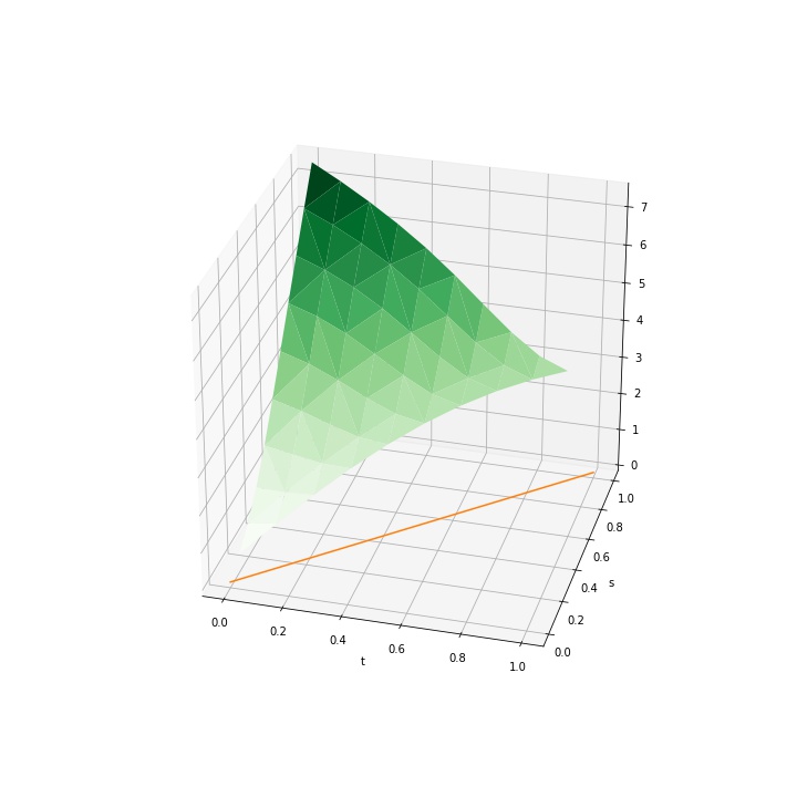
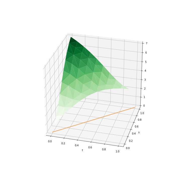
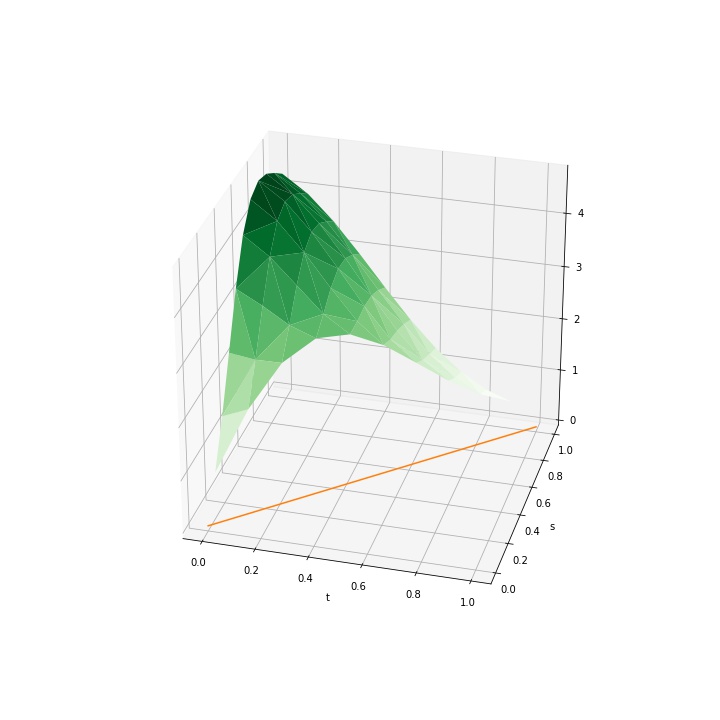
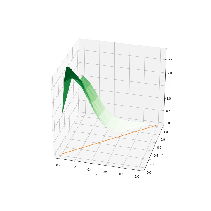
3.3 Simulation study

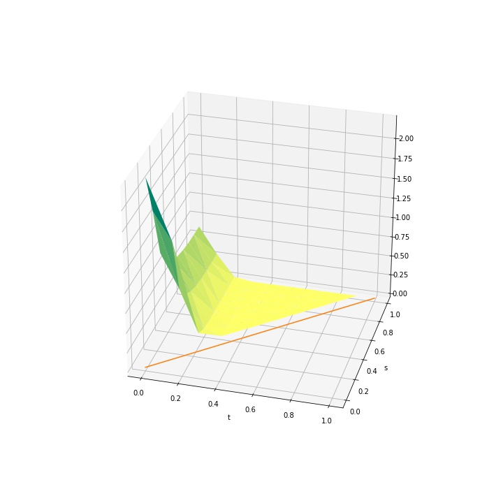
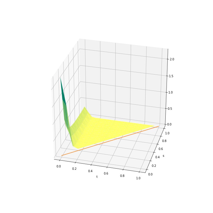
The aim of this section is to give an example of perturbations with ΔΡ​(t,s)β†’0,t<sformulae-sequenceβ†’subscriptΞ”πœ€π‘‘π‘ 0𝑑𝑠\Delta_{\varepsilon}(t,s)\rightarrow 0,\ t<s when $\varepsilon\rightarrow 0$, but $\left|b(t,x)-b_{\varepsilon}(t,x)\right|\not\rightarrow 0$ uniformly. The idea is to consider the case of highly oscillating perturbations when the integral is small for $\varepsilon\rightarrow 0$ , but the difference $\left|b(t,x)-b_{\varepsilon}(t,x)\right|$ remains of a constant order in the neighborhood of the point $t=\sqrt{\varepsilon}$. We consider the simplest case $d=\gamma=1$, ΔΡ,σ​(t,s)≑0subscriptΞ”πœ€πœŽπ‘‘π‘ 0\Delta_{\varepsilon,\sigma}(t,s)\equiv 0, and the drift perturbation of the following form:

$$b(t,x)=x,$$
$$b_{\varepsilon}(t,x)=b(t,x)+e^{-\frac{t^{2}}{q\varepsilon}}\sin^{\frac{2}{q}}\left(\frac{t}{\sqrt{\varepsilon}}\right)\cos(x).$$

Here, $q=\dfrac{p}{p-1},\ 2<q<\infty$. Clearly, in this case, (A) holds true. Let us estimate ΔΡ,b​(t,s)subscriptΞ”πœ€π‘π‘‘π‘ \Delta_{\varepsilon,b}(t,s) when $t<s$.

$$\displaystyle\left|b(t,x)-b_{\varepsilon}(t,x)\right|_{1}\leq e^{-\frac{t^{2}}{q\varepsilon}}\sin^{\frac{2}{q}}\left(\frac{t}{\sqrt{\varepsilon}}\right),$$
$$\Delta_{\varepsilon,b}(t,s)\leq\int_{t}^{s}\mathfrak{B}\left(u;1,\frac{1}{2}\right)\int_{\mathbb{R}^{d}}\int_{\mathbb{R}^{d}}\left|b\left(u,\theta_{u,s}(y)\right)-b_{\varepsilon}\left(u,\theta_{u,s}(y)\right)\right|_{1}\times$$
$$\times\bar{p}(t,s,x,y)dyd\mu(x)du\leq M\int_{t}^{s}\mathfrak{B}\left(u;1,\frac{1}{2}\right)e^{-\frac{u^{2}}{q\varepsilon}}\sin^{\frac{2}{q}}\left(\frac{u}{\sqrt{\varepsilon}}\right)du\leq$$
$$\leq M\left(\int_{t}^{s}\mathfrak{B}^{p}\left(u;1,\frac{1}{2}\right)du\right)^{\frac{1}{p}}\left(\int_{t}^{s}e^{-\frac{u^{2}}{\varepsilon}}\sin^{2}\left(\frac{u}{\sqrt{\varepsilon}}\right)du\right)^{\frac{1}{q}},\frac{1}{p}+\frac{1}{q}=1.$$

First,

$$\left(\int_{t}^{s}\mathfrak{B}^{p}\left(u;1,\frac{1}{2}\right)du\right)^{1/p}=\frac{1}{B\left(1,\frac{1}{2}\right)(s-t)^{\frac{1}{2}}}\left(\int_{t}^{s}(s-u)^{-\frac{p}{2}}du\right)^{1/p}=$$
$$=\frac{(s-t)^{\frac{1}{p}-1}}{B\left(1,\frac{1}{2}\right)\left(1-\frac{p}{2}\right)^{\frac{1}{p}}}.$$

Next, using the representation $\sin(x)=\dfrac{\exp(ix)-\exp(-ix)}{2i}$, we get:

$$\int_{0}^{\infty}e^{-x^{2}}\sin^{2}(x)dx=\int_{0}^{\infty}\left(\dfrac{e^{-x^{2}}}{2}-\dfrac{1}{4}e^{-(x-i)^{2}-1}-\dfrac{1}{4}e^{-(x+i)^{2}-1}\right)dx=\dfrac{\sqrt{\pi}}{4}\left(1-1/e\right).$$

As a consequence,

$$\left(\int_{t}^{s}e^{-\frac{u^{2}}{\varepsilon}}\sin^{2}\left(\frac{u}{\sqrt{\varepsilon}}\right)du\right)^{\frac{1}{q}}\leq\left(\int_{0}^{\infty}e^{-\frac{u^{2}}{\varepsilon}}\sin^{2}\left(\frac{u}{\sqrt{\varepsilon}}\right)du\right)^{\frac{1}{q}}=$$
$$=\left(\frac{1}{4}\sqrt{\pi\varepsilon}\left(1-1/e\right)\right)^{\frac{1}{q}}.$$

By Theorem 1.1,

β€–(pβˆ’pΞ΅)​(t,s,x,y)β€–L1μ​(ℝ,L1​(ℝ))≀subscriptnorm𝑝subscriptπ‘πœ€π‘‘π‘ π‘₯𝑦superscriptsubscript𝐿1πœ‡β„subscript𝐿1ℝabsent\left\|\left(p-p_{\varepsilon}\right)(t,s,x,y)\right\|_{L_{1}^{\mu}\left(\mathbb{R},L_{1}(\mathbb{R})\right)}\leq
$$\leq\frac{C}{\left(1-\frac{p}{2}\right)^{\frac{1}{p}}\left(\delta-\frac{1}{2}\right)}\left(\varepsilon^{k\left(\delta-\frac{1}{2}\right)}+\varepsilon^{\left(\frac{1}{2}-\kappa\right)\left(1-\frac{1}{p}\right)(1-\delta)}\right),$$

where $0<\kappa<\frac{1}{2},\frac{1}{2}<\delta<1,1<p<2.$

Equating the powers, we get for $\delta=\frac{3}{4},q=\frac{p-1}{p}>2$

β€–(pβˆ’pΞ΅)​(t,s,x,y)β€–L1μ​(ℝ,L1​(ℝ))≀subscriptnorm𝑝subscriptπ‘πœ€π‘‘π‘ π‘₯𝑦superscriptsubscript𝐿1πœ‡β„subscript𝐿1ℝabsent\left\|\left(p-p_{\varepsilon}\right)(t,s,x,y)\right\|_{L_{1}^{\mu}\left(\mathbb{R},L_{1}(\mathbb{R})\right)}\leq
$$\left.\frac{C}{\left(1-\frac{p}{2}\right)^{\frac{1}{p}}\left(\delta-\frac{1}{2}\right)}\varepsilon^{\frac{(1-\delta)\left(\delta-\frac{1}{2}\right)}{2\left[q\left(\delta-\frac{1}{2}\right)+1-\delta\right]}}\right|_{\delta=\frac{3}{4}}=\frac{C}{\left(1-\frac{p}{2}\right)^{\frac{1}{p}}}\varepsilon^{1/(8(1+q))}=\frac{C}{\left(1-\frac{p}{2}\right)^{\frac{1}{p}}}\varepsilon^{\frac{1}{24}-\rho}$$

for any $\rho>0$ and an appropriate choice of $q\rightarrow 2+$.

Importantly, the perturbation does not tend to zero uniformly. Indeed, for $\frac{\pi\sqrt{\varepsilon}}{6}\leq t\leq\frac{\pi\sqrt{\varepsilon}}{2}$,

$$\left|b_{\varepsilon}(t,x)-b(t,x)\right|\geq 2^{-\frac{2}{q}}e^{-\frac{\pi^{2}}{4q}}\left|\cos(x)\right|.$$

The following numerical experiments demonstrate the behavior of the perturbation argument ΔΡ,b​(t,s)subscriptΞ”πœ€π‘π‘‘π‘ \Delta_{\varepsilon,b}(t,s) in the neighborhood of the point $t=\sqrt{\varepsilon}$ for different $\varepsilon$. We consider the time step $\Delta t$, the constant $q=2.01$ and the probability measure $\mu(\cdot)=\delta_{1}(\cdot)$, where $\delta_{x}(\cdot)$ is a Dirac delta measure centred on some fixed point $x\in\mathbb{R}$.

Refer to caption
Figure 1: $\Delta_{\varepsilon,b}(t,s),\ 0\leq t<s\leq 1,$
Β Β Β Β Β Β Β Β Β Β Β Β Β Β Β Β Β Β Β Β Β Β Β Β Β Β Β Β Β Β Β Β Β Β Β Β Β Β Β Β Β Β Β Β Β Β Β Β Β Β Β Β Β Β Β Β Β Β Β Β Β Β Β Β Β Β Β Β Β Β Β Β Β Β Β Β Β Β Β Β Β Β Β Β Β Β Β Β Β Β Β Β Β Β Β Β Β Β Β Β Β Β Β Β Β Β Β Β Β Β Β Β Β Β Β Β Β Β Β Β Β Β Β Β Β Β Β Β Β Β Β Β Β Β Β Β Β Β Β Β Β Β Β Β Β  where $\Delta t=0.1,\ \varepsilon=1.$
Refer to caption
Figure 2: $\Delta_{\varepsilon,b}(t,s),\ 0\leq t<s\leq 1,$
Β Β Β Β Β Β Β Β Β Β Β Β Β Β Β Β Β Β Β Β Β Β Β Β Β Β Β Β Β Β Β Β Β Β Β Β Β Β Β Β Β Β Β Β Β Β Β Β Β Β Β Β Β Β Β Β Β Β Β Β Β Β Β Β Β Β Β Β Β Β Β Β Β Β Β Β Β Β Β Β Β Β Β Β Β Β Β Β Β Β Β Β Β Β Β Β Β Β Β Β Β Β Β Β Β Β Β Β Β Β Β Β Β Β Β Β Β Β Β Β Β Β Β Β Β Β Β Β Β Β Β Β Β Β Β Β Β Β Β Β Β Β Β Β Β  where $\Delta t=0.1,\ \varepsilon=0.5.$
Refer to caption
Figure 3: $\Delta_{\varepsilon,b}(t,s),\ 0\leq t<s\leq 1,$
Β Β Β Β Β Β Β Β Β Β Β Β Β Β Β Β Β Β Β Β Β Β Β Β Β Β Β Β Β Β Β Β Β Β Β Β Β Β Β Β Β Β Β Β Β Β Β Β Β Β Β Β Β Β Β Β Β Β Β Β Β Β Β Β Β Β Β Β Β Β Β Β Β Β Β Β Β Β Β Β Β Β Β Β Β Β Β Β Β Β Β Β Β Β Β Β Β Β Β Β Β Β Β Β Β Β Β Β Β Β Β Β Β Β Β Β Β Β Β Β Β Β Β Β Β Β Β Β Β Β Β Β Β Β Β Β Β Β Β Β Β Β Β Β Β  where $\Delta t=0.1,\ \varepsilon=0.2.$
Refer to caption
Figure 4: $\Delta_{\varepsilon,b}(t,s),\ 0\leq t<s\leq 1,$
Β Β Β Β Β Β Β Β Β Β Β Β Β Β Β Β Β Β Β Β Β Β Β Β Β Β Β Β Β Β Β Β Β Β Β Β Β Β Β Β Β Β Β Β Β Β Β Β Β Β Β Β Β Β Β Β Β Β Β Β Β Β Β Β Β Β Β Β Β Β Β Β Β Β Β Β Β Β Β Β Β Β Β Β Β Β Β Β Β Β Β Β Β Β Β Β Β Β Β Β Β Β Β Β Β Β Β Β Β Β Β Β Β Β Β Β Β Β Β Β Β Β Β Β Β Β Β Β Β Β Β Β Β Β Β Β Β Β Β Β Β Β Β Β Β  where $\Delta t=0.1,\ \varepsilon=0.05.$
Refer to caption
Figure 5: $\Delta_{\varepsilon,b}(t,s),\ 0\leq t<s\leq 1,$
Β Β Β Β Β Β Β Β Β Β Β Β Β Β Β Β Β Β Β Β Β Β Β Β Β Β Β Β Β Β Β Β Β Β Β Β Β Β Β Β Β Β Β Β Β Β Β Β Β Β Β Β Β Β Β Β Β Β Β Β Β Β Β Β Β Β Β Β Β Β Β Β Β Β Β Β Β Β Β Β Β Β Β Β Β Β Β Β Β Β Β Β Β Β Β Β Β Β Β Β Β Β Β Β Β Β Β Β Β Β Β Β Β Β Β Β Β Β Β Β Β Β Β Β Β Β Β Β Β Β Β Β Β Β Β Β Β Β Β Β Β Β Β Β Β  where $\Delta t=0.1,\ \varepsilon=0.01.$
Refer to caption
Figure 6: $\Delta_{\varepsilon,b}(t,s),\ 0\leq t<s\leq 1,$
Β Β Β Β Β Β Β Β Β Β Β Β Β Β Β Β Β Β Β Β Β Β Β Β Β Β Β Β Β Β Β Β Β Β Β Β Β Β Β Β Β Β Β Β Β Β Β Β Β Β Β Β Β Β Β Β Β Β Β Β Β Β Β Β Β Β Β Β Β Β Β Β Β Β Β Β Β Β Β Β Β Β Β Β Β Β Β Β Β Β Β Β Β Β Β Β Β Β Β Β Β Β Β Β Β Β Β Β Β Β Β Β Β Β Β Β Β Β Β Β Β Β Β Β Β Β Β Β Β Β Β Β Β Β Β Β Β Β Β Β Β Β Β Β Β  where $\Delta t=0.05,\ \varepsilon=0.0025.$

4 Appendix

4.1 Proof of Lemma 3.1

Let us consider the case when $|\nu|=0$. Let us now identify the transition densities $\widetilde{p}(t,s,x,y)$ and p~Ρ​(t,s,x,y)subscript~π‘πœ€π‘‘π‘ π‘₯𝑦\widetilde{p}_{\varepsilon}(t,s,x,y) with $(d+1)\times d$ matrices $\Omega$ and $\Omega^{\varepsilon}$ consisting of the first rows that are the components of the respective mean vectors ΞΈt,s​(y)=(ΞΈt,s1​(y),…,ΞΈt,sd​(y))subscriptπœƒπ‘‘π‘ π‘¦subscriptsuperscriptπœƒ1𝑑𝑠𝑦…subscriptsuperscriptπœƒπ‘‘π‘‘π‘ π‘¦\theta_{t,s}(y)=\left(\theta^{1}_{t,s}(y),\dots,\theta^{d}_{t,s}(y)\right) and ΞΈt,sΡ​(y)=(ΞΈt,s1,Ρ​(y),…,ΞΈt,sd,Ρ​(y))subscriptsuperscriptπœƒπœ€π‘‘π‘ π‘¦subscriptsuperscriptπœƒ1πœ€π‘‘π‘ π‘¦β€¦subscriptsuperscriptπœƒπ‘‘πœ€π‘‘π‘ π‘¦\theta^{\varepsilon}_{t,s}(y)=\left(\theta^{1,\varepsilon}_{t,s}(y),\dots,\theta^{d,\varepsilon}_{t,s}(y)\right), and the $d\times d$ covariance matrices, namely, Ξ©i​j=∫tsai​j​(u,ΞΈu,s​(y))​𝑑u,Ξ©i​jΞ΅=∫tsaΞ΅i​j​(u,ΞΈu,sΡ​(y))​𝑑uformulae-sequencesubscriptΩ𝑖𝑗superscriptsubscript𝑑𝑠subscriptπ‘Žπ‘–π‘—π‘’subscriptπœƒπ‘’π‘ π‘¦differential-d𝑒subscriptsuperscriptΞ©πœ€π‘–π‘—superscriptsubscript𝑑𝑠superscriptsubscriptπ‘Žπœ€π‘–π‘—π‘’subscriptsuperscriptπœƒπœ€π‘’π‘ π‘¦differential-d𝑒\Omega_{ij}=\int_{t}^{s}a_{ij}(u,\theta_{u,s}(y))du,\ \Omega^{\varepsilon}_{ij}=\int_{t}^{s}a_{\varepsilon}^{ij}(u,\theta^{\varepsilon}_{u,s}(y))du, where $i>1$.


For $(d+1)\times d$ matrix $A$, we will denote by $A_{1}$ the first row and by $A_{2:d+1}$ the square matrix composed of rows from $2$ to $d+1$.

We can rewrite $\widetilde{p}(t,s,x,y)$ and p~Ρ​(t,s,x,y)subscript~π‘πœ€π‘‘π‘ π‘₯𝑦\widetilde{p}_{\varepsilon}(t,s,x,y) in terms of $\Omega$ and $\Omega^{\varepsilon}$:

$\displaystyle\widetilde{p}(t,s,x,y)=f\left(\Omega\right),$
p~Ρ​(t,s,x,y)=f​(ΩΡ),subscript~π‘πœ€π‘‘π‘ π‘₯𝑦𝑓superscriptΞ©πœ€\displaystyle\widetilde{p}_{\varepsilon}(t,s,x,y)=f\left(\Omega^{\varepsilon}\right),

where

$\displaystyle f:\mathbb{R}^{(d+1)\times d}\rightarrow\mathbb{R},$
$\displaystyle A\mapsto f(A)=\dfrac{1}{(2\pi)^{d/2}\operatorname{det}(A_{2:d+1})^{1/2}}$ $\displaystyle\exp\left(-\dfrac{1}{2}\langle(A_{2:d+1})^{-1}(A_{1}-x),A_{1}-x\rangle\right).$

So, applying the Taylor expansion and (2.16) combined with (A4) gives:

$$|\widetilde{p}_{\varepsilon}-\widetilde{p}|(t,s,x,y)=\left|f(\Omega)-f(\Omega_{\varepsilon})\right|=$$
$$=\left|\sum\limits_{|\nu|=1}\left(\Omega_{\varepsilon}-\Omega\right)^{\nu}\cdot\int\limits_{0}^{1}(1-\lambda)\mathcal{D}^{\nu}f\left\{\Omega+\lambda(\Omega_{\varepsilon}-\Omega)\right\}d\lambda\right|=$$
$$=\left|\sum\limits_{i=1}^{d}\left(\theta^{i,\varepsilon}_{t,s}(y)-\theta^{i}_{t,s}(y)\right)\cdot\int\limits_{0}^{1}(1-\lambda)\mathcal{D}^{\nu_{1}^{i}}f\left\{\Omega+\lambda(\Omega_{\varepsilon}-\Omega)\right\}d\lambda+\right.$$
+βˆ‘i,j=1d(∫tsai​jΡ​(u,ΞΈu,sΡ​(y))​𝑑uβˆ’βˆ«tsai​j​(u,ΞΈu,sΡ​(y))​𝑑u)β‹…βˆ«01(1βˆ’Ξ»)β€‹π’ŸΞ½2:d+1i​j​f​{Ξ©+λ​(Ξ©Ξ΅βˆ’Ξ©)}​𝑑λ|≀conditionalsuperscriptsubscript𝑖𝑗1𝑑⋅superscriptsubscript𝑑𝑠subscriptsuperscriptπ‘Žπœ€π‘–π‘—π‘’subscriptsuperscriptπœƒπœ€π‘’π‘ π‘¦differential-d𝑒superscriptsubscript𝑑𝑠subscriptπ‘Žπ‘–π‘—π‘’subscriptsuperscriptπœƒπœ€π‘’π‘ π‘¦differential-d𝑒superscriptsubscript011πœ†superscriptπ’Ÿsuperscriptsubscript𝜈:2𝑑1π‘–π‘—π‘“Ξ©πœ†subscriptΞ©πœ€Ξ©differential-dπœ†\left.+\sum\limits_{i,j=1}^{d}\left(\int_{t}^{s}a^{\varepsilon}_{ij}(u,\theta^{\varepsilon}_{u,s}(y))du-\int_{t}^{s}a_{ij}(u,\theta^{\varepsilon}_{u,s}(y))du\right)\cdot\int\limits_{0}^{1}(1-\lambda)\mathcal{D}^{\nu_{2:d+1}^{ij}}f\left\{\Omega+\lambda(\Omega_{\varepsilon}-\Omega)\right\}d\lambda\right|\leq
≀C(sβˆ’t)(1+d)/2​exp⁑(βˆ’|ΞΈt,s​(y)+c​(ΞΈt,sΡ​(y)βˆ’ΞΈt,s​(y))βˆ’x|2C​(sβˆ’t))β‹…(|ΞΈt,sΡ​(y)βˆ’ΞΈt,s​(y)|)+absentlimit-from⋅𝐢superscript𝑠𝑑1𝑑2superscriptsubscriptπœƒπ‘‘π‘ π‘¦π‘superscriptsubscriptπœƒπ‘‘π‘ πœ€π‘¦subscriptπœƒπ‘‘π‘ π‘¦π‘₯2𝐢𝑠𝑑superscriptsubscriptπœƒπ‘‘π‘ πœ€π‘¦subscriptπœƒπ‘‘π‘ π‘¦\leq\dfrac{C}{\left({s-t}\right)^{(1+d)/2}}\exp\left(\dfrac{-\left|\theta_{t,s}(y)+c(\theta_{t,s}^{\varepsilon}(y)-\theta_{t,s}(y))-x\right|^{2}}{C(s-t)}\right)\cdot\left(\left|\theta_{t,s}^{\varepsilon}(y)-\theta_{t,s}(y)\right|\right)+
+C(sβˆ’t)1+d/2​exp⁑(βˆ’|ΞΈt,s​(y)+c​(ΞΈt,sΡ​(y)βˆ’ΞΈt,s​(y))βˆ’x|2C​(sβˆ’t))β‹…(∫ts|a​(u,ΞΈu,s​(y))βˆ’aΡ​(u,ΞΈu,sΡ​(y))|​𝑑u)≀⋅𝐢superscript𝑠𝑑1𝑑2superscriptsubscriptπœƒπ‘‘π‘ π‘¦π‘superscriptsubscriptπœƒπ‘‘π‘ πœ€π‘¦subscriptπœƒπ‘‘π‘ π‘¦π‘₯2𝐢𝑠𝑑superscriptsubscriptπ‘‘π‘ π‘Žπ‘’subscriptπœƒπ‘’π‘ π‘¦subscriptπ‘Žπœ€π‘’subscriptsuperscriptπœƒπœ€π‘’π‘ π‘¦differential-d𝑒absent+\dfrac{C}{\left({s-t}\right)^{1+d/2}}\exp\left(\dfrac{-\left|\theta_{t,s}(y)+c(\theta_{t,s}^{\varepsilon}(y)-\theta_{t,s}(y))-x\right|^{2}}{C(s-t)}\right)\cdot\left(\int_{t}^{s}\left|a(u,\theta_{u,s}(y))-a_{\varepsilon}(u,\theta^{\varepsilon}_{u,s}(y))\right|du\right)\leq
≀C(sβˆ’t)1/2​p¯​(t,s,x,y)​exp⁑(c​|ΞΈt,sΡ​(y)βˆ’ΞΈt,s​(y)|2C​(sβˆ’t))​(∫ts|(bβˆ’bΞ΅)​(u,ΞΈu,s​(y))|​𝑑u)+absentlimit-from𝐢superscript𝑠𝑑12¯𝑝𝑑𝑠π‘₯𝑦𝑐superscriptsuperscriptsubscriptπœƒπ‘‘π‘ πœ€π‘¦subscriptπœƒπ‘‘π‘ π‘¦2𝐢𝑠𝑑superscriptsubscript𝑑𝑠𝑏subscriptπ‘πœ€π‘’subscriptπœƒπ‘’π‘ π‘¦differential-d𝑒\leq\dfrac{C}{\left({s-t}\right)^{1/2}}\bar{p}(t,s,x,y)\exp\left(\frac{c\left|\theta_{t,s}^{\varepsilon}(y)-\theta_{t,s}(y)\right|^{2}}{C(s-t)}\right)\left(\int_{t}^{s}\left|\left(b-b_{\varepsilon}\right)\left(u,\theta_{u,s}(y)\right)\right|du\right)+
$$+\dfrac{C}{\left({s-t}\right)}\bar{p}(t,s,x,y)\exp\left(\frac{c\left|\theta_{t,s}^{\varepsilon}(y)-\theta_{t,s}(y)\right|^{2}}{C(s-t)}\right)\left((s-t)\left(\int_{t}^{s}\left|\left(b-b_{\varepsilon}\right)\left(u,\theta_{u,s}(y)\right)\right|du\right)^{\gamma}+\right.$$
$$\left.+\int_{t}^{s}\left|\left(\sigma-\sigma_{\varepsilon}\right)\left(u,\theta_{u,s}(y)\right)\right|du\right)\leq$$
≀C​p¯​(t,s,x,y)​((∫ts|(bβˆ’bΞ΅)​(u,ΞΈu,s​(y))|​𝑑u)Ξ³(sβˆ’t)Ξ³/2+(∫ts|(Οƒβˆ’ΟƒΞ΅)​(u,ΞΈu,s​(y))|​𝑑u)Ξ³(sβˆ’t)Ξ³).absent𝐢¯𝑝𝑑𝑠π‘₯𝑦superscriptsuperscriptsubscript𝑑𝑠𝑏subscriptπ‘πœ€π‘’subscriptπœƒπ‘’π‘ π‘¦differential-d𝑒𝛾superscript𝑠𝑑𝛾2superscriptsuperscriptsubscriptπ‘‘π‘ πœŽsubscriptπœŽπœ€π‘’subscriptπœƒπ‘’π‘ π‘¦differential-d𝑒𝛾superscript𝑠𝑑𝛾\leq C\bar{p}(t,s,x,y)\left(\dfrac{\left(\int_{t}^{s}\left|\left(b-b_{\varepsilon}\right)\left(u,\theta_{u,s}(y)\right)\right|du\right)^{\gamma}}{(s-t)^{\gamma/2}}+\dfrac{\left(\int_{t}^{s}\left|\left(\sigma-\sigma_{\varepsilon}\right)\left(u,\theta_{u,s}(y)\right)\right|du\right)^{\gamma}}{(s-t)^{\gamma}}\right).

We will use a slightly different bound:

$$|\widetilde{p}_{\varepsilon}-\widetilde{p}|(t,s,x,y)\leq$$
≀C​p¯​(t,s,x,y)​((∫ts|(bβˆ’bΞ΅)​(u,ΞΈu,s​(y))|​𝑑u)Ξ³βˆ’Ξ΄(sβˆ’t)Ξ³/2βˆ’Ξ΄/2+(∫ts|(Οƒβˆ’ΟƒΞ΅)​(u,ΞΈu,s​(y))|​𝑑u)Ξ³βˆ’Ξ΄(sβˆ’t)Ξ³βˆ’Ξ΄).absent𝐢¯𝑝𝑑𝑠π‘₯𝑦superscriptsuperscriptsubscript𝑑𝑠𝑏superscriptπ‘πœ€π‘’subscriptπœƒπ‘’π‘ π‘¦differential-d𝑒𝛾𝛿superscript𝑠𝑑𝛾2𝛿2superscriptsuperscriptsubscriptπ‘‘π‘ πœŽsuperscriptπœŽπœ€π‘’subscriptπœƒπ‘’π‘ π‘¦differential-d𝑒𝛾𝛿superscript𝑠𝑑𝛾𝛿\leq C\bar{p}(t,s,x,y)\left(\dfrac{\left(\int_{t}^{s}\left|\left(b-b^{\varepsilon}\right)\left(u,\theta_{u,s}(y)\right)\right|du\right)^{\gamma-\delta}}{(s-t)^{\gamma/2-\delta/2}}+\dfrac{\left(\int_{t}^{s}\left|\left(\sigma-\sigma^{\varepsilon}\right)\left(u,\theta_{u,s}(y)\right)\right|du\right)^{\gamma-\delta}}{(s-t)^{\gamma-\delta}}\right). (4.1)

Now the upper bound on the difference in $L_{1}-L_{1}$ norm easily follows from (4.1) and Jensen’s inequality:

$$||\left(\widetilde{p}_{\varepsilon}-\widetilde{p}\right)(t,s,x,y)||_{L_{1}^{\mu}({\mathbb{R}^{d}},L_{1}(\mathbb{R}^{d}))}\leq$$
≀C(sβˆ’t)Ξ³βˆ’Ξ΄β€‹βˆ«β„dβˆ«β„dp¯​(t,s,x,y)⋅φ​(t,s;y)​𝑑y​μ​(d​x)≀absent𝐢superscript𝑠𝑑𝛾𝛿subscriptsuperscriptℝ𝑑subscriptsuperscriptℝ𝑑⋅¯𝑝𝑑𝑠π‘₯π‘¦πœ‘π‘‘π‘ π‘¦differential-dπ‘¦πœ‡π‘‘π‘₯absent\leq\dfrac{C}{(s-t)^{\gamma-\delta}}\int\limits_{\mathbb{R}^{d}}\int\limits_{\mathbb{R}^{d}}\bar{p}(t,s,x,y)\cdot{\varphi}(t,s;y)dy\ \mu(dx)\leq
$$\leq C\left[\left(\int_{\mathbb{R}^{d}}\int_{\mathbb{R}^{d}}\int_{t}^{s}\mathfrak{B}(u;1,\gamma/2)\left|\left(b-b_{\varepsilon}\right)\left(u,\theta_{u,s}(y)\right)\right|_{1}\bar{p}(t,s,x,y)dudy\ \mu(dx)\right)^{\gamma-\delta}\right.+$$
$$+\left.\left(\int_{\mathbb{R}^{d}}\int_{\mathbb{R}^{d}}\int_{t}^{s}\mathfrak{B}(u;1,\gamma/2)\left|\left(\sigma-\sigma_{\varepsilon}\right)\left(u,\theta_{u,s}(y)\right)\right|_{\gamma}\bar{p}(t,s,x,y)dudy\ \mu(dx)\right)^{\gamma-\delta}\right]=$$
$$=C\left[\left(\Delta_{\varepsilon,b}\right)^{\gamma-\delta}+\left(\Delta_{\varepsilon,\sigma}\right)^{\gamma-\delta}\right].$$

The bounds for $|\nu|\geq 1$ follow from differentiation of the Taylor expansion and similar bounds (2.16) for the derivatives of the Gaussian densities $\widetilde{p}$ and $\widetilde{p}_{\varepsilon}$.

4.2 Proof of Lemma 3.2

In order to prove the Lemma 3.2, we decompose the difference |Hβˆ’HΞ΅|​(t,s,x,y)𝐻subscriptπ»πœ€π‘‘π‘ π‘₯𝑦\left|H-H_{\varepsilon}\right|(t,s,x,y) into 6 parts in the following way:

|Hβˆ’HΞ΅|​(t,s,x,y)≀𝐻subscriptπ»πœ€π‘‘π‘ π‘₯𝑦absent\displaystyle\left|H-H_{\varepsilon}\right|(t,s,x,y)\leq (4.2)
≀12β€‹βˆ‘i,j=1d|ai​j​(t,x)βˆ’ai​jΡ​(t,x)βˆ’ai​j​(t,ΞΈt,s​(y))+ai​jΡ​(t,ΞΈt,s​(y))|​|βˆ‚2p~​(t,s,x,y)βˆ‚xiβ€‹βˆ‚xj|+absentlimit-from12superscriptsubscript𝑖𝑗1𝑑subscriptπ‘Žπ‘–π‘—π‘‘π‘₯superscriptsubscriptπ‘Žπ‘–π‘—πœ€π‘‘π‘₯subscriptπ‘Žπ‘–π‘—π‘‘subscriptπœƒπ‘‘π‘ π‘¦superscriptsubscriptπ‘Žπ‘–π‘—πœ€π‘‘subscriptπœƒπ‘‘π‘ π‘¦superscript2~𝑝𝑑𝑠π‘₯𝑦subscriptπ‘₯𝑖subscriptπ‘₯𝑗\displaystyle\leq\dfrac{1}{2}\sum_{i,j=1}^{d}\left|a_{ij}(t,x)-a_{ij}^{\varepsilon}(t,x)-a_{ij}(t,\theta_{t,s}(y))+a_{ij}^{\varepsilon}(t,\theta_{t,s}(y))\right|\left|\dfrac{\partial^{2}\widetilde{p}(t,s,x,y)}{\partial x_{i}\partial x_{j}}\right|+ (4.3)
+12β€‹βˆ‘i,j=1d|ai​jΡ​(t,ΞΈt,sΡ​(y))βˆ’ai​jΡ​(t,ΞΈt,s​(y))|​|βˆ‚2p~​(t,s,x,y)βˆ‚xiβ€‹βˆ‚xj|+limit-from12superscriptsubscript𝑖𝑗1𝑑superscriptsubscriptπ‘Žπ‘–π‘—πœ€π‘‘subscriptsuperscriptπœƒπœ€π‘‘π‘ π‘¦superscriptsubscriptπ‘Žπ‘–π‘—πœ€π‘‘subscriptπœƒπ‘‘π‘ π‘¦superscript2~𝑝𝑑𝑠π‘₯𝑦subscriptπ‘₯𝑖subscriptπ‘₯𝑗\displaystyle+\dfrac{1}{2}\sum_{i,j=1}^{d}\left|a_{ij}^{\varepsilon}(t,\theta^{\varepsilon}_{t,s}(y))-a_{ij}^{\varepsilon}(t,\theta_{t,s}(y))\right|\left|\dfrac{\partial^{2}\widetilde{p}(t,s,x,y)}{\partial x_{i}\partial x_{j}}\right|+ (4.4)
+12β€‹βˆ‘i,j=1d|ai​jΡ​(t,x)βˆ’ai​jΡ​(t,ΞΈt,sΡ​(y))|​|βˆ‚2(p~​(t,s,x,y)βˆ’p~Ρ​(t,s,x,y))βˆ‚xiβ€‹βˆ‚xj|+limit-from12superscriptsubscript𝑖𝑗1𝑑superscriptsubscriptπ‘Žπ‘–π‘—πœ€π‘‘π‘₯superscriptsubscriptπ‘Žπ‘–π‘—πœ€π‘‘subscriptsuperscriptπœƒπœ€π‘‘π‘ π‘¦superscript2~𝑝𝑑𝑠π‘₯𝑦subscript~π‘πœ€π‘‘π‘ π‘₯𝑦subscriptπ‘₯𝑖subscriptπ‘₯𝑗\displaystyle+\dfrac{1}{2}\sum_{i,j=1}^{d}\left|a_{ij}^{\varepsilon}(t,x)-a_{ij}^{\varepsilon}(t,\theta^{\varepsilon}_{t,s}(y))\right|\left|\dfrac{\partial^{2}\left(\widetilde{p}(t,s,x,y)-\widetilde{p}_{\varepsilon}(t,s,x,y)\right)}{\partial x_{i}\partial x_{j}}\right|+ (4.5)
+βˆ‘i=1d|bi​(t,x)βˆ’bi​(t,ΞΈt,s​(y))βˆ’biΡ​(t,x)+biΡ​(t,ΞΈt,s​(y))|​|βˆ‚p~​(t,s,x,y)βˆ‚xi|+limit-fromsuperscriptsubscript𝑖1𝑑subscript𝑏𝑖𝑑π‘₯subscript𝑏𝑖𝑑subscriptπœƒπ‘‘π‘ π‘¦superscriptsubscriptπ‘π‘–πœ€π‘‘π‘₯superscriptsubscriptπ‘π‘–πœ€π‘‘subscriptπœƒπ‘‘π‘ π‘¦~𝑝𝑑𝑠π‘₯𝑦subscriptπ‘₯𝑖\displaystyle+\sum_{i=1}^{d}\left|b_{i}(t,x)-b_{i}(t,\theta_{t,s}(y))-b_{i}^{\varepsilon}(t,x)+b_{i}^{\varepsilon}(t,\theta_{t,s}(y))\right|\left|\dfrac{\partial\widetilde{p}(t,s,x,y)}{\partial x_{i}}\right|+ (4.6)
+βˆ‘i=1d|biΡ​(t,ΞΈt,sΡ​(y))βˆ’biΡ​(t,ΞΈt,s​(y))|​|βˆ‚p~​(t,s,x,y)βˆ‚xi|+limit-fromsuperscriptsubscript𝑖1𝑑superscriptsubscriptπ‘π‘–πœ€π‘‘subscriptsuperscriptπœƒπœ€π‘‘π‘ π‘¦superscriptsubscriptπ‘π‘–πœ€π‘‘subscriptπœƒπ‘‘π‘ π‘¦~𝑝𝑑𝑠π‘₯𝑦subscriptπ‘₯𝑖\displaystyle+\sum_{i=1}^{d}\left|b_{i}^{\varepsilon}(t,\theta^{\varepsilon}_{t,s}(y))-b_{i}^{\varepsilon}(t,\theta_{t,s}(y))\right|\left|\dfrac{\partial\widetilde{p}(t,s,x,y)}{\partial x_{i}}\right|+ (4.7)
$$\displaystyle+\sum_{i=1}^{d}\left|b_{i}^{\varepsilon}(t,x)-b_{i}^{\varepsilon}(t,\theta^{\varepsilon}_{t,s}(y))\right|\left|\dfrac{\partial\left(\widetilde{p}-\widetilde{p}_{\varepsilon}\right)(t,s,x,y)}{\partial x_{i}}\right|:=i)+ii)+iii)+iv)+v)+vi).$$ (4.8)

For $ii)$ and $v)$, by regularity assumptions and (2.16), we have

$$ii)\leq\dfrac{C}{s-t}\bar{p}(t,s,x,y)\left|\theta^{\varepsilon}_{t,s}(y)-\theta_{t,s}(y)\right|^{\gamma}\leq\dfrac{C}{(s-t)^{1-\delta/2}}\bar{p}(t,s,x,y)\left(\int_{t}^{s}\left|\left(b-b^{\varepsilon}\right)\left(u,\theta_{u,s}(y)\right)\right|_{1}du\right)^{\gamma-\delta}.$$
$$v)\leq\dfrac{C}{(s-t)^{1/2}}\bar{p}(t,s,x,y)\left|\theta^{\varepsilon}_{t,s}(y)-\theta_{t,s}(y)\right|\leq\dfrac{C}{(s-t)^{1/2}}\bar{p}(t,s,x,y)\left(\int_{t}^{s}\left|\left(b-b^{\varepsilon}\right)\left(u,\theta_{u,s}(y)\right)\right|_{1}du\right).$$

To obtain an upper bound for $i)$, we first estimate the first part of the corresponding expression:

|a​(t,x)βˆ’aΡ​(t,x)βˆ’a​(t,ΞΈt,s​(y))+aΡ​(t,ΞΈt,s​(y))|=π‘Žπ‘‘π‘₯superscriptπ‘Žπœ€π‘‘π‘₯π‘Žπ‘‘subscriptπœƒπ‘‘π‘ π‘¦superscriptπ‘Žπœ€π‘‘subscriptπœƒπ‘‘π‘ π‘¦absent\left|a(t,x)-a^{\varepsilon}(t,x)-a(t,\theta_{t,s}(y))+a^{\varepsilon}(t,\theta_{t,s}(y))\right|=
=|Οƒβ€‹Οƒβˆ—β€‹(t,x)βˆ’ΟƒΞ΅β€‹(σΡ)βˆ—β€‹(t,x)βˆ’Οƒβ€‹Οƒβˆ—β€‹(t,ΞΈt,s​(y))+σΡ​(σΡ)βˆ—β€‹(t,ΞΈt,s​(y))|≀absent𝜎superscriptπœŽπ‘‘π‘₯superscriptπœŽπœ€superscriptsuperscriptπœŽπœ€π‘‘π‘₯𝜎superscriptπœŽπ‘‘subscriptπœƒπ‘‘π‘ π‘¦superscriptπœŽπœ€superscriptsuperscriptπœŽπœ€π‘‘subscriptπœƒπ‘‘π‘ π‘¦absent=\left|\sigma\sigma^{*}(t,x)-\sigma^{\varepsilon}(\sigma^{\varepsilon})^{*}(t,x)-\sigma\sigma^{*}(t,\theta_{t,s}(y))+\sigma^{\varepsilon}(\sigma^{\varepsilon})^{*}(t,\theta_{t,s}(y))\right|\leq
$$\leq\left[\left|\sigma(t,x)-\sigma^{\varepsilon}(t,x)-\left(\sigma(t,\theta_{t,s}(y))-\sigma^{\varepsilon}(t,\theta_{t,s}(y))\right)\right|\left|\sigma^{*}(t,x)\right|+\right.$$
+|σ​(t,x)βˆ’ΟƒΞ΅β€‹(t,x)βˆ’(σ​(t,ΞΈt,s​(y))βˆ’ΟƒΞ΅β€‹(t,ΞΈt,s​(y)))|​|(σΡ)βˆ—β€‹(t,x)|+limit-fromπœŽπ‘‘π‘₯superscriptπœŽπœ€π‘‘π‘₯πœŽπ‘‘subscriptπœƒπ‘‘π‘ π‘¦superscriptπœŽπœ€π‘‘subscriptπœƒπ‘‘π‘ π‘¦superscriptsuperscriptπœŽπœ€π‘‘π‘₯+\left|\sigma(t,x)-\sigma^{\varepsilon}(t,x)-\left(\sigma(t,\theta_{t,s}(y))-\sigma^{\varepsilon}(t,\theta_{t,s}(y))\right)\right|\left|(\sigma^{\varepsilon})^{*}(t,x)\right|+
+|Οƒβˆ—β€‹(t,x)βˆ’(σΡ)βˆ—β€‹(t,x)βˆ’(Οƒβˆ—β€‹(t,ΞΈt,s​(y))βˆ’(σΡ)βˆ—β€‹(t,ΞΈt,s​(y)))|​|σ​(t,ΞΈt,s​(y))|+limit-fromsuperscriptπœŽπ‘‘π‘₯superscriptsuperscriptπœŽπœ€π‘‘π‘₯superscriptπœŽπ‘‘subscriptπœƒπ‘‘π‘ π‘¦superscriptsuperscriptπœŽπœ€π‘‘subscriptπœƒπ‘‘π‘ π‘¦πœŽπ‘‘subscriptπœƒπ‘‘π‘ π‘¦+\left|\sigma^{*}(t,x)-(\sigma^{\varepsilon})^{*}(t,x)-\left(\sigma^{*}(t,\theta_{t,s}(y))-(\sigma^{\varepsilon})^{*}(t,\theta_{t,s}(y))\right)\right|\left|\sigma(t,\theta_{t,s}(y))\right|+
+|σ​(t,ΞΈt,s​(y))βˆ’ΟƒΞ΅β€‹(t,ΞΈt,s​(y))|​|(σΡ)βˆ—β€‹(t,x)βˆ’(σΡ)βˆ—β€‹(t,ΞΈt,s​(y))|+limit-fromπœŽπ‘‘subscriptπœƒπ‘‘π‘ π‘¦superscriptπœŽπœ€π‘‘subscriptπœƒπ‘‘π‘ π‘¦superscriptsuperscriptπœŽπœ€π‘‘π‘₯superscriptsuperscriptπœŽπœ€π‘‘subscriptπœƒπ‘‘π‘ π‘¦\left.+\left|\sigma(t,\theta_{t,s}(y))-\sigma^{\varepsilon}(t,\theta_{t,s}(y))\right|\left|(\sigma^{\varepsilon})^{*}(t,x)-(\sigma^{\varepsilon})^{*}(t,\theta_{t,s}(y))\right|+\right.
$$\left.+\left|\sigma^{\varepsilon}(t,x)-\sigma^{\varepsilon}(t,\theta_{t,s}(y))\right|\left|\sigma^{*}(t,x)-(\sigma^{\varepsilon})^{*}(t,x)\right|\right]\leq$$
≀C​(|xβˆ’ΞΈt,s​(y)|Ξ³+|xβˆ’ΞΈt,s​(y)|2​γ)​|(Οƒβˆ’ΟƒΞ΅)​(t,ΞΈt,s​(y))|Ξ³.absent𝐢superscriptπ‘₯subscriptπœƒπ‘‘π‘ π‘¦π›Ύsuperscriptπ‘₯subscriptπœƒπ‘‘π‘ π‘¦2𝛾subscript𝜎superscriptπœŽπœ€π‘‘subscriptπœƒπ‘‘π‘ π‘¦π›Ύ\leq C\left(\left|x-\theta_{t,s}(y)\right|^{\gamma}+\left|x-\theta_{t,s}(y)\right|^{2\gamma}\right)\left|\left(\sigma-\sigma^{\varepsilon}\right)(t,\theta_{t,s}(y))\right|_{\gamma}.

Combining the estimate above and Lemma 2.16 with the semigroup property of the flows, we have for $i)$ and $iv)$

$$i)\leq\dfrac{C}{s-t}\bar{p}(t,s,x,y)\left|a(t,x)-a^{\varepsilon}(t,x)-a(t,\theta_{t,s}(y))+a^{\varepsilon}(t,\theta_{t,s}(y))\right|\leq$$
≀Csβˆ’t​p¯​(t,s,x,y)​(|xβˆ’ΞΈt,s​(y)|Ξ³+|xβˆ’ΞΈt,s​(y)|2​γ)​|(Οƒβˆ’ΟƒΞ΅)​(t,ΞΈt,s​(y))|γ≀C​p¯​(t,s,x,y)(sβˆ’t)1βˆ’Ξ³/2​|(Οƒβˆ’ΟƒΞ΅)​(t,ΞΈt,s​(y))|Ξ³.absent𝐢𝑠𝑑¯𝑝𝑑𝑠π‘₯𝑦superscriptπ‘₯subscriptπœƒπ‘‘π‘ π‘¦π›Ύsuperscriptπ‘₯subscriptπœƒπ‘‘π‘ π‘¦2𝛾subscript𝜎superscriptπœŽπœ€π‘‘subscriptπœƒπ‘‘π‘ π‘¦π›ΎπΆΒ―π‘π‘‘π‘ π‘₯𝑦superscript𝑠𝑑1𝛾2subscript𝜎superscriptπœŽπœ€π‘‘subscriptπœƒπ‘‘π‘ π‘¦π›Ύ\leq\dfrac{C}{s-t}\bar{p}(t,s,x,y)\left(\left|x-\theta_{t,s}(y)\right|^{\gamma}+\left|x-\theta_{t,s}(y)\right|^{2\gamma}\right)\left|\left(\sigma-\sigma^{\varepsilon}\right)(t,\theta_{t,s}(y))\right|_{\gamma}\leq\dfrac{C\bar{p}(t,s,x,y)}{(s-t)^{1-\gamma/2}}\left|\left(\sigma-\sigma^{\varepsilon}\right)(t,\theta_{t,s}(y))\right|_{\gamma}.
$$iv)\leq\dfrac{C\bar{p}(t,s,x,y)}{(s-t)^{1/2}}\left|\left(b-b^{\varepsilon}\right)(t,\theta_{t,s}(y))\right|_{1}.$$

Finally, using the control Lemma 3.1 for $iii)$ and $vi)$, we get

$$iii)\leq C\bar{p}(t,s,x,y)\left(\dfrac{\left(\int_{t}^{s}\left|\left(b-b^{\varepsilon}\right)\left(u,\theta_{u,s}(y)\right)\right|_{1}du\right)^{\gamma-\delta}}{(s-t)^{1-\delta/2}}+\dfrac{\left(\int_{t}^{s}\left|\left(\sigma-\sigma^{\varepsilon}\right)\left(u,\theta_{u,s}(y)\right)\right|_{\gamma}du\right)^{\gamma-\delta}}{(s-t)^{1+\gamma/2-\delta}}\right).$$
$$vi)\leq\left(\dfrac{\left(\int_{t}^{s}\left|\left(b-b^{\varepsilon}\right)\left(u,\theta_{u,s}(y)\right)\right|_{1}du\right)^{\gamma-\delta}}{(s-t)^{\gamma/2-\delta/2}}+\dfrac{\left(\int_{t}^{s}\left|\left(\sigma-\sigma^{\varepsilon}\right)\left(u,\theta_{u,s}(y)\right)\right|_{\gamma}du\right)^{\gamma-\delta}}{(s-t)^{\gamma-\delta}}\right).$$

Summing up the bounds derived above, we complete the proof.

References

  • [1] Anceschi F., Muzzioli S., Polidoro S. Existence of a Fundamental Solution of Partial Differential Equations associated to Asian Options. arXiv:2007.09037v1, 2020.
  • [2] Aronson, D. G. The fundamental solution of a linear parabolic equation containing a small parameter. Ill. Journ. Math. 3 (1959), 580 – 619.
  • [3] Aronson, D. G. Bounds for the fundamental solution of a parabolic equation. Bull. Amer. Math. Soc. 73 (1967), 890–896.
  • [4] Bass, R. F. Diffusions and Elliptic Operators. Springer, 1997.
  • [5] O. Bencheikh and B. Jourdain. Convergence in total variation of the Euler-Maruyama. scheme applied to diffusion processes with measurable drift coefficient and additive noise. arXiv:2005.09354v1, 2020.
  • [6] E. Benhamou, E. Gobet and M. Miri, Expansion formulas for European options in a local volatility model. Inter. J. Theor. Appl. Finance 13 (2010) 602–634.
  • [7] V. Bogachev, M. RΓΆckner, S. Shaposhnikov. Distances between transition probabilities of diffusions and applications to nonlinear Fokker–Planck–Kolmogorov equations. J. Funct. Anal. 271, (2016), 1262-1300.
  • [8] V. Bogachev, M. RΓΆckner, S. Shaposhnikov. The Poisson equation and estimates for distances between stationary distributions of diffusions. J. of Math. Sciences, v. 232, 3, 2018, 254-282.
  • [9] F. Corielli, P. Foschi and A.Pascucci, Parametrix approximation of diffusion transition densities. SIAM J. Financial Math. 1 (2010) 833–867.
  • [10] J.-M. Coron. Control and nonlinearity. Mathematical Surveys and Monographs, 136, AMS, 2007.
  • [11] T. Deck, S. Kruse, Parabolic differential equations with Holder continuous and unbounded coefficients. Acta Applicandae Mathematicae, vol. 74, 1 (2002), 71-91.
  • [12] Delarue, F., and Menozzi, S. Density estimates for a random noise propagating through a chain of differential equations. J. Funct. Anal. 259, 6 (2010), 1577–1630.
  • [13] Di Francesco, M., and Pascucci, A. On a class of degenerate parabolic equations of Kolmogorov type. AMRX Appl. Math. Res. Express 3 (2005), 77–116.
  • [14] A. Friedman, Partial Differential Equations of Parabolic Type. Prentice-Hall (1964).
  • [15] A.M. Il’in, A.S. Kalashnikov and O.A. Oleinik, Second-order linear equations of parabolic type. Uspehi Mat. Nauk 17 (1962) 8 3–146.
  • [16] V. Konakov, S. Menozzi and S. Molchanov, Explicit parametrix and local limit theorems for some degenerate diffusion processes. Annales de l’Institut Henri Poincare, Serie B 46 (2010) 908–923.
  • [17] V.Konakov, A. Kozhina and S. Menozzi, Stability of densities for perturbed diffusions and Markov chains. ESAIM: Probability and Statistics, v.21, (2017), 88-112.
  • [18] V. Konakov and S. Menozzi, β€œWeak error for the Euler scheme approximation of diffusions with non-smooth coefficients,” Electron. J. Probab. 22 Paper No. 46 (2017).
  • [19] H.P. McKean and I.M. Singer, Curvature and the eigenvalues of the Laplacian. J. Differ. Geometry 1 (1967) 43–69.
  • [20] S. Menozzi, A. Pesce, X. Zhang, Density and gradient estimates for non-degenerate Brownian SDEs with unbounded measurable drift, arXiv:2006.07158v1, 2020.
  • [21] Polidoro, S. On a class of ultra-parabolic operators of Kolmogorov-Fokker-Planck type. Matematicae (Catania) 49, 1 (1994), 53–105.
  • [22] Sheu, S. J. Some estimates of the transition density of a nondegenerate diffusion Markov process. Ann. Probab. 19, 2 (1991), 538–561.
  • [23] D.W. Stroock and S.R.S. Varadhan, Multidimensional diffusion processes. Springer-Verlag Berlin Heidelberg New York (1979).