Structure-preserving finite difference schemes for nonlinear wave equations with dynamic boundary conditions

Abstract.

In this article we discuss the numerical analysis for the finite difference scheme of the one-dimensional nonlinear wave equations with dynamic boundary conditions. From the viewpoint of the discrete variational derivative method we propose the derivation of the structure-preserving finite difference schemes of the problem which covers a variety of equations as widely as possible. Next, we focus our attention on the semilinear wave equation, and show the existence and uniqueness of solution for the scheme and error estimates with the help of the inherited energy structure.

1. Introduction

Recently, a lot of interesting numerical analyses related with partial differential equations with the dynamic boundary condition are studied by many authors from various aspects (e.g. [1], [2], [6], [7], [10], [11], [12], [13] and reference therein). However, these results treat the parabolic equations such as the Cahn–Hilliard equation and the Allen–Cahn equation, and there seems to be no result which treats hyperbolic problems as far as authors know. In this article we discuss the numerical analysis from the viewpoint of a structure-preserving finite difference method for 1-D nonlinear wave equations with dynamic boundary conditions.

The evolution equation with the dynamic boundary condition arises from the natural phenomena such as evolution with coating. The dynamic boundary condition we call here means that the boundary condition itself is an evolution equation. The Cahn–Hilliard equation with dynamic boundary condition is extensively studied by many authors (see e.g. [9] and reference therein). On the other hand, there are a few results related with the wave equation with dynamic boundary condition in spite of the fact that the physical motivation is discussed in [8]. In the article [8], to describe the dynamics of a piezoelectric stack actuator, the linear wave equation with a dynamic boundary condition is derived from the Hamilton principle. The corresponding simplified model to it is stated as follows:

$$\left\{\begin{aligned} &\frac{\partial^{2}u}{\partial t^{2}}=\frac{\partial^{2}u}{\partial x^{2}},&&(t,x)\in(0,T)\times(0,L),\\ &\frac{\partial^{2}u}{\partial t^{2}}(t,0)-\frac{\partial u}{\partial x}(t,0)=0,&&t\in(0,T),\\ &\frac{\partial^{2}u}{\partial t^{2}}(t,L)+\frac{\partial u}{\partial x}(t,L)=0,&&t\in(0,T).\end{aligned}\right.$$

In this article, based on their idea in [8], we study the extended nonlinear problem including the problem. Namely, we introduce the derivation of the numerical schemes on the problems for a various kind of wave type equations by using the discrete variational derivative method (DVDM) for wave type equations introduced in [4]. DVDM is the systematic method to obtain finite difference schemes which inherit the energy conservation or decreasing (or possibly increasing) laws by defining the discrete version of variational derivative. For the precise information of the method we refer to [2]. In this article, we apply the method to the hyperbolic problem with dynamic boundary conditions. As mentioned in Section 3, as far as we concern the derivation of the scheme, the procedure in this article can be applied to not only semilinear wave equations but also quasilinear wave equations.

The energy method is known as a classical method for differential equations to obtain various properties of their solutions by utilizing the energy structure of equations. One of examples is to construct a global-in-time solution by extending a local-in-time solution with the help of the energy conservation law as the a priori estimate. The method is easily extended to structure-preserving finite difference schemes thanks to their inherited energy structure. By the energy method we can prove a lot of things such as a construction of global-in-time solution for the scheme, a construction of local-in-time solution for the scheme and an error estimate between a strict solution for original problem and a solution for the scheme. For the energy method of the structure-preserving finite difference schemes, we refer to [15] and [16]. The method is applicable to the Cahn-Hilliard equation with dynamic boundary condition ([2]), and the procedure is more sophisticated in [12] and [13]. An example of application of the method to the wave type equation is given in [14]. We give a numerical analysis such as the unique existence of solution for the scheme and the error estimate between a strict solution and the approximate solution to the semilinear wave equation, combining the ideas given in [13] and [14].

Let $L>0$ and $T>0$. We consider the nonlinear wave equation with dynamic boundary conditions

(1.1) $$\left\{\begin{aligned} &\frac{\partial^{2}u}{\partial t^{2}}=-\frac{\delta G}{\delta u},&&(t,x)\in(0,T)\times(0,L),\\ &\frac{\partial^{2}u}{\partial t^{2}}(t,0)-\left.\frac{\partial G}{\partial u_{x}}\right|_{x=0}=0,&&t\in(0,T),\\ &\frac{\partial^{2}u}{\partial t^{2}}(t,L)+\left.\frac{\partial G}{\partial u_{x}}\right|_{x=L}=0,&&t\in(0,T).\end{aligned}\right.$$

Here, $u$ denotes a real-valued unknown function and $G=G(u,u_{x})$ is a density function of potential energy, and we write

(1.2) $$\frac{\delta G}{\delta u}=\frac{\partial G}{\partial u}-\frac{\partial}{\partial x}\frac{\partial G}{\partial u_{x}}.$$

We also used the notation such as $u_{t}:=\frac{\partial u}{\partial t}$ and $u_{x}:=\frac{\partial u}{\partial x}$.

The equation (1.1) is derived by a variational method from the energy of the form

(1.3) $$J(u(t)) =\int_{0}^{L}\left\{\frac{1}{2}u_{t}(t,x)^{2}+G(u,u_{x})\right\}\,dx+\frac{1}{2}u_{t}(t,0)^{2}+\frac{1}{2}u_{t}(t,L)^{2}.$$

Indeed, we have

(1.4) $$\frac{d}{dt}J(u(t)) =\int_{0}^{L}\left\{u_{tt}u_{t}+\frac{\partial}{\partial t}G(u,u_{x})\right\}\,dx$$

(1.5) $$\quad+u_{tt}(t,0)u_{t}(t,0)+u_{tt}(t,L)u_{t}(t,L).$$

The integration by parts implies

(1.6) $$\int_{0}^{L}\frac{\partial}{\partial t}G(u,u_{x})\,dx =\int_{0}^{L}\left(\frac{\partial G}{\partial u_{x}}u_{tx}+\frac{\partial G}{\partial u}u_{t}\right)\,dx$$

(1.7) $$=\int_{0}^{L}\left(\frac{\partial G}{\partial u}-\frac{\partial}{\partial x}\frac{\partial G}{\partial u_{x}}\right)u_{t}\,dx+\left[\frac{\partial G}{\partial u_{x}}u_{t}\right]_{0}^{L}$$

(1.8) $$=\int_{0}^{L}\frac{\delta G}{\delta u}u_{t}\,dx+\left[\frac{\partial G}{\partial u_{x}}u_{t}\right]_{0}^{L}.$$

Therefore, the equation (1.4) becomes

(1.9) $$\frac{d}{dt}J(u(t)) =\int_{0}^{L}\left(u_{tt}+\frac{\delta G}{\delta u}\right)u_{t}\,dx$$

(1.10) $$\quad+\left[\frac{\partial G}{\partial u_{x}}u_{t}\right]_{0}^{L}+u_{tt}(t,0)u_{t}(t,0)+u_{tt}(t,L)u_{t}(t,L).$$

Thus, the equations (1.1) are derived so that the energy $J(u(t))$ is preserved.

In particular, when the density function has the form

(1.11) $$G(u,u_{x})=\frac{1}{2}u_{x}^{2}+F(u),$$

and the energy is defined by

(1.12) $$J(u(t)) =\int_{0}^{L}\left(\frac{1}{2}\left(u_{t}(t,x)^{2}+u_{x}(t,x)^{2}\right)+F(u)\right)\,dx$$

(1.13) $$\quad+\frac{1}{2}u_{t}(t,0)^{2}+\frac{1}{2}u_{t}(t,L)^{2},$$

the derived equation is semilinear, and the corresponding problem to (1.1) is given by

(1.14) $$\left\{\begin{aligned} &\frac{\partial^{2}u}{\partial t^{2}}=\frac{\partial^{2}u}{\partial x^{2}}-F^{\prime}(u),&&(t,x)\in(0,T)\times(0,L),\\ &\frac{\partial^{2}u}{\partial t^{2}}(t,0)-\frac{\partial u}{\partial x}(t,0)=0,&&t\in(0,T),\\ &\frac{\partial^{2}u}{\partial t^{2}}(t,L)+\frac{\partial u}{\partial x}(t,L)=0,&&t\in(0,T).\end{aligned}\right.$$

As also mentioned above, in this article, we will derive a difference scheme for the problem (1.14) which inherits the energy conservation property for the discrete energy corresponding to (1.12). Moreover, we discuss the existence of the solution for the derived difference scheme, and estimates of errors between the strict and approximate solutions. We also give an energy conservative difference scheme corresponding to the general nonlinear wave equation (1.1).

This paper is organized as follows. In the next section, we prepare the notations for difference operators and summations used in this paper. The notion and properties of difference quotient are also given. In Section 3, we give the difference schemes corresponding to the semilinear problem (1.14) and general nonlinear problem (1.1). We also give some typical examples. Section 4 is devoted to the existence of the solution for the difference scheme of the semilinear problem derived in Section 3. In section 5, we discuss about estimates of errors for the difference scheme in the semilinear case. Finally, in Section 6, we show some numerical computations.

2. Preliminaries

2.1. Notations

Let $L,T>0$, and let $N$ and $K$ be positive integers. Let $\Delta t=T/N$ and $\Delta x=L/K$.

For a family of vectors $\{f_{k}^{(n)}\}_{k=0}^{K}\ (n=0,1,\ldots,N)$, we define the shift operators by

(2.1) $$s_{n}^{+}f_{k}^{(n)} =f_{k}^{(n+1)}, \quad s_{n}^{-}f_{k}^{(n)} =f_{k}^{(n-1)}, \quad s_{n}^{\langle 1\rangle}f_{k}^{(n)} =\frac{1}{2}\left(f_{k}^{(n+1)}+f_{k}^{(n-1)}\right),$$

(2.2) $$s_{k}^{+}f_{k}^{(n)} =f_{k+1}^{(n)}, \quad s_{k}^{-}f_{k}^{(n)} =f_{k-1}^{(n)}, \quad s_{k}^{\langle 1\rangle}f_{k}^{(n)} =\frac{1}{2}\left(f_{k+1}^{(n)}+f_{k-1}^{(n)}\right),$$

and the mean operators by

(2.3) $$\mu_{n}^{+}f_{k}^{(n)} =\left(\frac{s_{n}^{+}+1}{2}\right)f_{k}^{(n)}, \quad\mu_{n}^{-}f_{k}^{(n)} =\left(\frac{s_{n}^{-}+1}{2}\right)f_{k}^{(n)},$$

(2.4) $$\mu_{k}^{+}f_{k}^{(n)} =\left(\frac{s_{k}^{+}+1}{2}\right)f_{k}^{(n)}, \quad\mu_{k}^{-}f_{k}^{(n)} =\left(\frac{s_{k}^{-}+1}{2}\right)f_{k}^{(n)}.$$

Define the first-order difference operators by

(2.5) $$\delta_{n}^{+}f_{k}^{(n)} =\frac{f_{k}^{(n+1)}-f_{k}^{(n)}}{\Delta t}, \quad\delta_{n}^{-}f_{k}^{(n)} =\frac{f_{k}^{(n)}-f_{k}^{(n-1)}}{\Delta t}, \quad\delta_{n}^{\langle 1\rangle}f_{k}^{(n)} =\frac{f_{k}^{(n+1)}-f_{k}^{(n-1)}}{2\Delta t},$$

(2.6) $$\delta_{k}^{+}f_{k}^{(n)} =\frac{f_{k+1}^{(n)}-f_{k}^{(n)}}{\Delta x}, \quad\delta_{k}^{-}f_{k}^{(n)} =\frac{f_{k}^{(n)}-f_{k-1}^{(n)}}{\Delta x}, \quad\delta_{k}^{\langle 1\rangle}f_{k}^{(n)} =\frac{f_{k+1}^{(n)}-f_{k-1}^{(n)}}{2\Delta x},$$

and the second-order difference operators by

(2.7) $$\delta_{n}^{\langle 2\rangle}f_{k}^{(n)}=\frac{f_{k}^{(n+1)}-2f_{k}^{(n)}+f_{k}^{(n-1)}}{(\Delta t)^{2}},\quad\delta_{k}^{\langle 2\rangle}f_{k}^{(n)}=\frac{f_{k+1}^{(n)}-2f_{k}^{(n)}+f_{k-1}^{(n)}}{(\Delta x)^{2}}.$$

We will use a summation defined by

(2.8) $$\sum_{k=0}^{K}{}^{\prime\prime}f_{k}^{(n)}\Delta x=\frac{1}{2}f_{0}^{(n)}\Delta x+\sum_{k=1}^{K-1}f_{k}^{(n)}\Delta x+\frac{1}{2}f_{K}^{(n)}\Delta x,$$

which follows the trapezoidal rule. We note that it is also expressed as

(2.9) $$\sum_{k=0}^{K}{}^{\prime\prime}f_{k}^{(n)}\Delta x=\frac{1}{2}\sum_{k=1}^{K}f_{k}^{(n)}\Delta x+\frac{1}{2}\sum_{k=0}^{K-1}f_{k}^{(n)}\Delta x.$$

The summation by parts formula is given by

(2.10) $$\sum_{k=0}^{K-1}f_{k}^{(n)}\delta_{k}^{+}g_{k}^{(n)}\Delta x+\sum_{k=0}^{K}{}^{\prime\prime}(\delta_{k}^{-}f_{k}^{(n)})g_{k}^{(n)}\Delta x=\left[\left(\mu_{k}^{-}f_{k}^{(n)}\right)g_{k}^{(n)}\right]_{0}^{K},$$

which can be found in e.g. [13].

For $\mbox{\boldmath$U$}=\{U_{k}\}_{k=0}^{K}\in\mathbb{R}^{K+1}$, we define the norms

(2.11) $$\|\mbox{\boldmath$U$}\|_{\infty} :=\max_{0\leq k\leq K}|U_{k}|,$$

(2.12) $$\|\mbox{\boldmath$U$}\|_{2} :=\left(\sum_{k=0}^{K}{}^{\prime\prime}|U_{k}|^{2}\Delta x\right)^{1/2},$$

(2.13) $$\|\mbox{\boldmath$U$}\|_{H^{1}} :=\left(\sum_{k=0}^{K}{}^{\prime\prime}|U_{k}|^{2}\Delta x+\sum_{k=0}^{K-1}|\delta_{k}^{+}U_{k}|^{2}\Delta x\right)^{1/2}.$$

We will also denote the semi-norm $(\sum_{k=0}^{K-1}|\delta_{k}^{+}U_{k}|^{2}\Delta x)^{1/2}$ by $\|D\mbox{\boldmath$U$}\|$.

Lemma 2.1 (Discrete Sobolev lemma ([15], Proposition 2.2)).

For $\mbox{\boldmath$U$}=\{U_{k}\}_{k=0}^{K}\in\mathbb{R}^{K+1}$, we have

(2.14) $$\|\mbox{\boldmath$U$}\|_{\infty}\leq C_{S}\|\mbox{\boldmath$U$}\|_{H^{1}},$$

where $C_{S}:=\sqrt{\frac{\sqrt{1+4L^{2}}+1}{2L}}$.

2.2. Notion and some properties of difference quotient

We shall use two types of difference quotient. For a $C^{1}$ function $F:\mathbb{R}\to\mathbb{R}$, we define the two-point difference quotient by

(2.15) $$\frac{dF}{d(a,b)}:=\begin{dcases}\frac{F(a)-F(b)}{a-b}&(a\neq b),\\ F^{\prime}(a)&(a=b).\end{dcases}$$

Also, following [3, 4], we use the notation of four-point difference quotient. For a $C^{1}$ function $f:\mathbb{R}^{2}\to\mathbb{R}$ and for $a,b,c,d\in\mathbb{R}$, we define

(2.16) $$\frac{d(f,\operatorname{loc})}{d(a,b:c,d)}:=\begin{dcases}\frac{f(a,b)-f(c,d)}{\operatorname{loc}(a,b)-\operatorname{loc}(c,d)}&(\operatorname{loc}(a,b)\neq\operatorname{loc}(c,d)),\\ \left.\frac{df(x,x)}{dx}\right|_{x=\operatorname{loc}(a,b)}&(\operatorname{loc}(a,b)=\operatorname{loc}(c,d)),\end{dcases}$$

where

(2.17) $$\operatorname{loc}(a,b):=\frac{1}{2}(a+b).$$

In the mathematical analysis for the numerical scheme in Sections 4 and 5, we impose some assumption which makes us regard the four-point finite difference quotient as two-point one, for simplicity. We can utilize the following useful properties for the two-point difference quotient introduced in e.g. [15]. Let $\Omega=[0,L]$. For $F\in C^{1}(\Omega)$ and $\xi,\eta\in\Omega$, we have

(2.18) $$\inf_{\xi\in\Omega}F^{\prime}(\xi)\leq\frac{dF}{d(\xi,\eta)}\leq\sup_{\xi\in\Omega}F^{\prime}(\xi),$$

which is easily seen from the mean value theorem. As we will see later, a subtraction between difference quotients often appears in the proofs of existence and error estimate. To treat it easily and systematically, we define the averaged second order difference quotient $\overline{F}^{\prime\prime}(\xi,\tilde{\xi};\eta,\tilde{\eta})$ for $F\in C^{2}$ by

$$\begin{split}\overline{F}^{\prime\prime}(\xi,\tilde{\xi};\eta,\tilde{\eta})&:=\frac{d}{d(\xi,\tilde{\xi})}\left(\frac{dF}{d(\cdot,\eta)}+\frac{dF}{d(\cdot,\tilde{\eta})}\right)\\ &=\begin{dcases}\frac{1}{\xi-\tilde{\xi}}\left\{\left(\frac{dF}{d(\xi,\eta)}+\frac{dF}{d(\xi,\tilde{\eta})}\right)-\left(\frac{dF}{d(\tilde{\xi},\eta)}+\frac{dF}{d(\tilde{\xi},\tilde{\eta})}\right)\right\}&(\xi\neq\tilde{\xi}),\\ \partial_{\xi}\left(\frac{dF}{d(\xi,\eta)}+\frac{dF}{d(\xi,\tilde{\eta})}\right)\big{|}_{\xi=\tilde{\xi}}&(\xi=\tilde{\xi}),\end{dcases}\end{split}$$

which is a kind of second order difference quotient. For $F\in C^{2}(\Omega)$ and $\xi$, $\tilde{\xi}$, $\eta$, $\tilde{\eta}\in\Omega$ it holds that

(2.19) $$\frac{dF}{d(\xi,\eta)}-\frac{dF}{d(\tilde{\xi},\tilde{\eta})}=\frac{1}{2}\overline{F}^{\prime\prime}(\xi,\tilde{\xi};\eta,\tilde{\eta})\cdot(\xi-\tilde{\xi})+\frac{1}{2}\overline{F}^{\prime\prime}(\eta,\tilde{\eta};\xi,\tilde{\xi})\cdot(\eta-\tilde{\eta}).$$

If $F\in C^{2}(\Omega)$, then $\overline{F}^{\prime\prime}\in C(\Omega)$. Moreover, for any $\xi$, $\tilde{\xi}$, $\eta$, $\tilde{\eta}\in\Omega$ it holds that

(2.20) $$\inf_{\xi\in\Omega}F^{\prime\prime}(\xi)\leq\overline{F}^{\prime\prime}(\xi,\tilde{\xi};\eta,\tilde{\eta})\leq\sup_{\xi\in\Omega}F^{\prime\prime}(\xi).$$

For the proof we refer to [15]. Let us denote the vector form of the difference quotient by $\dfrac{dF}{d(\mbox{\boldmath$U$},\mbox{\boldmath$V$})}:=\left\{\dfrac{dF}{d(U_{k},V_{k})}\right\}_{k=0}^{K}$. By using these properties we obtain the following lemma.

Lemma 2.2.

Suppose that $F\in C^{2}$. Let $U$, $\mbox{\boldmath$V$}\in H^{1}$ and set $R:=\max\{\|\mbox{\boldmath$U$}\|_{H^{1}},\|\mbox{\boldmath$V$}\|_{H^{1}}\}$. Let us define $C_{F}(\rho):=\max_{|\xi|\leq\rho}|F(\xi)|$.

1. It holds that

   (2.21) $$\left\|\frac{dF}{d(\mbox{\boldmath$U$},\mbox{\boldmath$V$})}\right\|_{2}\leq\min\left\{C_{F^{\prime}}(C_{S}R)\sqrt{L},\ |F^{\prime}(0)|\sqrt{L}+C_{F^{\prime\prime}}(C_{S}R)(\|\mbox{\boldmath$U$}\|_{2}+\|\mbox{\boldmath$V$}\|_{2})\right\}.$$

   where $C_{S}$ is defined in Lemma 2.1.

2. It holds that

   (2.22) $$\left\|\frac{dF}{d(\mbox{\boldmath$U$},\mbox{\boldmath$V$})}-\frac{dF}{d(\tilde{\mbox{\boldmath$U$}},\tilde{\mbox{\boldmath$V$}})}\right\|_{2}\leq\frac{1}{2}C_{F^{\prime\prime}}(C_{S}R)(\|\mbox{\boldmath$U$}-\tilde{\mbox{\boldmath$U$}}\|_{2}+\|\mbox{\boldmath$V$}-\tilde{\mbox{\boldmath$V$}}\|_{2})$$

Proof.

Observe that $\|\mbox{\boldmath$U$}\|_{\infty},\|\mbox{\boldmath$V$}\|_{\infty}\leq C_{S}R$ from the Sobolev inequality. From (2.18) we have

$$\left\|\frac{dF}{d(\mbox{\boldmath$U$},\mbox{\boldmath$V$})}\right\|_{2}\leq C_{F^{\prime}}(C_{S}R)\sqrt{L}.$$

On the other hand, since from (2.19)

$$\frac{dF}{d(U_{k},V_{k})}-F^{\prime}(0)=\frac{1}{2}\overline{F}^{\prime\prime}(U_{k},0;V_{k},0)\cdot U_{k}+\frac{1}{2}\overline{F}^{\prime\prime}(V_{k},0;U_{k},0)\cdot V_{k},$$

we obtain

$$\left\|\frac{dF}{d(\mbox{\boldmath$U$},\mbox{\boldmath$V$})}\right\|_{2}\leq|F^{\prime}(0)|\sqrt{L}+C_{F^{\prime\prime}}(C_{S}R)(\|\mbox{\boldmath$U$}\|_{2}+\|\mbox{\boldmath$V$}\|_{2}),$$

which proves (1). The second estimate (2) is an easy consequence from (2.19) and (2.20). ∎

3. Energy conservation schemes

3.1. Semilinear case

We consider the energy conservation scheme for the semilinear wave equation (1.14). Let $F:\mathbb{R}^{2}\to\mathbb{R}$ be a $C^{1}$ function. For $\mbox{\boldmath$U$}^{(n)}=\{U_{k}^{(n)}\}_{k=-1}^{K+1}\in\mathbb{R}^{K+3}\ (n=0,1,\ldots,N)$, we define discrete energy density functions $G_{\mathrm{d},k}^{+}(\mbox{\boldmath$U$}^{(n+1)},\mbox{\boldmath$U$}^{(n)})$ and $G_{\mathrm{d},k}^{-}(\mbox{\boldmath$U$}^{(n+1)},\mbox{\boldmath$U$}^{(n)})$ by the form

(3.1) $$G_{\mathrm{d},k}^{+}(\mbox{\boldmath$U$}^{(n+1)},\mbox{\boldmath$U$}^{(n)}) =\frac{1}{2}\left(\frac{(\delta_{k}^{+}U_{k}^{(n+1)})^{2}+(\delta_{k}^{+}U_{k}^{(n)})^{2}}{2}\right)+F(U_{k}^{(n+1)},U_{k}^{(n)}),$$

(3.2) $$G_{\mathrm{d},k}^{-}(\mbox{\boldmath$U$}^{(n+1)},\mbox{\boldmath$U$}^{(n)}) =\frac{1}{2}s_{k}^{-}\left(\frac{(\delta_{k}^{+}U_{k}^{(n+1)})^{2}+(\delta_{k}^{+}U_{k}^{(n)})^{2}}{2}\right)+F(U_{k}^{(n+1)},U_{k}^{(n)}).$$

Moreover, we define a discrete energy $J_{\mathrm{d}}(\mbox{\boldmath$U$}^{(n+1)},\mbox{\boldmath$U$}^{(n)})$ by

(3.3) $$J_{\mathrm{d}}(\mbox{\boldmath$U$}^{(n+1)},\mbox{\boldmath$U$}^{(n)}) =\sum_{k=0}^{K}{}^{\prime\prime}\frac{1}{2}(\delta_{n}^{+}U_{k}^{(n)})^{2}\Delta x$$

(3.4) $$\quad+\frac{1}{2}\sum_{k=0}^{K-1}G_{\mathrm{d},k}^{+}(\mbox{\boldmath$U$}^{(n+1)},\mbox{\boldmath$U$}^{(n)})\Delta x+\frac{1}{2}\sum_{k=1}^{K}G_{\mathrm{d},k}^{-}(\mbox{\boldmath$U$}^{(n+1)},\mbox{\boldmath$U$}^{(n)})\Delta x$$

(3.5) $$\quad+\frac{1}{2}(\delta_{n}^{+}U_{0}^{(n)})^{2}+\frac{1}{2}(\delta_{n}^{+}U_{K}^{(n)})^{2}$$

(3.6) $$=\sum_{k=0}^{K}{}^{\prime\prime}\frac{1}{2}(\delta_{n}^{+}U_{k}^{(n)})^{2}\Delta x$$

(3.7) $$\quad+\sum_{k=0}^{K-1}\frac{1}{2}\left(\frac{(\delta_{k}^{+}U_{k}^{(n+1)})^{2}+(\delta_{k}^{+}U_{k}^{(n)})^{2}}{2}\right)\Delta x+\sum_{k=0}^{K}{}^{\prime\prime}F(U_{k}^{(n+1)},U_{k}^{(n)})\Delta x$$

(3.8) $$\quad+\frac{1}{2}(\delta_{n}^{+}U_{0}^{(n)})^{2}+\frac{1}{2}(\delta_{n}^{+}U_{K}^{(n)})^{2}.$$

Our difference scheme which preserves the energy $J_{\mathrm{d}}(\mbox{\boldmath$U$}^{(n+1)},\mbox{\boldmath$U$}^{(n)})$ is the following.

(3.9) $$\left\{\begin{aligned} &\delta_{n}^{\langle 2\rangle}U_{k}^{(n)}=\delta_{k}^{\langle 2\rangle}\left(\frac{U_{k}^{(n+1)}+U_{k}^{(n-1)}}{2}\right)-\frac{d(F,\operatorname{loc})}{d(U_{k}^{(n+1)},U_{k}^{(n)}:U_{k}^{(n)},U_{k}^{(n-1)})},\\ &\qquad\qquad\qquad\qquad\qquad\qquad\qquad\qquad(k=0,\ldots,K,n=1,\ldots,N-1),\\ &\delta_{n}^{\langle 2\rangle}U_{0}^{(n)}-\delta_{k}^{\langle 1\rangle}\left(\frac{U_{0}^{(n+1)}+U_{0}^{(n-1)}}{2}\right)=0,\qquad(n=1,\ldots,N-1),\\ &\delta_{n}^{\langle 2\rangle}U_{K}^{(n)}+\delta_{k}^{\langle 1\rangle}\left(\frac{U_{K}^{(n+1)}+U_{K}^{(n-1)}}{2}\right)=0,\qquad(n=1,\ldots,N-1).\end{aligned}\right.$$

The proposed scheme above preserves the energy:

Theorem 3.1 (Energy conservation law).

If $\mbox{\boldmath$U$}^{(n)}=\{U_{k}^{(n)}\}_{k=-1}^{K+1}\in\mathbb{R}^{K+3}\ (n=0,1,\ldots,N)$ satisfies the scheme (3.9), then $\delta_{n}^{-}J_{\mathrm{d}}(\mbox{\boldmath$U$}^{(n+1)},\mbox{\boldmath$U$}^{(n)})=0$ for all $n=1,\ldots,N-1$.

Proof.

We calculate

(3.10) $$\delta_{n}^{-}J_{\mathrm{d}}(\mbox{\boldmath$U$}^{(n+1)},\mbox{\boldmath$U$}^{(n)}) =\sum_{k=0}^{K}{}^{\prime\prime}\frac{1}{2}\delta_{n}^{-}(\delta_{n}^{+}U_{k}^{(n)})^{2}\Delta x$$

(3.11) $$\quad+\sum_{k=0}^{K-1}\frac{1}{2}\delta_{n}^{-}\left(\frac{(\delta_{k}^{+}U_{k}^{(n+1)})^{2}+(\delta_{k}^{+}U_{k}^{(n)})^{2}}{2}\right)\Delta x$$

(3.12) $$\quad+\sum_{k=0}^{K}{}^{\prime\prime}\delta_{n}^{-}F(U_{k}^{(n+1)},U_{k}^{(n)})\Delta x$$

(3.13) $$\quad+\frac{1}{2}\delta_{n}^{-}(\delta_{n}^{+}U_{0}^{(n)})^{2}+\frac{1}{2}\delta_{n}^{-}(\delta_{n}^{+}U_{K}^{(n)})^{2}.$$

We first note that $\delta_{n}^{-}(\delta_{n}^{+}U_{k}^{(n)})^{2}=2\delta_{n}^{\langle 2\rangle}U_{k}^{(n)}\delta_{n}^{\langle 1\rangle}U_{k}^{(n)}$. The last two terms are also computed similarly. Moreover, by the summation by parts (2.10), the second term of the right-hand side is calculated as

(3.14) $$\sum_{k=0}^{K-1}\frac{1}{2}\delta_{n}^{-}\left(\frac{(\delta_{k}^{+}U_{k}^{(n+1)})^{2}+(\delta_{k}^{+}U_{k}^{(n)})^{2}}{2}\right)\Delta x$$

(3.15) $$=\sum_{k=0}^{K-1}\frac{1}{2}\frac{(\delta_{k}^{+}U_{k}^{(n+1)})^{2}-(\delta_{k}^{+}U_{k}^{(n-1)})^{2}}{2\Delta t}\Delta x$$

(3.16) $$=\sum_{k=0}^{K-1}\left(\frac{\delta_{k}^{+}U_{k}^{(n+1)}+\delta_{k}^{+}U_{k}^{(n-1)}}{2}\right)\delta_{k}^{+}\delta_{n}^{\langle 1\rangle}U_{k}^{(n)}$$

(3.17) $$=-\sum_{k=0}^{K}{}^{\prime\prime}\delta_{k}^{\langle 2\rangle}\left(\frac{U_{k}^{(n+1)}+U_{k}^{(n-1)}}{2}\right)\delta_{n}^{\langle 1\rangle}U_{k}^{(n)}$$

(3.18) $$\quad+\left[\mu_{k}^{-}\left(\frac{\delta_{k}^{+}U_{k}^{(n+1)}+\delta_{k}^{+}U_{k}^{(n-1)}}{2}\right)\delta_{n}^{\langle 1\rangle}U_{k}^{(n)}\right]_{0}^{K}$$

(3.19) $$=-\sum_{k=0}^{K}{}^{\prime\prime}\delta_{k}^{\langle 2\rangle}\left(\frac{U_{k}^{(n+1)}+U_{k}^{(n-1)}}{2}\right)\delta_{n}^{\langle 1\rangle}U_{k}^{(n)}$$

(3.20) $$\quad+\delta_{k}^{\langle 1\rangle}\left(\frac{U_{K}^{(n+1)}+U_{K}^{(n-1)}}{2}\right)\delta_{n}^{\langle 1\rangle}U_{K}^{(n)}-\delta_{k}^{\langle 1\rangle}\left(\frac{U_{0}^{(n+1)}+U_{0}^{(n-1)}}{2}\right)\delta_{n}^{\langle 1\rangle}U_{0}^{(n)}.$$

We also compute

(3.21) $$\sum_{k=0}^{K}{}^{\prime\prime}\delta_{n}^{-}F(U_{k}^{(n+1)},U_{k}^{(n)})\Delta x =\sum_{k=0}^{K}{}^{\prime\prime}\frac{d(F,\operatorname{loc})}{d(U_{k}^{(n+1)},U_{k}^{(n)}:U_{k}^{(n)},U_{k}^{(n-1)})}\delta_{n}^{\langle 1\rangle}U_{k}^{(n)}\Delta x.$$

From them and the equations (3.9), we conclude

(3.22) $$\delta_{n}^{-}J_{\mathrm{d}}(\mbox{\boldmath$U$}^{(n+1)},\mbox{\boldmath$U$}^{(n)})$$

(3.23) $$=\sum_{k=0}^{K}{}^{\prime\prime}\left\{\delta_{n}^{\langle 2\rangle}U_{k}^{(n)}-\delta_{k}^{\langle 2\rangle}\left(\frac{U_{k}^{(n+1)}+U_{k}^{(n-1)}}{2}\right)\right.$$

(3.24) $$\qquad\qquad\qquad\left.+\frac{d(F,\operatorname{loc})}{d(U_{k}^{(n+1)},U_{k}^{(n)}:U_{k}^{(n)},U_{k}^{(n-1)})}\right\}\delta_{n}^{\langle 1\rangle}U_{k}^{(n)}\Delta x$$

(3.25) $$\quad+\left\{\delta_{n}^{\langle 2\rangle}U_{0}^{(n)}-\delta_{k}^{\langle 1\rangle}\left(\frac{U_{0}^{(n+1)}+U_{0}^{(n-1)}}{2}\right)\right\}\delta_{n}^{\langle 1\rangle}U_{0}^{(n)}$$

(3.26) $$\quad+\left\{\delta_{n}^{\langle 2\rangle}U_{K}^{(n)}+\delta_{k}^{\langle 1\rangle}\left(\frac{U_{K}^{(n+1)}+U_{K}^{(n-1)}}{2}\right)\right\}\delta_{n}^{\langle 1\rangle}U_{K}^{(n)}$$

(3.27) $$=0,$$

which completes the proof. ∎

3.2. Examples

3.2.1. Semilinear wave equation

We consider the semilinear wave equation with a defocusing nonlinearity $-u^{3}$.

(3.28) $$\left\{\begin{aligned} &\frac{\partial^{2}u}{\partial t^{2}}=\frac{\partial^{2}u}{\partial x^{2}}-u^{3},&&(t,x)\in(0,T)\times(0,L),\\ &\frac{\partial^{2}u}{\partial t^{2}}(t,0)-\frac{\partial u}{\partial x}(t,0)=0,&&t\in(0,T),\\ &\frac{\partial^{2}u}{\partial t^{2}}(t,L)+\frac{\partial u}{\partial x}(t,L)=0,&&t\in(0,T).\end{aligned}\right.$$

The corresponding energy is given by

(3.29) $$J(u(t))=\int_{0}^{L}\left(\frac{1}{2}\left(u_{t}(t,x)^{2}+u_{x}(t,x)^{2}\right)+\frac{u(t,x)^{4}}{4}\right)\,dx+\frac{1}{2}u_{t}(t,0)^{2}+\frac{1}{2}u_{t}(t,L)^{2}$$

We define a function $F:\mathbb{R}^{2}\to\mathbb{R}$ by

(3.30) $$F(a,b):=\frac{1}{2}\left(\frac{a^{4}}{4}+\frac{b^{4}}{4}\right)$$

and the discrete energy by

(3.31) $$J_{\mathrm{d}}(\mbox{\boldmath$U$}^{(n+1)},\mbox{\boldmath$U$}^{(n)}) =\sum_{k=0}^{K}{}^{\prime\prime}\frac{1}{2}(\delta_{n}^{+}U_{k}^{(n)})^{2}\Delta x$$

(3.32) $$\quad+\sum_{k=0}^{K-1}\frac{1}{2}\left(\frac{(\delta_{k}^{+}U_{k}^{(n+1)})^{2}+(\delta_{k}^{+}U_{k}^{(n)})^{2}}{2}\right)\Delta x$$

(3.33) $$\quad+\sum_{k=0}^{K}{}^{\prime\prime}\frac{1}{8}\left((U_{k}^{(n+1)})^{4}+(U_{k}^{(n)})^{4}\right)\Delta x$$

(3.34) $$\quad+\frac{1}{2}(\delta_{n}^{+}U_{0}^{(n)})^{2}+\frac{1}{2}(\delta_{n}^{+}U_{K}^{(n)})^{2}.$$

Then, we easily see

(3.35) $$\frac{d(F,\operatorname{loc})}{d(U_{k}^{(n+1)},U_{k}^{(n)}:U_{k}^{(n)},U_{k}^{(n-1)})}$$

(3.36) $$=\frac{1}{4}\left((U_{k}^{(n+1)})^{3}+(U_{k}^{(n+1)})^{2}U_{k}^{(n-1)}+U_{k}^{(n+1)}(U_{k}^{(n-1)})^{2}+(U_{k}^{(n-1)})^{3}\right),$$

and hence, the energy conservation scheme is given by

(3.37) $$\left\{\begin{aligned} &\delta_{n}^{\langle 2\rangle}U_{k}^{(n)}=\delta_{k}^{\langle 2\rangle}\left(\frac{U_{k}^{(n+1)}+U_{k}^{(n-1)}}{2}\right)\\ &\qquad\qquad-\frac{1}{4}\left((U_{k}^{(n+1)})^{3}+(U_{k}^{(n+1)})^{2}U_{k}^{(n-1)}+U_{k}^{(n+1)}(U_{k}^{(n-1)})^{2}+(U_{k}^{(n-1)})^{3}\right),\\ &\delta_{n}^{\langle 2\rangle}U_{0}^{(n)}-\delta_{k}^{\langle 1\rangle}\left(\frac{U_{0}^{(n+1)}+U_{0}^{(n-1)}}{2}\right)=0,\\ &\delta_{n}^{\langle 2\rangle}U_{K}^{(n)}+\delta_{k}^{\langle 1\rangle}\left(\frac{U_{K}^{(n+1)}+U_{K}^{(n-1)}}{2}\right)=0.\end{aligned}\right.$$

3.2.2. Sine-Gordon equation

We consider the sine-Gordon equation

(3.38) $$\left\{\begin{aligned} &\frac{\partial^{2}u}{\partial t^{2}}=\frac{\partial^{2}u}{\partial x^{2}}-\sin(u),&&(t,x)\in(0,T)\times(0,L),\\ &\frac{\partial^{2}u}{\partial t^{2}}(t,0)-\frac{\partial u}{\partial x}(t,0)=0,&&t\in(0,T),\\ &\frac{\partial^{2}u}{\partial t^{2}}(t,L)+\frac{\partial u}{\partial x}(t,L)=0,&&t\in(0,T).\end{aligned}\right.$$

The corresponding energy is defined by

(3.39) $$J(u(t)) =\int_{0}^{L}\left(\frac{1}{2}\left(u_{t}(t,x)^{2}+u_{x}(t,x)^{2}\right)+(1-\cos(u(t,x)))\right)\,dx$$

(3.40) $$\quad+\frac{1}{2}u_{t}(t,0)^{2}+\frac{1}{2}u_{t}(t,L)^{2}.$$

We define a function $F:\mathbb{R}^{2}\to\mathbb{R}$ by

(3.41) $$F(a,b):=\frac{1}{2}\left(2-\cos a-\cos b\right)$$

and the discrete energy by

(3.42) $$J_{\mathrm{d}}(\mbox{\boldmath$U$}^{(n+1)},\mbox{\boldmath$U$}^{(n)}) =\sum_{k=0}^{K}{}^{\prime\prime}\frac{1}{2}(\delta_{n}^{+}U_{k}^{(n)})^{2}\Delta x$$

(3.43) $$\quad+\sum_{k=0}^{K-1}\frac{1}{2}\left(\frac{(\delta_{k}^{+}U_{k}^{(n+1)})^{2}+(\delta_{k}^{+}U_{k}^{(n)})^{2}}{2}\right)\Delta x$$

(3.44) $$\quad+\sum_{k=0}^{K}{}^{\prime\prime}\frac{1}{2}\left(2-\cos(U_{k}^{(n+1)})-\cos(U_{k}^{(n)})\right)\Delta x$$

(3.45) $$\quad+\frac{1}{2}(\delta_{n}^{+}U_{0}^{(n)})^{2}+\frac{1}{2}(\delta_{n}^{+}U_{K}^{(n)})^{2}.$$

Then, by a straightforward calculation, we have

(3.46) $$\frac{d(F,\operatorname{loc})}{d(U_{k}^{(n+1)},U_{k}^{(n)}:U_{k}^{(n)},U_{k}^{(n-1)})} =\mathrm{sinc}\left(\frac{U_{k}^{(n+1)}-U_{k}^{(n-1)}}{2}\right)\sin\left(\frac{U_{k}^{(n+1)}+U_{k}^{(n-1)}}{2}\right),$$

where $\mathrm{sinc}(x):=\frac{\sin x}{x}$ for $x\neq 0$ and $\mathrm{sinc}(0):=1$. Hence, the energy conservation scheme is given by

(3.47) $$\left\{\begin{aligned} &\delta_{n}^{\langle 2\rangle}U_{k}^{(n)}=\delta_{k}^{\langle 2\rangle}\left(\frac{U_{k}^{(n+1)}+U_{k}^{(n-1)}}{2}\right)\\ &\qquad\qquad-\mathrm{sinc}\left(\frac{U_{k}^{(n+1)}-U_{k}^{(n-1)}}{2}\right)\sin\left(\frac{U_{k}^{(n+1)}+U_{k}^{(n-1)}}{2}\right),\\ &\delta_{n}^{\langle 2\rangle}U_{0}^{(n)}-\delta_{k}^{\langle 1\rangle}\left(\frac{U_{0}^{(n+1)}+U_{0}^{(n-1)}}{2}\right)=0,\\ &\delta_{n}^{\langle 2\rangle}U_{K}^{(n)}+\delta_{k}^{\langle 1\rangle}\left(\frac{U_{K}^{(n+1)}+U_{K}^{(n-1)}}{2}\right)=0.\end{aligned}\right.$$

3.3. General case

We also give the energy conservation scheme for more general nonlinear wave equations with dynamic boundary conditions, that is, the discrete version of the equations (1.1). However, the existence of solutions and error estimates are not discussed in this paper. Let $X_{\mathrm{d},k}:\mathbb{R}^{2}\to\mathbb{R}$ and $F:\mathbb{R}^{2}\to\mathbb{R}$ be $C^{1}$ functions. For $\mbox{\boldmath$U$}^{(n)}=\{U_{k}^{(n)}\}_{k=-1}^{K+1}\in\mathbb{R}^{K+3}\ (n=0,1,\ldots,N)$, we define discrete energy density functions $G_{\mathrm{d},k}^{+}(\mbox{\boldmath$U$}^{(n+1)},\mbox{\boldmath$U$}^{(n)})$ and $G_{\mathrm{d},k}^{-}(\mbox{\boldmath$U$}^{(n+1)},\mbox{\boldmath$U$}^{(n)})$ by the form

(3.48) $$G_{\mathrm{d},k}^{+}(\mbox{\boldmath$U$}^{(n+1)},\mbox{\boldmath$U$}^{(n)}) =X_{\mathrm{d},k}(\delta_{k}^{+}U_{k}^{(n+1)},\delta_{k}^{+}U_{k}^{(n)})+F(U_{k}^{(n+1)},U_{k}^{(n)}),$$

(3.49) $$G_{\mathrm{d},k}^{-}(\mbox{\boldmath$U$}^{(n+1)},\mbox{\boldmath$U$}^{(n)}) =s_{k}^{-}\left(X_{\mathrm{d},k}(\delta_{k}^{+}U_{k}^{(n+1)},\delta_{k}^{+}U_{k}^{(n)})\right)+F(U_{k}^{(n+1)},U_{k}^{(n)}).$$

Moreover, we define a discrete energy $J_{\mathrm{d}}(\mbox{\boldmath$U$}^{(n+1)},\mbox{\boldmath$U$}^{(n)})$ by

(3.50) $$J_{\mathrm{d}}(\mbox{\boldmath$U$}^{(n+1)},\mbox{\boldmath$U$}^{(n)}) =\sum_{k=0}^{K}{}^{\prime\prime}\frac{1}{2}(\delta_{n}^{+}U_{k}^{(n)})^{2}\Delta x$$

(3.51) $$\quad+\frac{1}{2}\sum_{k=0}^{K-1}G_{\mathrm{d},k}^{+}(\mbox{\boldmath$U$}^{(n+1)},\mbox{\boldmath$U$}^{(n)})\Delta x+\frac{1}{2}\sum_{k=1}^{K}G_{\mathrm{d},k}^{-}(\mbox{\boldmath$U$}^{(n+1)},\mbox{\boldmath$U$}^{(n)})\Delta x$$

(3.52) $$\quad+\frac{1}{2}(\delta_{n}^{+}U_{0}^{(n)})^{2}+\frac{1}{2}(\delta_{n}^{+}U_{K}^{(n)})^{2}.$$

From (3.48) and (3.49), $J_{\mathrm{d}}(\mbox{\boldmath$U$}^{(n+1)},\mbox{\boldmath$U$}^{(n)})$ is also written as

(3.53) $$J_{\mathrm{d}}(\mbox{\boldmath$U$}^{(n+1)},\mbox{\boldmath$U$}^{(n)}) =\sum_{k=0}^{K}{}^{\prime\prime}\frac{1}{2}(\delta_{n}^{+}U_{k}^{(n)})^{2}\Delta x$$

(3.54) $$\quad+\sum_{k=0}^{K-1}X_{\mathrm{d},k}(\delta_{k}^{+}U_{k}^{(n+1)},\delta_{k}^{+}U_{k}^{(n)})\Delta x+\sum_{k=0}^{K}{}^{\prime\prime}F(U_{k}^{(n+1)},U_{k}^{(n)})\Delta x$$

(3.55) $$\quad+\frac{1}{2}(\delta_{n}^{+}U_{0}^{(n)})^{2}+\frac{1}{2}(\delta_{n}^{+}U_{K}^{(n)})^{2}.$$

Our difference scheme which preserves the energy $J_{\mathrm{d}}(\mbox{\boldmath$U$}^{(n+1)},\mbox{\boldmath$U$}^{(n)})$ is the following.

(3.56) $$\left\{\begin{aligned} &\delta_{n}^{\langle 2\rangle}U_{k}^{(n)}=\delta_{k}^{-}\left(\frac{d(X_{\mathrm{d},k},\operatorname{loc})}{d(\delta_{k}^{+}U_{k}^{(n+1)},\delta_{k}^{+}U_{k}^{(n)}:\delta_{k}^{+}U_{k}^{(n)},\delta_{k}^{+}U_{k}^{(n-1)})}\right)&\ \\ &\qquad\qquad\ -\frac{d(F,\operatorname{loc})}{d(U_{k}^{(n+1)},U_{k}^{(n)}:U_{k}^{(n)},U_{k}^{(n-1)})},\qquad(k=0,\ldots,K,n=1,\ldots,N-1),\\ &\delta_{n}^{\langle 2\rangle}U_{0}^{(n)}-\mu_{k}^{-}\left(\frac{d(X_{\mathrm{d},0},\operatorname{loc})}{d(\delta_{k}^{+}U_{0}^{(n+1)},\delta_{k}^{+}U_{0}^{(n)}:\delta_{k}^{+}U_{0}^{(n)},\delta_{k}^{+}U_{0}^{(n-1)})}\right)=0,\qquad(n=1,\ldots,N-1),\\ &\delta_{n}^{\langle 2\rangle}U_{K}^{(n)}+\mu_{k}^{-}\left(\frac{d(X_{\mathrm{d},K},\operatorname{loc})}{d(\delta_{k}^{+}U_{K}^{(n+1)},\delta_{k}^{+}U_{K}^{(n)}:\delta_{k}^{+}U_{K}^{(n)},\delta_{k}^{+}U_{K}^{(n-1)})}\right)=0,\qquad(n=1,\ldots,N-1).\end{aligned}\right.$$

The proposed scheme above preserves the energy:

Theorem 3.2.

If $\mbox{\boldmath$U$}^{(n)}=\{U_{k}^{(n)}\}_{k=-1}^{K+1}\in\mathbb{R}^{K+3}\ (n=0,1,\ldots,N)$ satisfies the scheme (3.56), then $\delta_{n}^{-}J_{\mathrm{d}}(\mbox{\boldmath$U$}^{(n+1)},\mbox{\boldmath$U$}^{(n)})=0$ for all $n=1,\ldots,N-1$.

Proof.

We compute

(3.57) $$\delta_{n}^{-}J_{\mathrm{d}}(\mbox{\boldmath$U$}^{(n+1)},\mbox{\boldmath$U$}^{(n)}) =\sum_{k=0}^{K}{}^{\prime\prime}\frac{1}{2}\delta_{n}^{-}(\delta_{n}^{+}U_{k}^{(n)})^{2}\Delta x$$

(3.58) $$\quad+\sum_{k=0}^{K-1}\delta_{n}^{-}X_{\mathrm{d},k}(\delta_{k}^{+}U_{k}^{(n+1)},\delta_{k}^{+}U_{k}^{(n)})\Delta x+\sum_{k=0}^{K}{}^{\prime\prime}\delta_{n}^{-}F(U_{k}^{(n+1)},U_{k}^{(n)})\Delta x$$

(3.59) $$\quad+\frac{1}{2}\delta_{n}^{-}(\delta_{n}^{+}U_{0}^{(n)})^{2}+\frac{1}{2}\delta_{n}^{-}(\delta_{n}^{+}U_{K}^{(n)})^{2}.$$

By the summation by parts, the second term of the right-hand side is further calculated as

(3.60) $$\sum_{k=0}^{K-1}\delta_{n}^{-}X_{\mathrm{d},k}(\delta_{k}^{+}U_{k}^{(n+1)},\delta_{k}^{+}U_{k}^{(n)})\Delta x$$

(3.61) $$=\sum_{k=0}^{K-1}\frac{d(X_{\mathrm{d},k},\operatorname{loc})}{d(\delta_{k}^{+}U_{k}^{(n+1)},\delta_{k}^{+}U_{k}^{(n)}:\delta_{k}^{+}U_{k}^{(n)},\delta_{k}^{+}U_{k}^{(n-1)})}\delta_{k}^{+}(\delta_{n}^{\langle 1\rangle}U_{k}^{(n)})\Delta x$$

(3.62) $$=-\sum_{k=0}^{K}{}^{\prime\prime}\left\{\delta_{k}^{-}\left(\frac{d(X_{\mathrm{d},k},\operatorname{loc})}{d(\delta_{k}^{+}U_{k}^{(n+1)},\delta_{k}^{+}U_{k}^{(n)}:\delta_{k}^{+}U_{k}^{(n)},\delta_{k}^{+}U_{k}^{(n-1)})}\right)\delta_{n}^{\langle 1\rangle}U_{k}^{(n)}\right\}\Delta x$$

(3.63) $$\quad+\left[\mu_{k}^{-}\left(\frac{d(X_{\mathrm{d},k},\operatorname{loc})}{d(\delta_{k}^{+}U_{k}^{(n+1)},\delta_{k}^{+}U_{k}^{(n)}:\delta_{k}^{+}U_{k}^{(n)},\delta_{k}^{+}U_{k}^{(n-1)})}\right)\delta_{n}^{\langle 1\rangle}U_{k}^{(n)}\right]_{0}^{K}.$$

The other terms can be computed in the same way as in the proof of Theorem 3.1. From them and the equations (3.56), we conclude

(3.64) $$\delta_{n}^{-}J_{\mathrm{d}}(\mbox{\boldmath$U$}^{(n+1)},\mbox{\boldmath$U$}^{(n)})$$

(3.65) $$=\sum_{k=0}^{K}{}^{\prime\prime}\left\{\delta_{n}^{\langle 2\rangle}U_{k}^{(n)}+\frac{d(F,\operatorname{loc})}{d(U_{k}^{(n+1)},U_{k}^{(n)}:U_{k}^{(n)},U_{k}^{(n-1)})}\right.$$

(3.66) $$\quad\quad\left.-\delta_{k}^{-}\left(\frac{d(X_{\mathrm{d},k},\operatorname{loc})}{d(\delta_{k}^{+}U_{k}^{(n+1)},\delta_{k}^{+}U_{k}^{(n)}:\delta_{k}^{+}U_{k}^{(n)},\delta_{k}^{+}U_{k}^{(n-1)})}\right)\right\}\delta_{n}^{\langle 1\rangle}U_{k}^{(n)}\Delta x$$

(3.67) $$\quad+\left\{\delta_{n}^{\langle 2\rangle}U_{0}^{(n)}-\mu_{k}^{-}\left(\frac{d(X_{\mathrm{d},0},\operatorname{loc})}{d(\delta_{k}^{+}U_{0}^{(n+1)},\delta_{k}^{+}U_{0}^{(n)}:\delta_{k}^{+}U_{0}^{(n)},\delta_{k}^{+}U_{0}^{(n-1)})}\right)\right\}\delta_{n}^{\langle 1\rangle}U_{0}^{(n)}$$

(3.68) $$\quad+\left\{\delta_{n}^{\langle 2\rangle}U_{K}^{(n)}+\mu_{k}^{-}\left(\frac{d(X_{\mathrm{d},K},\operatorname{loc})}{d(\delta_{k}^{+}U_{K}^{(n+1)},\delta_{k}^{+}U_{K}^{(n)}:\delta_{k}^{+}U_{K}^{(n)},\delta_{k}^{+}U_{K}^{(n-1)})}\right)\right\}\delta_{n}^{\langle 1\rangle}U_{K}^{(n)}$$

(3.69) $$=0,$$

which completes the proof. ∎

3.4. Example

We consider the quasilinear string vibration equation

(3.70) $$\left\{\begin{aligned} &\frac{\partial^{2}u}{\partial t^{2}}=\frac{\partial}{\partial x}\left(\frac{u_{x}}{\sqrt{1+u_{x}^{2}}}\right),&&(t,x)\in(0,T)\times(0,L),\\ &\frac{\partial^{2}u}{\partial t^{2}}(t,0)-\frac{u_{x}(t,0)}{\sqrt{1+u_{x}(t,0)^{2}}}=0,&&t\in(0,T),\\ &\frac{\partial^{2}u}{\partial t^{2}}(t,L)+\frac{u_{x}(t,L)}{\sqrt{1+u_{x}(t,L)^{2}}}=0,&&t\in(0,T).\end{aligned}\right.$$

The corresponding energy is defined by

(3.71) $$J(u(t)) =\int_{0}^{L}\left(\frac{1}{2}u_{t}(t,x)^{2}+\sqrt{1+u_{x}(t,x)^{2}}\right)\,dx+\frac{1}{2}u_{t}(t,0)^{2}+\frac{1}{2}u_{t}(t,L)^{2}.$$

We define a function $X_{\mathrm{d},k}(a,b):\mathbb{R}^{2}\to\mathbb{R}$ by

(3.72) $$X_{\mathrm{d},k}(a,b):=\frac{1}{2}\left(\sqrt{1+a^{2}}+\sqrt{1+b^{2}}\right),$$

and the discrete energy by

(3.73) $$J_{\mathrm{d}}(\mbox{\boldmath$U$}^{(n+1)},\mbox{\boldmath$U$}^{(n)}) =\sum_{k=0}^{K}{}^{\prime\prime}\frac{1}{2}(\delta_{n}^{+}U_{k}^{(n)})^{2}\Delta x$$

(3.74) $$\quad+\sum_{k=0}^{K-1}\frac{1}{2}\left(\sqrt{1+(\delta_{k}^{+}U_{k}^{(n+1)})^{2}}+\sqrt{1+(\delta_{k}^{+}U_{k}^{(n)})^{2}}\right)\Delta x$$

(3.75) $$\quad+\frac{1}{2}(\delta_{n}^{+}U_{0}^{(n)})^{2}+\frac{1}{2}(\delta_{n}^{+}U_{K}^{(n)})^{2}.$$

Then, we compute

(3.76) $$\frac{d(X_{\mathrm{d},k},\operatorname{loc})}{d(\delta_{k}^{+}U_{k}^{(n+1)},\delta_{k}^{+}U_{k}^{(n)}:\delta_{k}^{+}U_{k}^{(n)},\delta_{k}^{+}U_{k}^{(n-1)})}=\frac{\delta_{k}^{+}U_{k}^{(n+1)}+\delta_{k}^{+}U_{k}^{(n-1)}}{\sqrt{1+(\delta_{k}^{+}U_{k}^{(n+1)})^{2}}+\sqrt{1+(\delta_{k}^{+}U_{k}^{(n-1)})^{2}}},$$

and hence, the energy conservation scheme is given by

(3.77) $$\left\{\begin{aligned} &\delta_{n}^{\langle 2\rangle}U_{k}^{(n)}=\delta_{k}^{-}\left(\frac{\delta_{k}^{+}U_{k}^{(n+1)}+\delta_{k}^{+}U_{k}^{(n-1)}}{\sqrt{1+(\delta_{k}^{+}U_{k}^{(n+1)})^{2}}+\sqrt{1+(\delta_{k}^{+}U_{k}^{(n-1)})^{2}}}\right),\\ &\delta_{n}^{\langle 2\rangle}U_{0}^{(n)}-\mu_{k}^{-}\left(\frac{\delta_{k}^{+}U_{0}^{(n+1)}+\delta_{k}^{+}U_{0}^{(n-1)}}{\sqrt{1+(\delta_{k}^{+}U_{0}^{(n+1)})^{2}}+\sqrt{1+(\delta_{k}^{+}U_{0}^{(n-1)})^{2}}}\right)=0,\\ &\delta_{n}^{\langle 2\rangle}U_{K}^{(n)}+\mu_{k}^{-}\left(\frac{\delta_{k}^{+}U_{K}^{(n+1)}+\delta_{k}^{+}U_{K}^{(n-1)}}{\sqrt{1+(\delta_{k}^{+}U_{K}^{(n+1)})^{2}}+\sqrt{1+(\delta_{k}^{+}U_{K}^{(n-1)})^{2}}}\right)=0.\end{aligned}\right.$$

4. Existence of solutions

In this section, we prove the existence of the solution for the difference scheme derived in Section 3 in the case where the equation is semilinear, that is,

(4.1) $$\left\{\begin{aligned} &\frac{\partial^{2}u}{\partial t^{2}}=\frac{\partial^{2}u}{\partial x^{2}}-\tilde{F}^{\prime}(u),&&(t,x)\in(0,T)\times(0,L),\\ &\frac{\partial^{2}u}{\partial t^{2}}(t,0)-\frac{\partial u}{\partial x}(t,0)=0,&&t\in(0,T),\\ &\frac{\partial^{2}u}{\partial t^{2}}(t,L)+\frac{\partial u}{\partial x}(t,L)=0,&&t\in(0,T),\end{aligned}\right.$$

where $\tilde{F}$ is sufficiently smooth. For simplicity, we assume that the function $F:\mathbb{R}^{2}\to\mathbb{R}$ has the form

(4.2) $$F(a,b):=\frac{1}{2}\left(\tilde{F}(a)+\tilde{F}(b)\right).$$

Under the assumption, the four-point difference quotient is rewritten into the two-point difference quotient as follows:

$$\frac{d(F,\operatorname{loc})}{d(U_{k}^{(n+1)},U_{k}^{(n)}:U_{k}^{(n)},U_{k}^{(n-1)})} =\frac{d\tilde{F}}{d(U_{k}^{(n+1)},U_{k}^{(n-1)})}$$

$$=\begin{dcases}\frac{\tilde{F}(U_{k}^{(n+1)})-\tilde{F}(U_{k}^{(n-1)})}{U_{k}^{(n+1)}-U_{k}^{(n-1)}}&(U_{k}^{(n+1)}\neq U_{k}^{(n-1)}),\\ \tilde{F}^{\prime}(U_{k}^{(n-1)})&(U_{k}^{(n+1)}=U_{k}^{(n-1)}).\end{dcases}$$

Hence the scheme (3.9) is rewritten as

(4.3) $$\left\{\begin{aligned} &\delta_{n}^{\langle 2\rangle}U_{k}^{(n)}=\delta_{k}^{\langle 2\rangle}\left(\frac{U_{k}^{(n+1)}+U_{k}^{(n-1)}}{2}\right)-\frac{d\tilde{F}}{d(U_{k}^{(n+1)},U_{k}^{(n-1)})},\\ &\delta_{n}^{\langle 2\rangle}U_{0}^{(n)}-\delta_{k}^{\langle 1\rangle}\left(\frac{U_{0}^{(n+1)}+U_{0}^{(n-1)}}{2}\right)=0,\\ &\delta_{n}^{\langle 2\rangle}U_{K}^{(n)}+\delta_{k}^{\langle 1\rangle}\left(\frac{U_{K}^{(n+1)}+U_{K}^{(n-1)}}{2}\right)=0,\end{aligned}\right.$$

where $k=0,\ldots,K$ and $n=1,\ldots,N-1$. Although, a mathematical treatment for the structure-preserving scheme of quasilinear equations is studied in [17], it is restricted the problem to semi-discrete case under simple boundary conditions. As is shown in also e.g. [5], it still remains some difficult to treat quasilinear equations even if under basic boundary conditions. Therefore, in what follows, we focus our analysis on the semilinear problem (4.3).

Denote $\mbox{\boldmath$U$}=\{U_{k}\}_{k=0}^{K},\widetilde{\mbox{\boldmath$U$}}=\{\widetilde{U}_{k}\}_{k=0}^{K}\in\mathbb{R}^{K+1}$. For given vectors $\mbox{\boldmath$U$}^{(n)}=\{U_{k}^{(n)}\}_{k=-1}^{K+1},\mbox{\boldmath$U$}^{(n-1)}=\{U_{k}^{(n-1)}\}_{k=-1}^{K+1}\in\mathbb{R}^{K+3}$, let us define the nonlinear mapping $\Phi:\mbox{\boldmath$U$}\mapsto\widetilde{\mbox{\boldmath$U$}}$ by

(4.4) $$\left\{\begin{aligned} &\frac{\widetilde{U}_{k}-2U_{k}^{(n)}+U_{k}^{(n-1)}}{(\Delta t)^{2}}=\delta_{k}^{\langle 2\rangle}\left(\frac{\widetilde{U}_{k}+U_{k}^{(n-1)}}{2}\right)-\frac{\widetilde{U}_{k}+U_{k}^{(n-1)}}{2}\\ &\ \qquad\qquad\qquad\qquad\qquad+\frac{U_{k}+U_{k}^{(n-1)}}{2}-\frac{d\tilde{F}}{d(U_{k},U_{k}^{(n-1)})},\\ &\frac{\widetilde{U}_{0}-2U_{0}^{(n)}+U_{0}^{(n-1)}}{(\Delta t)^{2}}-\delta_{k}^{\langle 1\rangle}\left(\frac{\widetilde{U}_{0}+U_{0}^{(n-1)}}{2}\right)=0,\\ &\frac{\widetilde{U}_{K}-2U_{K}^{(n)}+U_{K}^{(n-1)}}{(\Delta t)^{2}}+\delta_{k}^{\langle 1\rangle}\left(\frac{\widetilde{U}_{K}+U_{K}^{(n-1)}}{2}\right)=0,\end{aligned}\right.$$

where $k=0,\ldots,K$. We remark that, the above scheme includes the artificial terms $\widetilde{U}_{-1}$ and $\widetilde{U}_{K+1}$, while they are determined from $\{\widetilde{U}_{k}\}_{k=0}^{K}$ as in the following argument.

We shall prove the mapping is contractive in

$$X_{M}:=\{\mbox{\boldmath$U$}\in\mathbb{R}^{K+1}\mid\|(\mbox{\boldmath$U$},\mbox{\boldmath$U$}-\mbox{\boldmath$U$}^{(n)})\|_{X}^{2}\leq 3M_{n}^{2}\},$$

where $M_{n}:=\|(\mbox{\boldmath$U$}^{(n-1)},\mbox{\boldmath$U$}^{(n)}-\mbox{\boldmath$U$}^{(n-1)})\|_{X}$ and

$$\|(\mbox{\boldmath$U$},\mbox{\boldmath$V$})\|_{X}:=\sqrt{\|\mbox{\boldmath$U$}\|_{H^{1}}^{2}+\frac{1}{(\Delta t)^{2}}\|\mbox{\boldmath$V$}\|_{2}^{2}+\frac{1}{(\Delta t)^{2}}(|V_{0}|^{2}+|V_{K}|^{2})}.$$

Theorem 4.1 (Local existence).

Assume that $\tilde{F}\in C^{2}$. Let $n\in\mathbb{N}$. For any given $\{(U_{k}^{(n)},U_{k}^{(n-1)})\}_{k=-1}^{K+1}$, there exists a constant $R_{1}=R_{1}(M_{n})>0$ such that for $\Delta t<R_{1}$ there exists a unique solution $\{U_{k}^{(n+1)}\}_{k=-1}^{K+1}$ for (4.3) in $X_{M}$.

Proof.

Let us first show the mapping is well-defined. We rewrite the above difference scheme in the vector form. We first obtain from $\eqref{eq:nmp}_{2}$ and $\eqref{eq:nmp}_{3}$ that

$$\frac{\widetilde{U}_{-1}+U_{-1}^{(n-1)}}{2}=\frac{\widetilde{U}_{1}+U_{1}^{(n-1)}}{2}-2\Delta x\frac{\widetilde{U}_{0}-2U_{0}^{(n)}+U_{0}^{(n-1)}}{(\Delta t)^{2}},$$

$$\frac{\widetilde{U}_{K+1}+U_{K+1}^{(n-1)}}{2}=\frac{\widetilde{U}_{K-1}+U_{K-1}^{(n-1)}}{2}-2\Delta x\frac{\widetilde{U}_{K}-2U_{K}^{(n)}+U_{K}^{(n-1)}}{(\Delta t)^{2}}.$$

Substituting these into $0$-th and $K$-th equations of $\eqref{eq:nmp}_{1}$ yields

$$\frac{\widetilde{U}_{0}-2U_{0}^{(n)}+U_{0}^{(n-1)}}{(\Delta t)^{2}}=\frac{2}{(\Delta x)^{2}}\left(\frac{\widetilde{U}_{1}+U_{1}^{(n-1)}}{2}-\frac{\widetilde{U}_{0}+U_{0}^{(n-1)}}{2}\right)-\frac{\widetilde{U}_{0}+U_{0}^{(n-1)}}{2}$$

$$\qquad\qquad-\frac{2}{\Delta x}\cdot\frac{\widetilde{U}_{0}-2U_{0}^{(n)}+U_{0}^{(n-1)}}{(\Delta t)^{2}}+\frac{U_{0}+U_{0}^{(n-1)}}{2}-\frac{d\tilde{F}}{d(U_{0},U_{0}^{(n-1)})},$$

$$\frac{\widetilde{U}_{K}-2U_{K}^{(n)}+U_{K}^{(n-1)}}{(\Delta t)^{2}}=-\frac{2}{(\Delta x)^{2}}\left(\frac{\widetilde{U}_{K}+U_{K}^{(n-1)}}{2}-\frac{\widetilde{U}_{K-1}+U_{K-1}^{(n-1)}}{2}\right)-\frac{\widetilde{U}_{K}+U_{K}^{(n-1)}}{2}$$

$$\qquad\qquad-\frac{2}{\Delta x}\cdot\frac{\widetilde{U}_{K}-2U_{K}^{(n)}+U_{K}^{(n)}}{(\Delta t)^{2}}+\frac{U_{K}+U_{K}^{(n-1)}}{2}-\frac{d\tilde{F}}{d(U_{K},U_{K}^{(n-1)})},$$

that is,

$$\widetilde{U}_{0}-\frac{(\Delta t)^{2}}{(\Delta x)^{2}}(\widetilde{U}_{1}-\widetilde{U}_{0})+\frac{2}{\Delta x}\widetilde{U}_{0}+\frac{(\Delta t)^{2}}{2}\widetilde{U}_{0}$$

$$=2U_{0}^{(n)}-U_{0}^{(n-1)}+\frac{(\Delta t)^{2}}{(\Delta x)^{2}}(U_{1}^{(n-1)}-U_{0}^{(n-1)})$$

$$\quad+\frac{2}{\Delta x}(2U_{0}^{(n)}-U_{0}^{(n-1)})+\frac{(\Delta t)^{2}}{2}U_{0}-(\Delta t)^{2}\cdot\frac{d\tilde{F}}{d(U_{0},U_{0}^{(n-1)})},$$

$$\widetilde{U}_{K}+\frac{(\Delta t)^{2}}{(\Delta x)^{2}}(\widetilde{U}_{K}-\widetilde{U}_{K-1})+\frac{2}{\Delta x}\widetilde{U}_{K}+\frac{(\Delta t)^{2}}{2}\widetilde{U}_{K}$$

$$=2U_{K}^{(n)}-U_{K}^{(n-1)}+\frac{(\Delta t)^{2}}{(\Delta x)^{2}}(U_{K-1}^{(n-1)}-U_{K}^{(n-1)})$$

$$\quad-\frac{2}{\Delta x}(2U_{K}^{(n)}-U_{K}^{(n-1)})+\frac{(\Delta t)^{2}}{2}U_{K}-(\Delta t)^{2}\cdot\frac{d\tilde{F}}{d(U_{K},U_{K}^{(n-1)})}.$$

In a similar manner, we rewrite the $k$-th equation of (4.4) for $k=1,2,\ldots,K-1$ as follows:

$$\widetilde{U}_{k}-\frac{(\Delta t)^{2}}{2(\Delta x)^{2}}(\widetilde{U}_{k+1}-2\widetilde{U}_{k}+\widetilde{U}_{k-1})+\frac{(\Delta t)^{2}}{2}\widetilde{U}_{k}$$

$$=2U_{k}^{(n)}-U_{k}^{(n-1)}+\frac{(\Delta t)^{2}}{2(\Delta x)^{2}}(U_{k+1}^{(n-1)}-2U_{k}^{(n-1)}+U_{k-1}^{(n-1)})+\frac{(\Delta t)^{2}}{2}U_{k}-(\Delta t)^{2}\cdot\frac{d\tilde{F}}{d(U_{k},U_{k}^{(n-1)})}.$$

We thus rewrite the equations (4.4) to the vector form:

(4.5) $$\left\{\left(1+\frac{(\Delta t)^{2}}{2}\right)E-A\right\}\widetilde{\mbox{\boldmath$U$}} =\mbox{\boldmath$G$},$$

where $E$ is the $(K+1)$-dimensional identity matrix and the $(K+1)$-dimensional matrix $A$ is defined by

(4.6) $$A :=\begin{pmatrix}-2\alpha-\beta&2\alpha&0&0&\cdots&0\\ \alpha&-2\alpha&\alpha&0&\cdots&0\\ 0&\alpha&-2\alpha&\alpha&\cdots&0\\ \vdots&\ &\ddots&\ddots&\ddots&\vdots\\ 0&\cdots&0&\alpha&-2\alpha&\alpha\\ 0&\cdots&0&0&2\alpha&-2\alpha-\beta\end{pmatrix},$$

for $\alpha:=\frac{(\Delta t)^{2}}{2(\Delta x)^{2}}$, $\beta:=\frac{2}{\Delta x}$, and $G$ means the right-hand side vector determined by given values $\mbox{\boldmath$U$}^{(n)},\mbox{\boldmath$U$}^{(n-1)},\mbox{\boldmath$U$}$. From the completely same argument as in [13], we can show the matrix $A$ is negative definite with respect to the inner product with the trapezoidal rule. We thus obtain the matrix $\left\{\left(1+\frac{(\Delta t)^{2}}{2}\right)E-A\right\}$ is positive definite, and hence is non-singular. Therefore, the mapping $\Phi$ is well-defined.

Next, we show the mapping $\Phi$ is contractive on $X$. Multiplying $\eqref{eq:nmp}_{1}$ by $\frac{\widetilde{U}_{k}-U_{k}^{(n-1)}}{\Delta t}$ and summing the resulting equations following the trapezoidal rule, we obtain

$$\frac{1}{\Delta t}\left(\left\|\frac{\widetilde{\mbox{\boldmath$U$}}-\mbox{\boldmath$U$}^{(n)}}{\Delta t}\right\|_{2}^{2}-\left\|\frac{\mbox{\boldmath$U$}^{(n)}-\mbox{\boldmath$U$}^{(n-1)}}{\Delta t}\right\|_{2}^{2}\right)+\frac{1}{2\Delta t}\left(\left\|\widetilde{\mbox{\boldmath$U$}}\right\|_{2}^{2}-\left\|\mbox{\boldmath$U$}^{(n-1)}\right\|_{2}^{2}\right)$$

$$=\sum_{k=0}^{K}{}^{\prime\prime}\frac{\widetilde{U}_{k}-U_{k}^{(n-1)}}{\Delta t}\cdot\left(\delta_{k}^{\langle 2\rangle}\left(\frac{\widetilde{U}_{k}+U_{k}^{(n-1)}}{2}\right)+\frac{U_{k}+U_{k}^{(n-1)}}{2}-\frac{d\tilde{F}}{d(U_{k},U_{k}^{(n-1)})}\right)\Delta x$$

$$\leq-\frac{1}{2\Delta t}\left(\|D\widetilde{\mbox{\boldmath$U$}}\|^{2}-\|D\mbox{\boldmath$U$}^{(n-1)}\|^{2}\right)+\left[\frac{\widetilde{U}_{k}-U_{k}^{(n-1)}}{\Delta t}\delta_{k}^{\langle 1\rangle}\left(\frac{\widetilde{U}_{k}+U_{k}^{(n-1)}}{2}\right)\right]_{0}^{K}$$

$$+\left\|\frac{\widetilde{\mbox{\boldmath$U$}}-\mbox{\boldmath$U$}^{(n-1)}}{\Delta t}\right\|_{2}\cdot\left(\left\|\frac{\mbox{\boldmath$U$}+\mbox{\boldmath$U$}^{(n-1)}}{2}\right\|_{2}+\left\|\frac{d\tilde{F}}{d(\mbox{\boldmath$U$},\mbox{\boldmath$U$}^{(n-1)})}\right\|_{2}\right).$$

Then it follows from the equations $\eqref{eq:nmp}_{2}$ and $\eqref{eq:nmp}_{3}$ that

$$\frac{1}{\Delta t}\left(\left\|\frac{\widetilde{\mbox{\boldmath$U$}}-\mbox{\boldmath$U$}^{(n)}}{\Delta t}\right\|_{2}^{2}-\left\|\frac{\mbox{\boldmath$U$}^{(n)}-\mbox{\boldmath$U$}^{(n-1)}}{\Delta t}\right\|_{2}^{2}\right)+\frac{1}{2\Delta t}\left(\left\|\widetilde{\mbox{\boldmath$U$}}\right\|_{H^{1}}^{2}-\left\|\mbox{\boldmath$U$}^{(n-1)}\right\|_{H^{1}}^{2}\right)$$

$$\quad+\frac{1}{\Delta t}\left(\left|\frac{\widetilde{U}_{0}-U_{0}^{(n)}}{\Delta t}\right|^{2}-\left|\frac{U_{0}^{(n)}-U_{0}^{(n-1)}}{\Delta t}\right|^{2}\right)+\frac{1}{\Delta t}\left(\left|\frac{\widetilde{U}_{K}-U_{K}^{(n)}}{\Delta t}\right|^{2}-\left|\frac{U_{K}^{(n)}-U_{K}^{(n-1)}}{\Delta t}\right|^{2}\right)$$

$$\leq\left(\left\|\frac{\widetilde{\mbox{\boldmath$U$}}-\mbox{\boldmath$U$}^{(n)}}{\Delta t}\right\|_{2}+\left\|\frac{\mbox{\boldmath$U$}^{(n)}-\mbox{\boldmath$U$}^{(n-1)}}{\Delta t}\right\|_{2}\right)\cdot\left(\left\|\frac{\mbox{\boldmath$U$}+\mbox{\boldmath$U$}^{(n-1)}}{2}\right\|_{2}+\left\|\frac{d\tilde{F}}{d(\mbox{\boldmath$U$},\mbox{\boldmath$U$}^{(n-1)})}\right\|_{2}\right)$$

$$\leq\frac{1}{2\Delta t}\left\|\frac{\widetilde{\mbox{\boldmath$U$}}-\mbox{\boldmath$U$}^{(n)}}{\Delta t}\right\|_{2}^{2}+\frac{1}{4\Delta t}\left\|\frac{\mbox{\boldmath$U$}^{(n)}-\mbox{\boldmath$U$}^{(n-1)}}{\Delta t}\right\|_{2}^{2}$$

$$\qquad\qquad+\frac{3\Delta t}{2}\left(\left\|\frac{\mbox{\boldmath$U$}+\mbox{\boldmath$U$}^{(n-1)}}{2}\right\|_{2}+\left\|\frac{d\tilde{F}}{d(\mbox{\boldmath$U$},\mbox{\boldmath$U$}^{(n-1)})}\right\|_{2}\right)^{2}$$

$$\leq\frac{1}{2\Delta t}\left\|\frac{\widetilde{\mbox{\boldmath$U$}}-\mbox{\boldmath$U$}^{(n)}}{\Delta t}\right\|_{2}^{2}+\frac{1}{4\Delta t}\left\|\frac{\mbox{\boldmath$U$}^{(n)}-\mbox{\boldmath$U$}^{(n-1)}}{\Delta t}\right\|_{2}^{2}$$

$$\qquad\qquad+\frac{3\Delta t}{2}\left(\left\|\mbox{\boldmath$U$}\right\|_{2}^{2}+\left\|\mbox{\boldmath$U$}^{(n-1)}\right\|_{2}^{2}+2\left\|\frac{d\tilde{F}}{d(\mbox{\boldmath$U$},\mbox{\boldmath$U$}^{(n-1)})}\right\|_{2}^{2}\right).$$

From Lemma 2.2 (1) we see that

$$\left\|\frac{d\tilde{F}}{d(\mbox{\boldmath$U$},\mbox{\boldmath$U$}^{(n-1)})}\right\|_{2}\leq\min\left\{C_{\tilde{F}^{\prime}}(\sqrt{3}C_{S}M_{n})\sqrt{L},\ |F^{\prime}(0)|\sqrt{L}+(1+\sqrt{3})C_{\tilde{F}^{\prime\prime}}(\sqrt{3}C_{S}M_{n})M_{n}\right\}.$$

Setting

$$C_{into}(M_{n}):=\sqrt{4M_{n}^{2}+2\left(\min\left\{C_{\tilde{F}^{\prime}}(\sqrt{3}C_{S}M_{n})\sqrt{L},\ |F^{\prime}(0)|\sqrt{L}+(1+\sqrt{3})C_{\tilde{F}^{\prime\prime}}(\sqrt{3}C_{S}M_{n})M_{n}\right\}\right)^{2}},$$

we arrive at

$$\left\|\frac{\widetilde{\mbox{\boldmath$U$}}-\mbox{\boldmath$U$}^{(n)}}{\Delta t}\right\|_{2}^{2}+\left\|\widetilde{\mbox{\boldmath$U$}}\right\|_{H^{1}}^{2}+\left(\left|\frac{\widetilde{U}_{0}-U_{0}^{(n)}}{\Delta t}\right|^{2}+\left|\frac{\widetilde{U}_{K}-U_{K}^{(n)}}{\Delta t}\right|^{2}\right)$$

$$\leq\frac{5}{2}\left\|\frac{\mbox{\boldmath$U$}^{(n)}-\mbox{\boldmath$U$}^{(n-1)}}{\Delta t}\right\|_{2}^{2}+\left\|\mbox{\boldmath$U$}^{(n-1)}\right\|_{H^{1}}^{2}+\left(\left|\frac{U_{0}^{(n)}-U_{0}^{(n-1)}}{\Delta t}\right|^{2}+\left|\frac{U_{K}^{(n)}-U_{K}^{(n-1)}}{\Delta t}\right|^{2}\right)$$

$$\quad+3(\Delta t)^{2}C_{into}(M_{n})^{2}.$$

Choosing $\Delta t$ small satisfying

(4.7) $$3(\Delta t)^{2}C_{into}(M_{n})^{2}\leq\frac{1}{2}M_{n}^{2}$$

implies that $\Phi$ maps into $X_{M}$ from $X_{M}$.

Next, let us show the mapping $\Phi$ is contractive. For arbitrary $\mbox{\boldmath$U$}_{1}=\{U_{1,k}\}_{k=0}^{K}\in X_{M}$ and $\mbox{\boldmath$U$}_{2}=\{U_{2,k}\}_{k=0}^{K}\in X_{M}$, we write $\widetilde{\mbox{\boldmath$U$}}_{1}=\{\widetilde{U}_{1,k}\}_{k=0}^{K}:=\Phi[\mbox{\boldmath$U$}_{1}]$ and $\widetilde{\mbox{\boldmath$U$}}_{2}=\{\widetilde{U}_{2,k}\}_{k=0}^{K}:=\Phi[\mbox{\boldmath$U$}_{2}]$, respectively. Subtracting these relations yields

(4.8) $$\left\{\begin{aligned} &\frac{\widetilde{U}_{1,k}-\widetilde{U}_{2,k}}{(\Delta t)^{2}}=\delta_{k}^{\langle 2\rangle}\left(\frac{\widetilde{U}_{1,k}-\widetilde{U}_{2,k}}{2}\right)-\frac{\widetilde{U}_{1,k}-\widetilde{U}_{2,k}}{2}\\ &\qquad\qquad\qquad+\frac{U_{1,k}-U_{2,k}}{2}-\left\{\frac{d\tilde{F}}{d(U_{1,k},U_{k}^{(n-1)})}-\frac{d\tilde{F}}{d(U_{2,k},U_{k}^{(n-1)})}\right\},\\ &\frac{\widetilde{U}_{1,0}-\widetilde{U}_{2,0}}{(\Delta t)^{2}}-\delta_{k}^{\langle 1\rangle}\left(\frac{\widetilde{U}_{1,0}-\widetilde{U}_{2,0}}{2}\right)=0,\\ &\frac{\widetilde{U}_{1,K}-\widetilde{U}_{2,K}}{(\Delta t)^{2}}+\delta_{k}^{\langle 1\rangle}\left(\frac{\widetilde{U}_{1,K}-\widetilde{U}_{2,K}}{2}\right)=0.\end{aligned}\right.$$

In a similar manner as above, multiplying $\eqref{eq:nmp2}_{1}$ by $2(U_{1,k}-U_{2,k})$ we obtain

$$2\left\|\frac{\widetilde{\mbox{\boldmath$U$}_{1}}-\widetilde{\mbox{\boldmath$U$}_{2}}}{\Delta t}\right\|_{2}^{2}+\left\|\widetilde{\mbox{\boldmath$U$}_{1}}-\widetilde{\mbox{\boldmath$U$}_{2}}\right\|_{H^{1}}^{2}$$

$$=\left[(\widetilde{U}_{1,k}-\widetilde{U}_{2,k})\delta_{k}^{\langle 1\rangle}(\widetilde{U}_{1,k}-\widetilde{U}_{2,k})\right]_{0}^{K}+\sum_{k=0}^{K}{}^{\prime\prime}(\widetilde{U}_{1,k}-\widetilde{U}_{2,k})\cdot(U_{1,k}-U_{2,k})\Delta x$$

$$\qquad+2\sum_{k=0}^{K}{}^{\prime\prime}(\widetilde{U}_{1,k}-\widetilde{U}_{2,k})\cdot\left\{\frac{d\tilde{F}}{d(U_{1,k},U_{k}^{(n-1)})}-\frac{d\tilde{F}}{d(U_{2,k},U_{k}^{(n-1)})}\right\}\Delta x.$$

By virtue of $\eqref{eq:nmp2}_{2}$ and $\eqref{eq:nmp2}_{3}$, we have

$$\left\|\frac{\widetilde{\mbox{\boldmath$U$}_{1}}-\widetilde{\mbox{\boldmath$U$}_{2}}}{\Delta t}\right\|_{2}^{2}+\left\|\widetilde{\mbox{\boldmath$U$}_{1}}-\widetilde{\mbox{\boldmath$U$}_{2}}\right\|_{H^{1}}^{2}+\left|\frac{\widetilde{U}_{1,0}-\widetilde{U}_{2,0}}{\Delta t}\right|^{2}+\left|\frac{\widetilde{U}_{1,K}-\widetilde{U}_{2,K}}{\Delta t}\right|^{2}$$

$$\leq\frac{(\Delta t)^{2}}{2}\left\|\mbox{\boldmath$U$}_{1}-\mbox{\boldmath$U$}_{2}\right\|_{2}^{2}+2(\Delta t)^{2}\left\|\frac{d\tilde{F}}{d(\mbox{\boldmath$U$}_{1},\mbox{\boldmath$U$}^{(n-1)})}-\frac{d\tilde{F}}{d(\mbox{\boldmath$U$}_{2},\mbox{\boldmath$U$}^{(n-1)})}\right\|_{2}^{2}.$$

From Lemma 2.2 (2) we see that

$$\left\|\frac{d\tilde{F}}{d(\mbox{\boldmath$U$}_{1},\mbox{\boldmath$U$}^{(n-1)})}-\frac{d\tilde{F}}{d(\mbox{\boldmath$U$}_{2},\mbox{\boldmath$U$}^{(n-1)})}\right\|_{2}\leq\frac{1}{2}C_{\tilde{F}^{\prime\prime}}(\sqrt{3}C_{S}M_{n})\|\mbox{\boldmath$U$}_{1}-\mbox{\boldmath$U$}_{2}\|_{2}.$$

Setting

$$C_{contr}(M_{n}):=\sqrt{\frac{1}{2}+\frac{1}{2}C_{\tilde{F}^{\prime\prime}}(\sqrt{3}C_{S}M_{n})^{2}},$$

we see that

$$\left\|\frac{\widetilde{\mbox{\boldmath$U$}_{1}}-\widetilde{\mbox{\boldmath$U$}_{2}}}{\Delta t}\right\|_{2}^{2}+\left\|\widetilde{\mbox{\boldmath$U$}_{1}}-\widetilde{\mbox{\boldmath$U$}_{2}}\right\|_{H^{1}}^{2}\leq(\Delta t)^{2}C_{contr}(M_{n})^{2}\left\|\mbox{\boldmath$U$}_{1}-\mbox{\boldmath$U$}_{2}\right\|_{2}^{2}.$$

By taking $\Delta t$ small satisfying

(4.9) $$\Delta tC_{contr}(M_{n})<1,$$

the mapping $\Phi$ is contractive in $X_{M}$.

Now, in view of (4.7) and (4.9), we set $R_{1}(M_{n}):=\min\left\{\frac{1}{C_{contr}(M_{n})},\frac{M_{n}}{\sqrt{6}C_{into}(M_{n})}\right\}$. Under the smallness assumption of $\Delta t<R_{1}$, the unique existence of fixed point of $\Phi$ is assured. Consequently, the fixed point is $\mbox{\boldmath$U$}^{(n+1)}$ which we seek. ∎

Observe that, for example, in the case of $F(u)=u^{4}/4$ the assumption for $\Delta t$ requires $\Delta t\leq C/(1+M_{n}^{2})$ to apply Theorem 4.1. This indicates that, if we have an a priori estimate independent of $n$ for the quantity $M_{n}$, we can construct a global solution by applying Theorem 4.1 repeatedly. In fact, combining the theorem with the energy estimate, we obtain the global existence of solution.

Theorem 4.2 (Global existence).

Assume that $\tilde{F}\in C^{2}$ is bounded from below, i.e., $\tilde{F}\geq-B_{F}$ for some constant $B_{F}\in\mathbb{R}$. Then for any $\Delta t<R$ for some $R$ determined by $(\mbox{\boldmath$U$}^{(0)},\mbox{\boldmath$U$}^{(1)})$, $T$ and $L$ there exists a unique solution $\{U_{k}^{(n)}\}_{k=-1}^{K+1}$ satisfying (4.3) for $n=2,\ldots,N$.

Proof.

Once we show that $M_{n}$ is independent of $n$, namely, for some constant $M$ independent of $n$ the estimate

(4.10) $$\|(\mbox{\boldmath$U$}^{(n-1)},\mbox{\boldmath$U$}^{(n)}-\mbox{\boldmath$U$}^{(n-1)})\|_{X}\leq M$$

holds, the claim is proved by exchanging the assumption $\Delta t<R_{1}(M_{n},L)$ in Theorem 4.1 to $\Delta t<R_{1}(M,L)=:R$. It is easily seen from the energy conservation law that

(4.11) $$\left\|\delta_{n}^{+}\mbox{\boldmath$U$}^{(n)}\right\|_{2}^{2}+\sum_{k=0}^{K-1}\left(\frac{(\delta_{k}^{+}U_{k}^{(n+1)})^{2}+(\delta_{k}^{+}U_{k}^{(n)})^{2}}{2}\right)\Delta x+\left|U_{0}^{(n)}\right|^{2}+\left|U_{K}^{(n)}\right|^{2}$$

(4.12) $$\leq 2J_{d}(\mbox{\boldmath$U$}^{(1)},\mbox{\boldmath$U$}^{(0)})+2B_{F}L=:E_{0}.$$

From a direct calculation,

$$\left\|\mbox{\boldmath$U$}^{(n)}\right\|_{2} \leq\left\|\mbox{\boldmath$U$}^{(n-1)}\right\|_{2}+\Delta t\left\|\delta_{n}^{+}\mbox{\boldmath$U$}^{(n-1)}\right\|_{2}$$

$$\leq\left\|\mbox{\boldmath$U$}^{(n-1)}\right\|_{2}+\Delta t\sqrt{E_{0}}$$

$$\leq\cdots$$

$$\leq\left\|\mbox{\boldmath$U$}^{(0)}\right\|_{2}+T\sqrt{E_{0}}.$$

Then we obtain

$$\|(\mbox{\boldmath$U$}^{(n-1)},\mbox{\boldmath$U$}^{(n)}-\mbox{\boldmath$U$}^{(n-1)})\|_{X}^{2}\leq E_{0}+\left(\left\|\mbox{\boldmath$U$}^{(0)}\right\|_{2}+T\sqrt{E_{0}}\right)^{2},$$

which implies the claim (4.10) by taking $M^{2}:=2E_{0}+\left(\left\|\mbox{\boldmath$U$}^{(0)}\right\|_{2}+T\sqrt{E_{0}}\right)^{2}$. ∎

Let us consider the sequence $\{\mbox{\boldmath$U$}_{j}\}$ defined by $\mbox{\boldmath$U$}_{j+1}=\Phi[\mbox{\boldmath$U$}_{j}]$, $\mbox{\boldmath$U$}_{0}=\mbox{\boldmath$U$}^{(n)}$. Then under the assumption of Theorem 4.2 we see that $\mbox{\boldmath$U$}_{j}\to\mbox{\boldmath$U$}^{(n)}$ as $j\to\infty$. We thus utilize the proof in the actual numerical simulation.

Remark 4.1.

Suppose that the nonlinearity $\tilde{F}$ satisfies for some $\varepsilon>0$

(4.13) $$\sum_{k=0}^{K}{}^{\prime\prime}(\tilde{F}(u_{k})-\varepsilon u_{k}^{2})\Delta x\geq 0\qquad\text{for any}\quad\{u_{k}\}_{k=0}^{k}\in\mathbb{R}^{K+1}$$

in addition to the assumptions of Theorem 4.2. Then the solution can be extended infinitely $n=0,1,2,\ldots$. Indeed, in this case from only the energy conservation law we see that

$$\left\|\delta_{n}^{+}\mbox{\boldmath$U$}^{(n)}\right\|_{2}^{2}+\min\{1,\varepsilon\}\left\|\delta_{n}^{+}\mbox{\boldmath$U$}^{(n)}\right\|_{H^{1}}^{2}\leq 2J_{d}(\mbox{\boldmath$U$}^{(1)},\mbox{\boldmath$U$}^{(0)})+2B_{F}L=:M,$$

which implies that $M$ no longer depends on $T$. For example, $\tilde{F}(u)=u^{4}/4+u^{2}/2$ (Klein-Gordon type equation) satisfies (4.13) unconditionally for any initial value.

5. Error estimates

In this section, we discuss estimates for the error between the approximate solution and the exact solution. We impose the regularity assumption for the nonlinearity $\widetilde{F}\in C^{3}$, which is natural because we will assume $u\in C^{4}$ for the exact solution. Let $u_{k}^{(n)}$ denote $u(n\Delta t,k\Delta x)$, that is, the values of $u$ on the lattice, and define the error by $e_{k}^{(n)}=U_{k}^{(n)}-u_{k}^{(n)}$. The vector forms are denoted by $\mbox{\boldmath$u$}^{(n)}$ and $\mbox{\boldmath$e$}^{(n)}$.

Theorem 5.1.

Let $\tilde{F}\in C^{3}$ and $u\in C^{4}([0,T]\times[0,L])$ be a solution of the equation (4.1) with initial data $u(0,x)\in C^{4}([0,L])$ and $\partial_{t}u(0,x)\in C^{3}([0,L])$. Let $\mbox{\boldmath$U$}^{(n)}$ be the solution of the difference scheme (4.3) with the initial data $\mbox{\boldmath$U$}^{(0)}=\mbox{\boldmath$u$}^{(0)}$ and $\mbox{\boldmath$U$}^{(1)}=\mbox{\boldmath$u$}^{(1)}$. Denote the $L^{\infty}$-bound of solutions by $C_{1}$, namely, $C_{1}:=\max_{n=0,1,\ldots,N}\max\{\|\mbox{\boldmath$U$}^{(n)}\|_{\infty},\|\mbox{\boldmath$u$}^{(n)}\|_{\infty}\}$. Let us fix the constant $B$ satisfying $B<1/(1+C_{\tilde{F}^{\prime\prime}}(C_{1}))$. Then for $\Delta t<B$ we have

(5.1) $$\max_{n=1,2,\ldots,N}\left(\|\delta_{n}^{-}\mbox{\boldmath$e$}^{(n)}\|_{2}+\|\mbox{\boldmath$e$}^{(n)}\|_{H^{1}}+|\delta_{n}^{-}e_{0}^{(n)}|+|\delta_{n}^{-}e_{K}^{(n)}|\right)\leq C((\Delta x)^{2}+(\Delta t)^{2}),$$

where the constant $C$ is independent of $\Delta x$ and $\Delta t$.

Proof.

Let $\mbox{\boldmath$\zeta$}^{(n)}=\{\zeta_{k}^{(n)}\}_{k=0}^{K}$ be defined by

(5.2) $$\zeta_{k}^{(n)} :=-(\delta_{n}^{\langle 2\rangle}u_{k}^{(n)}-\partial_{t}^{2}u_{k}^{(n)})+\left\{\delta_{k}^{\langle 2\rangle}\left(\frac{u_{k}^{(n+1)}+u_{k}^{(n-1)}}{2}\right)-\partial_{x}^{2}u_{k}^{(n)}\right\}$$

(5.3) $$\qquad-\left\{\frac{d\widetilde{F}}{d(u_{k}^{(n+1)},u_{k}^{(n-1)})}-\tilde{F}^{\prime}(u_{k}^{(n)})\right\}$$

and let

(5.4) $$\zeta_{b,0}^{(n)} :=-(\delta_{n}^{\langle 2\rangle}u_{0}^{(n)}-\partial_{t}^{2}u_{0}^{(n)})+\left\{\delta_{k}^{\langle 1\rangle}\left(\frac{u_{0}^{(n+1)}+u_{0}^{(n-1)}}{2}\right)-\partial_{x}^{2}u_{0}^{(n)}\right\},$$

(5.5) $$\zeta_{b,K}^{(n)} :=-(\delta_{n}^{\langle 2\rangle}u_{K}^{(n)}-\partial_{t}^{2}u_{K}^{(n)})-\left\{\delta_{k}^{\langle 1\rangle}\left(\frac{u_{K}^{(n+1)}+u_{K}^{(n-1)}}{2}\right)-\partial_{x}^{2}u_{K}^{(n)}\right\}.$$

We also define $\mbox{\boldmath$\eta$}^{(n)}=\{\eta_{k}^{(n)}\}_{k=0}^{K}$ by

(5.6) $$\eta_{k}^{(n)}:=\frac{d\widetilde{F}}{d(U_{k}^{(n+1)},U_{k}^{(n-1)})}-\frac{d\widetilde{F}}{d(u_{k}^{(n+1)},u_{k}^{(n-1)})}.$$

Then, by (4.1) and (4.3), we have

(5.7) $$\left\{\begin{aligned} &\delta_{n}^{\langle 2\rangle}e_{k}^{(n)}=\delta_{k}^{\langle 2\rangle}\left(\frac{e_{k}^{(n+1)}+e_{k}^{(n-1)}}{2}\right)-\eta_{k}^{(n)}+\zeta_{k}^{(n)},\\ &\delta_{n}^{\langle 2\rangle}e_{0}^{(n)}-\delta_{k}^{\langle 1\rangle}\left(\frac{e_{0}^{(n+1)}+e_{0}^{(n-1)}}{2}\right)=\zeta_{b,0}^{(n)},\\ &\delta_{n}^{\langle 2\rangle}e_{K}^{(n)}+\delta_{k}^{\langle 1\rangle}\left(\frac{e_{K}^{(n+1)}+e_{K}^{(n-1)}}{2}\right)=\zeta_{b,K}^{(n)},\end{aligned}\right.$$

where $n=1,\ldots,N-1$ and $k=0,\ldots,K$. Multiplying $\eqref{eq:scheme:e}_{1}$ by $\delta_{n}^{\langle 1\rangle}e_{k}^{(n)}$ and summing the resulting equations following the trapezoidal rule with the help of $\eqref{eq:scheme:e}_{2}$ and $\eqref{eq:scheme:e}_{3}$, we obtain

(5.8) $$\frac{1}{\Delta t}\left(\|\delta_{n}^{-}\mbox{\boldmath$e$}^{(n+1)}\|_{2}^{2}-\|\delta_{n}^{-}\mbox{\boldmath$e$}^{(n)}\|_{2}^{2}\right)$$

(5.9) $$\quad+\frac{1}{\Delta t}\left(\frac{\|D\mbox{\boldmath$e$}^{(n+1)}\|^{2}+\|D\mbox{\boldmath$e$}^{(n)}\|^{2}}{2}-\frac{\|D\mbox{\boldmath$e$}^{(n)}\|^{2}+\|D\mbox{\boldmath$e$}^{(n-1)}\|^{2}}{2}\right)$$

(5.10) $$\quad+\frac{1}{\Delta t}\left(|\delta_{n}^{-}e_{0}^{(n+1)}|^{2}-|\delta_{n}^{-}e_{0}^{(n)}|^{2}+|\delta_{n}^{-}e_{K}^{(n+1)}|^{2}-|\delta_{n}^{-}e_{K}^{(n)}|^{2}\right)$$

(5.11) $$\leq(\|\mbox{\boldmath$\eta$}^{(n)}\|_{2}+\|\mbox{\boldmath$\zeta$}^{(n)}\|_{2})\|\delta_{n}^{\langle 1\rangle}\mbox{\boldmath$e$}^{(n)}\|_{2}$$

(5.12) $$\quad+|\zeta_{b,0}^{(n)}||\delta_{n}^{\langle 1\rangle}e_{0}^{(n)}|+|\zeta_{b,K}^{(n)}||\delta_{n}^{\langle 1\rangle}e_{K}^{(n)}|.$$

From an argument similar to the previous section, we see that

(5.13) $$\|\mbox{\boldmath$e$}^{(n+1)}\|_{2}^{2}-\|\mbox{\boldmath$e$}^{(n-1)}\|_{2}^{2}\leq 2\Delta t\|\delta_{n}^{\langle 1\rangle}\mbox{\boldmath$e$}^{(n)}\|_{2}(\|\mbox{\boldmath$e$}^{(n+1)}\|_{2}+\|\mbox{\boldmath$e$}^{(n-1)}\|_{2}).$$

Now, we set the error energy $\mathcal{E}^{(n)}$ by

(5.14) $$\mathcal{E}^{(n)}:=\|\delta_{n}^{-}\mbox{\boldmath$e$}^{(n)}\|_{2}^{2}+\frac{\|\mbox{\boldmath$e$}^{(n+1)}\|_{H^{1}}^{2}+\|\mbox{\boldmath$e$}^{(n)}\|_{H^{1}}^{2}}{2}+|\delta_{n}^{-}e_{0}^{(n)}|^{2}+|\delta_{n}^{-}e_{K}^{(n)}|^{2}.$$

Then, adding (5.8) and (5.13) implies

(5.15) $$\mathcal{E}^{(n+1)}-\mathcal{E}^{(n)} \leq\Delta t(\|\mbox{\boldmath$\eta$}^{(n)}\|_{2}+\|\mbox{\boldmath$\zeta$}^{(n)}\|_{2}+\|\mbox{\boldmath$e$}^{(n+1)}\|_{2}+\|\mbox{\boldmath$e$}^{(n-1)}\|_{2})\|\delta_{n}^{\langle 1\rangle}\mbox{\boldmath$e$}^{(n)}\|_{2}$$

(5.16) $$\quad+|\zeta_{b,0}^{(n)}||\delta_{n}^{\langle 1\rangle}e_{0}^{(n)}|+|\zeta_{b,K}^{(n)}||\delta_{n}^{\langle 1\rangle}e_{K}^{(n)}|.$$

It follows from Lemma 2.2 (2) that

$$\|\mbox{\boldmath$\eta$}^{(n)}\|_{2}\leq C_{\tilde{F}^{\prime\prime}}(C_{1})(\|\mbox{\boldmath$e$}^{(n+1)}\|_{2}+\|\mbox{\boldmath$e$}^{(n)}\|_{2}).$$

Observe that from the same argument as in [13]

$$|\zeta_{k}^{(n)}|,|\zeta_{b,0}^{(n)}|,|\zeta_{b,K}^{(n)}|\leq C\left\{(\Delta x)^{2}+(\Delta t)^{2}\right\}.$$

Then we see that for any $\varepsilon>0$

$$\mathcal{E}^{(n+1)}-\mathcal{E}^{(n)} \leq\Delta t(1+C_{\tilde{F}^{\prime\prime}}(C_{1}))(\mathcal{E}^{(n+1)}+\mathcal{E}^{(n)})$$

$$\quad+C\Delta t\left\{(\Delta x)^{2}+(\Delta t)^{2}\right\}(\sqrt{\mathcal{E}^{(n+1)}}+\sqrt{\mathcal{E}^{(n)}})$$

$$\leq\Delta t(1+C_{\tilde{F}^{\prime\prime}}(C_{1})+\varepsilon)(\mathcal{E}^{(n+1)}+\mathcal{E}^{(n)})+\frac{C}{\varepsilon}\Delta t\left\{(\Delta x)^{4}+(\Delta t)^{4}\right\}.$$

If we denote $1+C_{\tilde{F}^{\prime\prime}}(C_{1})+\varepsilon$ by $A$, the above estimate is rewritten as

(5.17) $$\mathcal{E}^{(n+1)}\leq\frac{1+A\Delta t}{1-A\Delta t}\mathcal{E}^{(n)}+\frac{C\Delta t}{1-A\Delta t}\left\{(\Delta x)^{4}+(\Delta t)^{4}\right\}.$$

Since $B<\frac{1}{1+C_{\tilde{F}^{\prime\prime}}(C_{1})}$, we can fix $\varepsilon>0$ satisfying $B<\frac{1}{1+C_{\tilde{F}^{\prime\prime}}(C_{1})+\varepsilon}<\frac{1}{1+C_{\tilde{F}^{\prime\prime}}(C_{1})}$. For $\Delta t<B$, we observe that

$$\frac{1}{1-A\Delta t}\leq\frac{1}{1-AB},\qquad\frac{1+A\Delta t}{1-A\Delta t}\leq 1+\frac{2A}{1-AB}\Delta t\leq\exp\left(\frac{2A}{1-AB}\Delta t\right),$$

Noting them and applying the inequality (5.17) repeatedly, for any $\Delta t<B$ we have

$$\mathcal{E}^{(n)}\leq\frac{CT}{1-AB}\exp\left(\frac{2AT}{1-AB}\right)\left\{(\Delta x)^{4}+(\Delta t)^{4}\right\},$$

which completes the proof. ∎

6. Numerical computations

In this section, we show numerical computations of our difference schemes. We set $T=5,L=6$ and consider the case of semilinear wave equation with the nonlinearity $-u^{3}$, that is, the original equations are

(6.1) $$\left\{\begin{aligned} &\frac{\partial^{2}u}{\partial t^{2}}=\frac{\partial^{2}u}{\partial x^{2}}-u^{3},&&(t,x)\in(0,6)\times(0,6),\\ &\frac{\partial^{2}u}{\partial t^{2}}(t,0)-\frac{\partial u}{\partial x}(t,0)=0,&&t\in(0,6),\\ &\frac{\partial^{2}u}{\partial t^{2}}(t,6)+\frac{\partial u}{\partial x}(t,6)=0,&&t\in(0,6).\end{aligned}\right.$$

The corresponding difference scheme is given by (3.37).

In the following numerical simulation, we take $N=2000$, $K=100$, and three kinds of initial data:

• $u(0,x)=e^{-(x-L/2)^{2}}$ and $\partial_{t}u(0,x)=0$,

• $u(0,x)=e^{-4(x-L/3)^{2}}+e^{-4(x-2L/3)^{2}}$ and $\partial_{t}u(0,x)=-4(x-L/3)e^{-4(x-L/3)^{2}}$,

• $u(0,x)=5e^{-4(x-L/3)^{2}}+e^{-4(x-2L/3)^{2}}$ and $\partial_{t}u(0,x)=-4(x-L/3)e^{-4(x-L/3)^{2}}$.

The behavior of solutions are given in Figure 1.

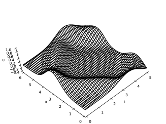
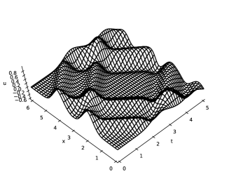
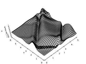
Figure 1. $U_{k}^{(n)}$ in Case 1 (upper left), Case 2 (upper right) and Case 3 (lower)

The energy conservation for the solutions are confirmed from Figure 2.

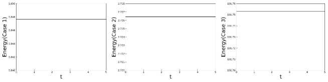
Figure 2. The conservation of the energy $J_{\mathrm{d}}(\mbox{\boldmath$U$}^{(n+1)},\mbox{\boldmath$U$}^{(n)})$ for (3.37)

In Figure 3, we show a comparison with the case of Neumann boundary condition. When we studied the parabolic type problem such as the Cahn-Hilliard equation or the Allen-Cahn equation, the behavior of solution with dynamic boundary condition near boundary tends to the one with the Neumann boundary condition, due to the parabolic property. On the other hand, we can observe a distinct behavior in the case of hyperbolic problem.

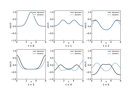
Figure 3. Comparison with Neumann boundary condition for the initial data $u(0,x)=e^{-(x-L/2)^{2}}$ and $\partial_{t}u(0,x)=0$ (Case 1)

Lastly, we also show the numerical simulation for the sine-Gordon equation:

(6.2) $$\left\{\begin{aligned} &\frac{\partial^{2}u}{\partial t^{2}}=\frac{\partial^{2}u}{\partial x^{2}}-\sin(u),&&(t,x)\in(0,6)\times(0,6),\\ &\frac{\partial^{2}u}{\partial t^{2}}(t,0)-\frac{\partial u}{\partial x}(t,0)=0,&&t\in(0,6),\\ &\frac{\partial^{2}u}{\partial t^{2}}(t,6)+\frac{\partial u}{\partial x}(t,6)=0,&&t\in(0,6).\end{aligned}\right.$$

As mentioned in Section 3, the corresponding difference scheme is given by (3.47).

The behavior of solutions are given in Figure 4. The simulation is demonstrated for the same initial conditions as the polynomial nonlinear case (6.1).

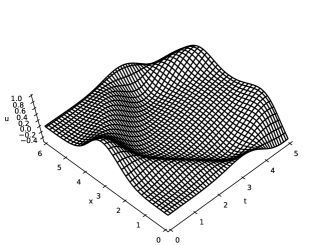
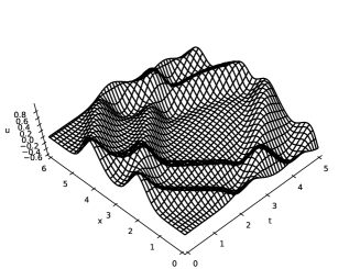
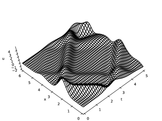
Figure 4. $U_{k}^{(n)}$ for (3.47) in Case 1 (upper left), Case 2 (upper right) and Case 3 (lower)

The energy conservation for the solutions are confirmed from Figure 5.

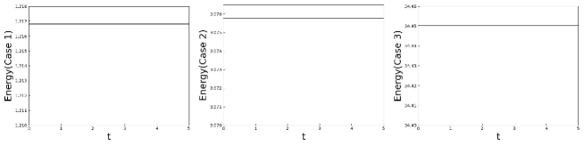
Figure 5. The conservation of the energy $J_{\mathrm{d}}(\mbox{\boldmath$U$}^{(n+1)},\mbox{\boldmath$U$}^{(n)})$ for (3.47)

References

- [1] L. Cherfils and M. Petcu, A numerical analysis of the Cahn–Hilliard equation with non-permeable walls, Numer. Math., 128 (2014), 517–549.
- [2] T. Fukao, S. Yoshikawa, S. Wada, Structure-preserving finite difference schemes for the Cahn-Hilliard equation with dynamic boundary conditions in the one-dimensional case, Commun. Pure. Appl. Anal., 16 (2017)
- [3] D. Furihata and T. Matsuo, Discrete Variational Derivative Method, Numerical Analysis and Scientific Computing Series, CRC Press/Taylor & Francis, 2010.
- [4] D. Furihata, Finite-difference schemes for nonlinear wave equation that inherit energy conservation property, J. Comput. Appl. Math., 134 (2001).
- [5] B. Kovács, C. Lubich, Stability and convergence of time discretizations of quasi-linear evolution equations of Kato type, Numer. Math., 138 (2018), 365–388.
- [6] B. Kovács and C. Lubich, Numerical analysis of parabolic problems with dynamic boundary conditions, IMA J. Numer. Anal., 37 (2017), 1–39.
- [7] H. Israel, A. Miranville and M. Petcu, Numerical analysis fo a Cahn-Hilliard type equation with dynamic boundary conditions, Recerche Mat., 64 (2015), 25-50.
- [8] T. Meurer, A. Kugi, Tracking control design for a wave equation with dynamic boundary conditions modeling a piezoelectric stack actuator, Int. J. Robust Nonlin., 21 (2011), 542-562.
- [9] A. Miranville, The Cahn–Hilliard equation and some of its variants, AIMS Math., 2(2017), 479-544.
- [10] F. Nabet, Convergence of a finite-volume scheme for the Cahn-Hilliard equation with dynamic boundary conditions, IMA J. Numer. Anal., 36 (2016), 1898-1942.
- [11] F. Nabet, An error estimate for a finite-volume scheme for the Cahn-Hilliard equation with dynamic boundary conditions, preprint hal-01273945 (2018), 1-32.
- [12] M. Okumura and D. Furihata, A structure-preserving scheme for the Allen-Cahn equation with a dynamic boundary condition, Discrete Contin. Dyn. Syst., 40(2020), 4927-4960.
- [13] M. Okumura, T. Fukao, D. Furihata, S. Yoshikawa, A second-order accurate structure-preserving scheme for the Cahn-Hilliard equation with a dynamic boundary condition, arXiv:2007.08355.
- [14] K. Yano, S. Yoshikawa, Structure-preserving finite difference schemes for a semilinear thermoelastic system with second order time derivative, Japan J. Ind. Appl. Math., 35(2018), 1213-1244.
- [15] S. Yoshikawa,Energy method for structure-preserving finite difference schemes and some properties of difference quotient,J. Comput. Appl. Math., 311 (2017), 394–413.
- [16] S. Yoshikawa, Remarks on energy methods for structure-preserving finite difference schemes -Small date global existence and unconditional error estimate, Appl. Math. Comput., 341 (2019), 80–92.
- [17] S. Yoshikawa, S. Kawashima, Global existence for a semi-discrete scheme of some quasilinear hyperbolic balance laws, J. Math. Appl. Anal., 498 (2021), 124929.