$q$-generalized Tsallis thermostatistics in Unruh effect for mixed fields

Abstract

It was shown that the particle distribution detected by a uniformly accelerated observer in the inertial vacuum (Unruh effect) deviates from the pure Planckian spectrum when considering the superposition of fields with different masses. Here we elaborate on the statistical origin of this phenomenon. In a suitable regime, we provide an effective description of the emergent distribution in terms of the nonextensive $q$-generalized statistics based on Tsallis entropy. This picture allows us to establish a nontrivial relation between the $q$-entropic index and the characteristic mixing parameters $\sin\theta$ and $\Delta m$. In particular, we infer that $q<1$, indicating the superadditive feature of Tsallis entropy in this framework. We discuss our result in connection with the entangled condensate structure acquired by the quantum vacuum for mixed fields.

I Introduction

The phenomenon of quantum mixing, i.e. the superposition of particle states with different masses, is among the most challenging topics in Particle Physics. In the Standard Model, it appears in the quark sector through Kobayashi-Maskawa matrix KM , a three-family generalization of Cabibbo mixing matrix between $d$ and $s$ quarks Cabi . On the other hand, convincing evidences of flavor mixing and oscillations in the neutrino sector have been provided in recent years by Super-Kamiokande SKK and SNO experiments SNO , confirming Pontecorvo’s pioneering idea Pont and opening a window into physics beyond the Standard Model.

Recently, the relevance of mixing transformations has prompted their study from a more fundamental field-theoretical (QFT) perspective. QFT effects on flavor mixing have been analyzed both for Dirac fermions BV95 and bosons BlasCap . This has uncovered the limits of the original quantum mechanical approach by pointing out the orthogonality between the vacuum for fields with definite flavor and that for fields with definite mass, the former becoming a condensate of particle-antiparticle pairs. The properties of flavor vacuum have been further explored in Cabo , where it has been shown that the Fock space for flavor fields cannot be obtained by the direct product of the Fock spaces for massive fields. Therefore, the nontrivial nature of mixing appears as a genuine QFT feature boiling down to the nonfactorizability of the flavor states in terms of those with definite mass, including the vacuum state (flavor vacuum).

All of the above studies have been developed in Minkowski spacetime. The QFT approach to mixing has been extended to Rindler (uniformly accelerated) metric in Luciano ; NonTN and to curved background in Quaranta . In particular, in Luciano ; NonTN it has been found that the vacuum condensate detected by the Rindler observer due to Unruh effect Unruh deviates from the Planckian density profile in the presence of mixed fields, the departure being dependent on the mass difference and the mixing angle. Such a result has been originally interpreted as a breakdown of the thermality of Unruh radiation for mixed fields. In passing, we mention that unconventional behaviors of Unruh effect are not entirely unusual in the literature, see for instance Dop ; Hammad ; deformed1 ; deformedPet and possible implications for particle decays Decay1 ; Decay2 ; Decay3 .

In its traditional form, the particle number spectrum of Unruh condensate follows the rules of Boltzmann-Gibbs statistics. However, in Tsallis1 ; Tsallis2 ; Tsallis3 ; Tsallis4 it has been argued that systems exhibiting long-range interactions and/or spacetime entanglement, either on quantum or classical grounds, require a generalization of Boltzmann-Gibbs theory to the so called nonextensive Tsallis $q$-thermostatistics. This occurs through a suitable (nonadditive) redefinition of the entropy, which still recovers Boltzmann-Gibbs formula in the $q=1$ limit. The $q$-generalized statistical mechanics proposed by Tsallis has provided encouraging results in describing a broad class of complex systems, such as self-gravitating stellar systems App1 ; App3 , black holes Tsallis3 , the cosmic background radiation App7 ; App8 , low-dimensional dissipative systems Tsallis4 , solar neutrinos App11 , polymer chains Polch and modified cosmological models App13 ; App14 , among others. Furthermore, it has paved the way for an intensive study of alternative statistical models within the framework of information theory Ren .

Starting from the above premises, in this work we feature the entangled condensate structure of the vacuum for mixed fields in the language of nonextensive Tsallis statistics. We consider Unruh effect as a specific playground. In this context, it is shown that the modified Unruh distribution for mixed fields can be described by an appropriately $q-$generalized distribution based on Tsallis entropy. This allows us to establish an effective connection between the nonextensive $q$-entropic index and the characteristic mixing parameters $\sin\theta$ and $\Delta m$ in a suitable approximation. We find that $q<1$, which corresponds to a superadditive Tsallis entropy. To make our analysis as transparent as possible, we deal with a simplified model involving only two scalar fields. The case of fermion mixing will be shortly addressed at the end with similar results.

The remainder of this paper is structured as follows: in Sec. II we analyze the canonical quantization of a massive scalar field for the Rindler observer using the Bogoliubov transformation method. This leads us to derive the Unruh effect in a natural way. Section III contains the study of the QFT formalism of flavor mixing in Rindler spacetime. Exploiting these tools, in Sec. IV we introduce the basics of nonextensive Tsallis thermostatistics and investigate the connection with field mixing at the level of Unruh vacuum condensate. We discuss our result in relation with the complex condensate structure acquired by the quantum vacuum for mixed fields. Conclusions and outlook are summarized in Sec. V. The work ends with an Appendix devoted to review the theory of field mixing in Minkowski background.

Throughout all the manuscript, we adopt the mostly negative signature for the $4$-dimensional metric and natural units $\hslash=c=k_{\mathrm{B}}=1$. Furthermore, we use the notation

$$x=\{t,\textbf{x}\},\qquad{\bf{x}}=\{x^{1},\vec{x}\},\qquad\vec{x}=\{x^{2},x^{3}\}\,,$$ (1)

for $4$-, $3$- and $2$-vectors, respectively.

II QFT in Rindler spacetime and Unruh effect

In this Section we briefly review the quantization of a massive scalar field for a uniformly accelerated (Rindler) observer. Without loss of generality, we assume the acceleration to be along the $x^{1}$-axis. In this setting, it is useful to introduce the new coordinates $-\infty<\eta,\xi<\infty$, such that $t=\xi\sinh\eta$, $x^{1}=\xi\cosh\eta$, while leaving $\vec{x}$ unchanged. In terms of these coordinates, Minkowski metric takes the form

$$ds^{2}={(dt)}^{2}-{(dx^{1})}^{2}-\sum_{j=2}^{3}{(dx^{j})}^{2}\underset{\tiny{Rindler\;coord.}}{\longrightarrow}ds^{2}=\xi^{2}d\eta^{2}-d\xi^{2}-\sum_{j=2}^{3}{(dx^{j})}^{2}\,,$$ (1)

which admits $B=\partial/\partial{\eta}$ as a time-like Killing vector. Henceforth, we refer to the coordinates $\{t,x^{1}\}$ and $\{\eta,\xi\}$ as Minkowski and Rindler coordinates, respectively. Accordingly, the metric (1) shall be named Rindler metric.

Let us now consider the world-line of fixed spatial coordinates, i.e.

$$\xi(\tau)=a^{-1}=\mathrm{const}\,,\quad\vec{x}(\tau)=\mathrm{const},$$ (2)

where $\tau$ is the proper time measured along the line. Substitution of Eq. (2) into the metric (1) yields $\eta(\tau)=a\tau$, i.e., the proper time $\tau$ for an observer moving along the line (2) is the same as the Rindler time $\eta$, up to the scale factor $a$.

In Minkowski coordinates Eq. (2) becomes

$$t(\tau)=a^{-1}\sinh a\tau,\quad x^{1}(\tau)=a^{-1}\cosh a\tau,\quad\vec{x}(\tau)=\mathrm{const}\,,$$ (3)

which is an hyperbola with asymptotes $t=\pm x^{1}$ in the $(t,x^{1})$ plane. In special relativity, it is well known that the hyperbolic motion generalizes the concept of Newtonian uniformly accelerated motion, with $|a|$ being the magnitude of the proper acceleration Mukhanov . In particular, for $a>0$ the observer moves along the branch of hyperbola in the right wedge $R_{+}=\{x|x^{1}>|t|\}$, while for $a<0$ the motion occurs in the left wedge $R_{-}=\{x|x^{1}<-|t|\}$ (see Fig. 1). This reveals the peculiar features of the causal structure of Rindler spacetime: since a uniformly accelerated observer in $R_{+}$ cannot receive (send) any signal from (to) the future (past) wedge $t>|x^{1}|$ $(t<-|x^{1}|)$, the asymptote $t=|x^{1}|$ ($t=-|x^{1}|$) appears to him as a future (past) event horizon. Notice that the time ordering of the two horizons is reversed in $R_{-}$, since the Killing vector $B$ is past oriented in this wedge. Accordingly, a Rindler observer in $R_{+}$ turns out to be causally separated from $R_{-}$, and vice-versa.

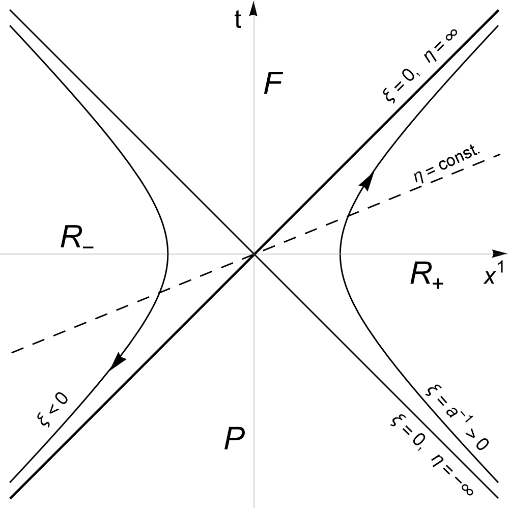
Figure 1: Causal structure of Rindler metric in $1+1$ dimensions. We are assuming that Rindler observer accelerates along the $x^{1}$-axis, while the transverse dimensions $x^{2},x^{3}$ are kept constant during the motion. The arrow indicates the direction of motion.

Bearing in mind the causal structure of the metric (1), let us deal with the quantization of a charged scalar field $\phi(x)$ of mass $m$ for the Rindler observer. In Rindler coordinates, the Klein-Gordon equation reads

$$\bigg{\{}{\bigg{(}\frac{\partial}{\partial t}\bigg{)}}^{2}-\sum_{j=1}^{3}{\bigg{(}\frac{\partial}{\partial x^{j}}\bigg{)}}^{2}+m^{2}\bigg{\}}\hskip 0.28453pt\,\phi(x)=0\underset{Rindler\;coord.}{\longrightarrow}\bigg{\{}\frac{1}{\xi^{2}}\frac{\partial^{2}}{\partial\eta^{2}}-\frac{\partial^{2}}{\partial\xi^{2}}-\frac{1}{\xi}\frac{\partial}{\partial\xi}-\sum_{j=2}^{3}{\bigg{(}\frac{\partial}{\partial x^{j}}\bigg{)}}^{2}+m^{2}\bigg{\}}\hskip 0.28453pt\,\phi(x)=0\,,$$ (4)

which has the modes

$$u_{\kappa}^{\,(\sigma)}(x)=\frac{\theta(\sigma\xi)}{2\pi\Omega}\frac{1}{\Gamma(i\Omega)^{2}\sqrt{\sinh(\pi\Omega)}}\hskip 0.56905ptK_{i\Omega}(\mu_{k}\xi)\hskip 0.28453pte^{i\left(\vec{k}\cdot\vec{x}-\sigma\Omega\eta\right)}\,,$$ (5)

as solutions of frequency $\Omega>0$ with respect to the time coordinate $\eta$. Following Takagi , here we have introduced the shorthand notation $\kappa\equiv(\Omega,\vec{k})$. The Heaviside step function $\theta(\sigma\xi)$ restricts the support of $u_{\kappa}^{\,(\sigma)}$ to only one of the two Rindler wedges. Specifically, $\sigma=+$ refers to the right wedge $R_{+}$, while $\sigma=-$ to the left wedge. The function $\Gamma(i\Omega)$ is the usual Euler’s gamma, while $K_{i\Omega}(\mu_{k}\xi)$ denotes the modified Bessel function of second kind. The reduced Minkowski frequency is given by $\mu_{k}={(m^{2}+|\vec{k}|^{2})}^{1/2}$.

It is easy to verify that the Rindler modes (5) form a complete and orthonormal set with respect to the Klein-Gordon product in Rindler coordinates. This allows us to take the following expansion for the scalar field Takagi

$$\phi(x)=\sum_{\sigma,\hskip 1.13809pt\Omega}\,\int d^{2}k\,\Big{\{}{b^{\,(\sigma)}_{\kappa}}\,u_{\kappa}^{\,(\sigma)}(x)+{\bar{b}^{\,(\sigma)\dagger}_{\kappa}}\,u_{\kappa}^{\,(\sigma)*}(x)\Big{\}},$$ (6)

where $\sum_{\sigma,\hskip 1.13809pt\Omega}$ stands for $\sum_{\sigma=\pm}\int_{0}^{\infty}d\Omega\hskip 0.56905pt$. The ladder operators ${b^{\,(\sigma)}_{\kappa}}$ (${\bar{b}^{\,(\sigma)}_{\kappa}}$) are assumed to be canonical. They act as annihilators of Rindler particles (antiparticles) of frequency $\Omega$ and transverse momentum $\vec{k}$ in the wedge $R_{\sigma}$. Rindler vacuum $|0_{\mathrm{R}}\rangle$ is defined by $b_{\kappa}^{\,(\sigma)}|0_{\mathrm{R}}\rangle=\bar{b}_{\kappa}^{\,(\sigma)}|0_{\mathrm{R}}\rangle=0$, $\forall\sigma,\kappa\,$. On the other hand, ${b^{\,(\sigma)\dagger}_{\kappa}}$ (${\bar{b}^{\,(\sigma)\dagger}_{\kappa}}$) creates a Rindler particle (antiparticle) with the same quantum numbers as defined above.

We now focus on the relation between the quantization (6) and the Minkowski plane-wave expansion

$$\phi(x)=\int d^{3}{k}\,\Big{\{}a_{\textbf{k}}\,U_{\textbf{k}}(x)+{\bar{a}_{\textbf{k}}}^{\dagger}\,U_{\textbf{k}}^{\hskip 0.28453pt*}(x)\Big{\}},$$ (7)

where $U_{\bf{k}}(x)={[{2\omega_{{\bf{k}}}{(2\pi)}^{3}}]}^{-1/2}e^{i\left({\bf{k}}\cdot{\bf{x}}-\omega_{{\bf{k}}}t\right)}$ are the plane-waves of frequency $\omega_{\textbf{k}}=({m^{2}+|\textbf{k}|^{2}})^{1/2}$. Here, $a_{{\bf{k}}}$ ($\bar{a}_{{\bf{k}}}$) denote the canonical annihilators of Minkowski particles (antiparticles) with momentum ${\bf{k}}$ and frequency $\omega_{{\bf{k}}}$, such that $a_{\bf{k}}|0_{\mathrm{M}}\rangle=\bar{a}_{\bf{k}}|0_{\mathrm{M}}\rangle=0$, $\forall{\bf{k}}$, where $|0_{\mathrm{M}}\rangle$ is the Minkowski vacuum. As before, the rôle of creation operators is played by the adjoint $a^{\dagger}_{\bf{k}}$ ($\bar{a}^{\dagger}_{\bf{k}}$). Since this formalism holds for the set of inertial observers in Minkowski spacetime, in what follows we indifferently refer to the expansion (7) as either Minkowski or inertial field quantization.

To derive the Bogoliubov transformation between the two field representations introduced above, we compare the expansions (6) and (7) on a space-like hypersurface $\Sigma$ which lies in the Rindler manifold $R_{\pm}$. By multiplying both sides by the Rindler mode $u^{(\sigma)}_{\kappa}$, we obtain Takagi

$$b_{\kappa}^{\,(\sigma)}=\int d^{3}k^{\prime}\left\{a_{\textbf{k}^{\prime}}\hskip 0.28453pt(u^{(\sigma)}_{\kappa},U_{\textbf{k}^{\prime}})\,+\,\bar{a}^{\dagger}_{\textbf{k}^{\prime}}\hskip 0.28453pt(u^{(\sigma)}_{\kappa},U^{*}_{\textbf{k}^{\prime}})\right\}\,.$$ (8)

The explicit expressions of the Bogoliubov coefficients $(u^{(\sigma)}_{\kappa},U_{\textbf{k}^{\prime}})$ and $(u^{(\sigma)}_{\kappa},U^{*}_{\textbf{k}^{\prime}})$ are rather awkward to exhibit. They are given in Takagi . However, Eq. (8) can be cast in a more transparent form by introducing the following superposition of $a_{\textbf{k}}$-operators

$$d_{\kappa}^{\,(\sigma)}=\int dk_{1}\,\frac{1}{\sqrt{2\pi\omega_{\bf{k}}}}\,{\bigg{(}\frac{\omega_{{\bf{k}}}+k_{1}}{\omega_{{\bf{k}}}-k_{1}}\bigg{)}}^{i\sigma\Omega/2}\,a_{{\bf{k}}},$$ (9)

(similarly, the definition of $\bar{d}_{\kappa}^{\,(\sigma)}$ is obtained by replacing $a_{{\bf{k}}}$ with $\bar{a}_{{\bf{k}}}$). In Takagi , it has been shown that these new operators still obey the canonical commutator. Furthermore, they share a common vacuum with the $a_{\textbf{k}}$’s, since they are linear combinations of these annihilators only. In other terms, the $d$-operators provide an alternative representation for the scalar field, which is unitarily equivalent to the plane-wave quantization from the perspective of inertial observers. This has been discussed in more detail in Luciano .

In terms of the operators (9), Eq. (8) can be rewritten as

$$b_{\kappa}^{\,(\sigma)}=\sqrt{1+N_{\mathrm{BE}}(\Omega)}\hskip 0.28453ptd_{\kappa}^{\,(\sigma)}\,+\,\sqrt{N_{\mathrm{BE}}(\Omega)}\hskip 0.28453pt\bar{d}_{\tilde{\kappa}}^{\,(-\sigma)\,\dagger}\,,$$ (10)

where $\tilde{\kappa}\equiv(\Omega,-\vec{k})$ and

$$N_{\mathrm{BE}}(\Omega)=\frac{1}{e^{2\pi\Omega}-1}\,.$$ (11)

is the Bose-Einstein distribution function.

Next, by resorting to Eqs. (9) and (10), we can evaluate the expected number spectrum of Rindler particles in the Minkowski vacuum, obtaining

$$\langle 0_{\mathrm{M}}|b_{\kappa^{\prime}}^{\,(\sigma^{\prime})\dagger}\hskip 0.56905ptb_{\kappa}^{\,(\sigma)}|0_{\mathrm{M}}\rangle=N_{\mathrm{BE}}(\Omega)\hskip 0.56905pt\delta_{\sigma\sigma^{\prime}}\hskip 0.56905pt\delta^{3}(\kappa-\kappa^{\prime})\,,$$ (12)

(similarly for $\bar{b}_{\kappa}^{\,(\sigma)}$). Since the proper energy of quanta detected by an observer moving with uniform acceleration $a$ is

$$E=a\Omega\,,$$ (13)

it is more appropriate to rewrite the distribution (11) in the form

$$N_{\mathrm{BE}}(\Omega)=\frac{1}{e^{E/T_{\mathrm{U}}}-1}\,,$$ (14)

where $T_{\mathrm{U}}=a/(2\pi)$ is the Unruh temperature Unruh . Thus, we recover the well-known Unruh result that Minkowski vacuum appears as a Bose-Einstein thermal distribution of Rindler particles, with temperature $T_{\mathrm{U}}$ being proportional to the magnitude of the proper acceleration Unruh .

As discussed in Takagi , the inherent properties of the condensate (12) can be explored in depth by expressing the Minkowski vacuum $|0_{\mathrm{M}}\rangle$ in terms of the Rindler one $|0_{\mathrm{R}}\rangle$. In so doing, we infer that the inertial vacuum acquires the structure of a coherent state of pairwise-correlated Rindler particles. Specifically, an excitation in the positive wedge $R_{+}$ is correlated to an excitation of opposite spatial momentum in the negative region $R_{+}$, and vice-versa. Since the two wedges are causally disconnected, this turns out to be an EPR-like correlation between space-like separated quanta.

The spectrum (12) diverges for any fixed $\kappa=\kappa^{\prime}$. This is due to the fact that the creation operators $a_{{\bf{k}}}^{\dagger}$, $b_{\kappa}^{\dagger}$ (and the corresponding operators for antiparticles) do not produce normalizable states when applied on the respective vacua. To avoid conceptual difficulties we shall otherwise encounter later, we introduce the following set of functions Hawk1995

$$f_{nl}(k)=\chi_{n}(k)\exp^{-2\pi ilk/\varepsilon}\,,$$ (15)

$$\chi_{n}(k)=\left\{\begin{array}[]{rcl}&&\varepsilon^{-1/2}\,\,\,\,\,\,\,\,\,\mathrm{for}\left(n-\frac{1}{2}\right)\varepsilon<k<\left(n+\frac{1}{2}\right)\varepsilon\\[8.53581pt] &&0\,\,\,\,\,\,\,\,\,\,\,\,\,\,\,\,\,\,\,\,\mathrm{otherwise}\end{array}\right.\,,$$ (16)

where $\varepsilon$ is a positive constant of dimension of inverse length. By exploiting the completeness and orthonormality of this set Takagi , we define the Minkowski wave packet by

$$U_{nl\vec{k}}(x)=\int dk_{1}f_{nl}(k_{1})U_{{\bf{k}}}(x)\,,$$ (17)

where $n$ and $l$ run over all the integers.

On the other hand, to form the Rindler wave packet, we restrict the subscript $n$ of $\{f_{nl}\}$ to positive integers. Notice that this does not affect the orthonormality nor the completeness of the set (15), provided that the argument $k$ is now replaced by the Rindler frequency $\Omega$ and $\varepsilon$ is assumed to be dimensionless. We then define

$$u_{nl\vec{k}}(x)=\int_{0}^{\infty}d\Omega f_{nl}(\Omega)u^{(\sigma)}_{\kappa}(x)\,.$$ (18)

Two comments are in order here: first, the wave packets (17) and (18) satisfy a box-like normalization and are complete, due to the definition (15) of the smearing function. Furthermore, in the above construction we have left the reduced momentum $\vec{k}$ untouched, as it does not enter the Bose-Einstein distribution function (14) explicitly. More properly, we should extend the wave packet formalism to this quantum number as well, resulting in a new pair of subscripts in place of each component of $\vec{k}$. However, since this procedure would burden the notation without providing any conceptual advantage, we continue to use the symbol $\vec{k}$, taking care of this aspect.

We can now repeat the computation of the number spectrum of Rindler particles in the Minkowski vacuum. By choosing the parameter $\varepsilon$ in the definition of $f_{nl}(k_{1})$ much less than the reduced Minkowski frequency $\mu_{k}$ and the $\varepsilon$ in $f_{nl}(\Omega)$ much less than unity, we are led to Takagi

$$\langle 0_{\mathrm{M}}|\hskip 0.56905ptb_{n^{\prime}l^{\prime}\vec{k}^{\prime}}^{\,(\sigma^{\prime})\dagger}\hskip 0.28453ptb_{nl\vec{k}}^{\,(\sigma)}\hskip 0.56905pt|0_{\mathrm{M}}\rangle=N_{\mathrm{BE}}({\Omega_{n}})\delta_{\sigma\sigma^{\prime}}\delta_{nn^{\prime}}\delta_{ll^{\prime}}\delta_{\vec{k}\vec{k^{\prime}}}\,,$$ (19)

where $\Omega_{n}=n\varepsilon$. Of course, for fixed values of $\sigma=\sigma^{\prime},n=n^{\prime},l=l^{\prime},m=m^{\prime}$ and $\vec{k}=\vec{k}^{\prime}$, this gives

$$\mathcal{N}(\Omega_{n})\equiv\langle 0_{\mathrm{M}}|\hskip 0.56905ptb_{nl\vec{k}}^{\,(\sigma)\dagger}\hskip 0.28453ptb_{nl\vec{k}}^{\,(\sigma)}\hskip 0.56905pt|0_{\mathrm{M}}\rangle=N_{\mathrm{BE}}({\Omega_{n}})\,,$$ (20)

As expected, the use of properly normalizable wave packets results into a regularization of the Unruh spectrum (12). In the next Section, we shall see how the distribution (20) is modified when dealing with the superposition of fields with different masses.

III QFT of flavor mixing in Rindler spacetime

The QFT treatment of flavor mixing, originally developed for Dirac neutrinos in Minkowski background BV95 and later extended to mesons, such as the $K^{0}-\bar{K}^{0}$, $B^{0}-\bar{B}^{0}$ and $\eta-\eta^{\prime}$ systems BlasCap ; Ji , has revealed a series of nontrivial features that are totally missed by quantum mechanics. These aspects are reviewed in the Appendix, with particular emphasis on the issue of the unitary inequivalence between the Fock space for fields with definite flavor and the Fock space for fields with definite mass. Following Luciano , here we generalize the quantization of mixed fields to the Rindler metric. We consider the mixing transformations in a simplified two-flavor model with charged scalar fields. Denoting by $\chi=A,B$ ($i=1,2$) the flavor (mass) label, these transformations read

$$\phi_{A}(x) = \phi_{1}(x)\,\cos\theta+\phi_{2}(x)\,\sin\theta\,,$$ (21)

$$\phi_{B}(x) = -\phi_{1}(x)\,\sin\theta+\phi_{2}(x)\,\cos\theta\,,$$ (22)

where $\theta$ is the mixing angle and $\phi_{i}$ ($i=1,2$) are two free charged scalar fields of masses $m_{i}$, such that $m_{2}\neq m_{1}$. For definiteness, we set $m_{2}>m_{1}$. Let $\pi_{i}=\partial_{t}\phi_{i}^{\dagger}$ be the conjugate momenta.

In the canonical quantization formalism, it is known that

$$\qquad\big{[}\phi_{i}(x),\,\pi_{j}(x^{\prime})\big{]}_{t=t^{\prime}}=\big{[}\phi^{\dagger}_{i}(x),\,\pi^{\dagger}_{j}(x^{\prime})\big{]}_{t=t^{\prime}}=i\,\delta^{3}(x-x^{\prime})\,\delta_{ij}\,,\qquad i,j=1,2\,,$$ (23)

with all other equal-time commutators vanishing. In the Appendix we discuss the algebraic structure of Eqs. (21) and (22), showing that each of them appears as a rotation combined with a Bogoliubov transformation when seen at level of ladder operators. Notice that this peculiar structure, which is absent in quantum mechanics, arises from the necessity to take account of the antiparticle degrees of freedom intrinsically built in QFT. As a result, the vacuum state for flavor fields becomes a condensate of massive particle-antiparticle pairs (see Eq. (60)).

To find out how the phenomenon of mixing appears to the Rindler observer, we retrace the same steps leading to Eq. (6) and consider the following free field-like expansions for mixed fields Luciano

$$\phi_{\ell}(x)=\sum_{\sigma,\hskip 1.13809pt\Omega}\,\int d^{2}k\,\Big{\{}{b^{\,(\sigma)}_{\kappa,\ell}}(\eta)\,u_{\kappa,j}^{\,(\sigma)}(x)+{\bar{b}^{\,(\sigma)\dagger}_{\kappa,\ell}}(\eta)\,u_{\kappa,j}^{\,(\sigma)*}(x)\Big{\}},\quad(\ell,j)=\left\{(A,1),(B,2)\right\},$$ (24)

where we have used the shorthand notation $b^{\,(\sigma)}_{\kappa,\ell}(\eta)\equiv b^{\,(\sigma)}_{\kappa,\ell}(\theta,\eta)$ for the ladder operators (similarly for $\bar{b}^{\,(\sigma)}_{\kappa,\ell}(\eta)$). By comparison with Eq. (54), it is clear that these operators provide the Rindler counterpart of Minkowski flavor annihilators given in Eq. (55). It is a matter of calculations to show that they obey the (equal-time) canonical commutators.

As remarked above, the mixing relations at level of ladder operators hide a Bogoliubov transformation between the flavor and mass bases. At the same time, the field quantizations for Minkowski and Rindler observers are connected to each other by the Bogoliubov transformation (10) responsible for the thermal Unruh effect. Overall, we expect that the Rindler annihilators in the flavor representation are related to the corresponding Minkowski operators in the mass basis by a combination of these two Bogoliubov transformations. To analyze such an interplay, we compare the expansions (24) and (54). By using Eqs. (21)-(22) and the transformation (55), after some tedious but straightforward calculations, we obtain Luciano

$$b_{\kappa,A}^{\,(\sigma)} = \sqrt{1+N_{\mathrm{BE}}(\Omega)}\,\,\Big{[}\cos\theta\,d_{\kappa,1}^{\,(\sigma)}\,+\,\sin\theta\sum_{\hskip 1.70717pt\sigma^{\prime},\hskip 0.28453pt\Omega^{\prime}}\Big{(}d_{(\Omega^{\prime},\vec{k}),2}^{\,(\sigma^{\prime})}\,\;{\cal A}_{(\Omega,\Omega^{\prime}),\,\vec{k}}^{(\sigma,\sigma^{\prime})}\,+\,\bar{d}_{(\Omega^{\prime},-\vec{k}),2}^{\,(\sigma^{\prime})\dagger}\,\;{\cal B}_{(\Omega,\Omega^{\prime}),\,\vec{k}}^{(\sigma,\sigma^{\prime})}\,\Big{)}\Big{]}$$

$$+ \,\sqrt{N_{\mathrm{BE}}(\Omega)}\,\,\Big{[}\cos\theta\,\bar{d}_{\tilde{\kappa},1}^{\,(-\sigma)\dagger}\,+\,\sin\theta\sum_{\hskip 1.70717pt\sigma^{\prime},\hskip 0.28453pt\Omega^{\prime}}\Big{(}\bar{d}_{(\Omega^{\prime},-\vec{k}),2}^{(-\sigma^{\prime})\dagger}\,\;{\cal A}_{(\Omega,\Omega^{\prime}),\,\vec{k}}^{(\sigma,\sigma^{\prime})}\,+\,d_{(\Omega^{\prime},\vec{k}),2}^{(-\sigma^{\prime})}\,\;{\cal B}_{(\Omega,\Omega^{\prime}),\,\vec{k}}^{(\sigma,\sigma^{\prime})}\,\Big{)}\Big{]},$$

where we have omitted for simplicity the time-dependence of $b_{\kappa,A}^{\,(\sigma)}$ (a similar expression hold true for $b_{\kappa,B}^{\,(\sigma)}$ as well). We stress that the $d$-operators are an equivalent way of rewriting the standard Minkowski annihilators appearing in Eq. (7) (see Eq. (9)). From the above relation, we can clearly distinguish the action of the thermal Bogoliubov transformation (encoded by the coefficients ${(1+N_{\mathrm{BE}})^{1/2}}$ and ${N^{1/2}_{\mathrm{BE}}}$) from the action of the mixing Bogoliubov transformation (which appears through the coefficients ${\cal A}_{(\Omega,\Omega^{\prime}),\,\vec{k}}^{(\sigma,\sigma^{\prime})}$ and ${\cal B}_{(\Omega,\Omega^{\prime}),\,\vec{k}}^{(\sigma,\sigma^{\prime})}$). The Bogoliubov coefficients related to mixing are given by Luciano

$${\cal A}_{(\Omega,\Omega^{\prime}),\,\vec{k}}^{(\sigma,\sigma^{\prime})}=\int^{+\infty}_{-\infty}\frac{dk_{1}}{4\pi}\left(\frac{1}{\omega_{{\bf{k}},1}}+\frac{1}{\omega_{{\bf{k}},2}}\right){\left(\frac{\omega_{{\bf{k}},1}+k_{1}}{\omega_{{\bf{k}},1}-k_{1}}\right)}^{i\sigma\Omega/2}{\left(\frac{\omega_{{\bf{k}},2}+k_{1}}{\omega_{{\bf{k}},2}-k_{1}}\right)}^{-i\sigma^{\prime}\Omega^{\prime}/2}e^{i(\omega_{{\bf{k}},1}-\,\omega_{{\bf{k}},2})t}\,,$$ (26)

$${\cal B}_{(\Omega,\Omega^{\prime}),\,\vec{k}}^{(\sigma,\sigma^{\prime})}=\int^{+\infty}_{-\infty}\frac{dk_{1}}{4\pi}\left(\frac{1}{\omega_{{\bf{k}},2}}-\frac{1}{\omega_{{\bf{k}},1}}\right){\left(\frac{\omega_{{\bf{k}},1}+k_{1}}{\omega_{{\bf{k}},1}-k_{1}}\right)}^{i\sigma\Omega/2}{\left(\frac{\omega_{{\bf{k}},2}+k_{1}}{\omega_{{\bf{k}},2}-k_{1}}\right)}^{-i\sigma^{\prime}\Omega^{\prime}/2}e^{i(\omega_{{\bf{k}},1}+\,\omega_{{\bf{k}},2})t}\,.$$ (27)

Despite the nontrivial structure of ${\cal A}_{(\Omega,\Omega^{\prime}),\,\vec{k}}^{(\sigma,\sigma^{\prime})}$ and ${\cal B}_{(\Omega,\Omega^{\prime}),\,\vec{k}}^{(\sigma,\sigma^{\prime})}$, interesting implications of Eq. (III) can still be derived for $t=\eta=0$ and in the reasonable approximation of small difference between the masses of the two fields, i.e. $|\Delta m^{2}|/{m_{1}^{2}}=|m_{2}^{2}-m_{1}^{2}|/m_{1}^{2}\ll 1$. Indeed, if we evaluate the number spectrum of mixed particles detected by the Rindler observer in the inertial vacuum, we get to the leading order Luciano

$$\langle 0_{\mathrm{M}}|\,b_{\kappa,\chi}^{\,(\sigma)\dagger}(0)\,b_{\kappa^{\prime},\chi}^{\,(\sigma)}(0)\,|0_{\mathrm{M}}\rangle\,=\,N_{\mathrm{BE}}(\Omega)\,\delta^{3}(\kappa-\kappa^{\prime})-\,\frac{|\Delta m^{2}|}{8\,\mu_{k,1}^{\hskip 0.28453pt2}}\sin^{2}\theta\,\frac{\sigma\,(\Omega^{\prime}+\Omega)\,G(\Omega,\Omega^{\prime})}{\sinh\left[\frac{\pi}{2}\,\sigma\,(\Omega^{\prime}+\Omega)\right]}\,\delta(\vec{k}-\vec{k}^{\prime})\,+\,\mathcal{O}\left(\frac{|\Delta m^{2}|}{\mu^{2}_{k,1}}\right)^{2}\,,$$ (28)

for $\chi=A,B$, where

$$G(\Omega,\Omega^{\prime})\equiv\sqrt{1+N_{\mathrm{BE}}(\Omega)}\,\sqrt{N_{\mathrm{BE}}(\Omega^{\prime})}\,+\,\sqrt{N_{\mathrm{BE}}(\Omega)}\,\sqrt{1+N_{\mathrm{BE}}(\Omega^{\prime})}\,.$$ (29)

Thus, the standard Bose-Einstein distribution of Unruh vacuum condensate (12) turns out to be spoilt in the presence of mixed fields. Notice that, for $\theta\rightarrow 0$, Eq. (28) recovers the usual result, as expected in the absence of mixing. Similar considerations hold true for $m_{1}\rightarrow m_{2}$ and in the relativistic limit $|\vec{k}|^{2}\gg m_{1}^{2}+m_{2}^{2}$, since the parameter ${|\Delta m^{2}|}/{\mu^{2}_{k,i}}$ becomes increasingly small.

As argued at the end of Sec. II, in order to avoid unphysical divergencies in the spectrum, it is convenient to revisit the above formalism by employing wave packets. With the aid of Eqs. (15)-(18), the density (20) of Rindler mixed particles with quantum numbers $\Omega_{n},l,\vec{k}$ then becomes

$$\mathcal{N}_{\theta,\Delta m}(\Omega_{n})\,\equiv\,\langle 0_{\mathrm{M}}|\hskip 0.56905ptb_{nl\vec{k}}^{\dagger}(0)\hskip 0.28453ptb_{nl\vec{k}}(0)|0_{\mathrm{M}}\rangle\,=\,N_{\mathrm{BE}}({\Omega_{n}})\,-\,\frac{|\Delta m^{2}|}{4\,\mu_{k,1}^{\hskip 0.28453pt2}}\sin^{2}\theta\,\frac{\Omega_{n}\,G(\Omega_{n},\Omega_{n})}{\sinh\left({\pi}\Omega_{n}\right)}\,+\,\mathcal{O}\left(\frac{|\Delta m^{2}|}{\mu^{2}_{k,1}}\right)^{2}\,,$$ (30)

where we have dropped the indices $\sigma$ and $\chi$ from $\langle 0_{\mathrm{M}}|\hskip 0.56905ptb_{nl\vec{k}}^{\dagger}(0)\hskip 0.28453ptb_{nl\vec{k}}(0)|0_{\mathrm{M}}\rangle$, since the r.h.s. of Eq (28) is in fact insensitive to them. By resorting to the definition (29) of $G(\Omega,\Omega)$, we are finally led to

$$\mathcal{N}_{\theta,\Delta m}(\Omega_{n})\,=\,N_{\mathrm{BE}}({\Omega_{n}})\,-\,\frac{|\Delta m^{2}|}{4\,\mu_{k,1}^{\hskip 0.28453pt2}}\sin^{2}\theta\,\Omega_{n}\operatorname{csch}^{2}(\pi\Omega_{n})\,+\,\mathcal{O}\left(\frac{|\Delta m^{2}|}{\mu^{2}_{k,1}}\right)^{2}\,,$$ (31)

where $\operatorname{csch}(x)=1/\sinh(x)$.

In Luciano the modified distribution (28) (or, equivalently, (31)) has been interpreted as being due to a breakdown of the thermality of Unruh radiation induced by field mixing. We further elaborate on the physical meaning of the result (31) in the next Section.

IV Flavor Mixing and q-generalized Tsallis statistics

In the standard Boltzmann-Gibbs thermodynamics, it is well known that entropy is an additive quantity, which means that, given two probabilistically independent systems $A$ and $B$ with entropies $S_{\mathrm{BG}}(A)$ and $S_{\mathrm{BG}}(B)$, respectively, the total entropy is simply $S_{\mathrm{BG}}(A+B)=S_{\mathrm{BG}}(A)+S_{\mathrm{BG}}(B)$. At the statistical level, the Boltzmann-Gibbs entropy of a system in an equilibrium macrostate can be expressed in terms of the corresponding microscopic configurations as

$$S_{\mathrm{BG}}=-\sum_{i=1}^{W}p_{i}\log p_{i}\,,$$ (32)

for a set of $W$ discrete microstates, where $\{p_{i}\}$ is the set of probability distribution with the condition $\sum_{i=1}^{W}p_{i}=1$. If probabilities are all equal, this takes the well-known form $S_{\mathrm{BG}}=\log W$. It is immediate to check that $S_{\mathrm{BG}}$ satisfies the additivity property as defined above.

Despite the wide range of applicability of the Boltzmann-Gibbs theory, for complex systems exhibiting long-range interactions and/or spacetime entanglement, it has been argued that the standard Boltzmann-Gibbs theory should be generalized to a nonextensive statistical mechanics based on the nonadditive Tsallis entropy Tsallis1 ; Tsallis2 ; Tsallis3 ; Tsallis4

$$S_{q}\,=\,\frac{1-\sum_{i=1}^{W}p_{i}^{q}}{q-1}\,=\,\sum_{i=1}^{W}p_{i}\log_{q}\frac{1}{p_{i}}\,,$$ (33)

with

$$\log_{q}z\equiv\frac{z^{1-q}-1}{1-q},\quad(\log_{1}z=\log z)\,.$$ (34)

Note that $S_{q}$ recovers Boltzmann-Gibbs entropy $S_{\mathrm{BG}}$ in the $q\rightarrow 1$ limit. Furthermore, by considering again two probabilistically independent systems such that $p_{ij}^{A+B}=p_{i}^{A}p_{j}^{B},\,\forall{(i,j)}$, the definition (33) leads to

$$S_{q}(A+B)=S_{q}(A)+S_{q}(B)+(1-q)S_{q}(A)S_{q}(B)\,,$$ (35)

indicating that $S_{q}$ is superadditive or subadditive, depending on whether $q<1$ or $q>1$. Thus, the dimensionless index $q\in\mathbb{R^{+}}$ quantifies the departure of Tsallis entropy from Boltzmann-Gibbs one. For this reason, it is named nonextensive Tsallis parameter. Paradigmatic examples of systems obeying the generalized statistics (33) are the strongly gravitating black holes Tsallis3 , albeit in recent years Tsallis thermostatistics has found applications in a variety of physical scenarios App1 ; App3 ; App7 ; App8 ; App11 ; App13 ; App14 .

Now, within an approximation called factorization approach, it has been shown that the Tsallis entropy (33) can be used to derive the following generalized Bose-Einstein distribution Buyu ; Buyu2 ; Buyu3 ; Buyu4 ; Chen

$$N_{q}(\epsilon_{n})=\frac{1}{\left[1+(q-1)\beta\epsilon_{n}\right]^{1/(q-1)}-1}\,,$$ (36)

where $\epsilon_{n}$ is the energy of the $n$-th state of the system and $\beta=1/T$. Clearly, for $q\rightarrow 1$, Eq. (36) gives back the conventional Bose-Einstein distribution. By definition, the generalized distribution $N_{q}$ must be non-negative. This gives rise to the following constraints

$$\left\{\begin{array}[]{rcl}&&0\leq\epsilon_{n}\leq\left[(1-q)\beta\right]^{-1}\,\,\,\,\,\,\,\,\,\ \mathrm{for}\,\,\,q<1,\\[8.53581pt] &&\epsilon_{n}\geq 0\hskip 85.35826pt\mathrm{for}\,\,\,q>1\,.\end{array}\right.$$ (37)

For the sake of clarity, it must be said that Eq. (36) can only be regarded as an approximation AppBE . Indeed, the exact generalized distribution cannot be derived analytically for arbitrary values of $q$. However, for systems with a relatively large total number of particles (such as fields), the difference between the exact and approximated expressions turns out to be fairly negligible at very low temperatures (see AppBE for more detailed numerical estimations). Hence, since typical values of Unruh temperatures are expected to be extremely small (we recall that an acceleration $a\simeq 10^{20}\,\mathrm{m/s^{2}}$ is barely enough to reach a temperature of $1\,{\mathrm{K}}$), we safely fall within the regime of validity of Eq. (36), which can then be considered as the starting point of our next computations.

In the previous Section we have emphasized that Unruh spectrum for mixed fields loses its characteristic Planckian profile, the deviation being proportional to the mixing parameters (see Eq. (31)). Given the complex entangled structure induced by mixing in the vacuum state, the question naturally arises as to whether such an effect can be explained in mechanical statistical terms by resorting to the nonextensive Tsallis framework. Of course, since the correction in Eq. (31) slightly affects the Bose-Einstein spectrum at both high and low energy regimes, it is reasonable to expand the generalized distribution (36) for tiny departures of $q$ from unity. To the leading order, we obtain

$$N_{q}(\epsilon_{n})=\frac{1}{e^{\beta\epsilon_{n}}-1}\,+\,\frac{1}{8}\left(\beta\epsilon_{n}\right)^{2}\,\operatorname{csch}^{2}\left(\frac{\beta\epsilon_{n}}{2}\right)\left(q-1\right)\,+\,\mathcal{O}\left(q-1\right)^{2}.$$ (38)

To compare with the distribution function (31), we resort to Eq. (13) and set $\epsilon_{n}=a\Omega_{n}$, $\beta=1/T_{\mathrm{U}}=2\pi/a$, where the Unruh temperature $T_{\mathrm{U}}$ has been defined after Eq. (14). By plugging into $N_{q}(\epsilon_{n})$, this becomes

$$N_{q}(\Omega_{n})=N_{\mathrm{BE}}(\Omega_{n})\,+\,\frac{\pi^{2}}{2}\,\Omega_{n}^{2}\,\operatorname{csch}^{2}\left(\pi\hskip 0.85358pt\Omega_{n}\right)\left(q-1\right)\,+\,\mathcal{O}\left(q-1\right)^{2}\,,$$ (39)

where the zeroth-order term $N_{\mathrm{BE}}$ is the distribution function (14). Therefore, within Tsallis thermostatistics, the distribution which extremizes the entropy (33) according to the maximum entropy principle can be expanded around $q=1$ as above. At a conceptual level, we notice that significant deviations from the Bose-Einstein spectrum still arise at the lowest order, since the extra term depends on the energy scale in a nontrivial way.

To show the correspondence between the modification induced by flavor mixing and the $q$-generalized distribution based on Tsallis entropy, let us now compare Eqs. (31) and (39). A straightforward calculation gives (to the leading order)

$$\mathcal{N}_{\theta,\Delta m}(\Omega_{n})=N_{q}(\Omega_{n})\,\,\,\Longrightarrow\,\,\,q=1-\frac{|\Delta m^{2}|}{2\pi^{2}\mu_{k,1}^{\hskip 0.28453pt2}\hskip 0.28453pt\Omega_{n}}\sin^{2}\theta\,,$$ (40)

which implies $q<1$, $\forall\,\Omega_{n}$. This means that we are in the superadditive regime of Tsallis entropy, as it can be seen from Eq. (35).

Thus, the thermostatistical properties of Unruh condensate for mixed particles can be effectively described in terms of the nonextensive Tsallis statistics, the entropic $q$-index satisfying the condition (40). As expected, the deviation of $q$ from unity depends on the mixing angle and the mass difference in such a way that, for $\theta\rightarrow 0$ and/or $\Delta m\rightarrow 0$, the usual Boltzmann-Gibbs theory with $q=1$ is recovered.

The above considerations provide us with an alternative way of interpreting the modified distribution (31). Indeed, in Luciano mixing was seen as the origin of a breakdown of the thermality of Unruh effect via the appearance of exotic terms in the spectrum. On the other hand, the present result shows that one can still maintain the standard thermal picture, provided that the underlying statistics is assumed to obey Tsallis’s prescription. In passing, we point out that a similar analysis has been developed in Shababi in the context of deformations of Heisenberg uncertainty principle (Generalized Uncertainty Principle). Even in that case it has been argued that GUP corrections to Unruh effect for a gas of relativistic massive particles can be mimicked by a Tsallis-like statistics with a modified ($q$-dependent) formula for Unruh temperature. Connections between deformed uncertainty relations and generalized entropies in the framework of Unruh effect have also been discussed in deformed2 .

A remarkable property to comment on is the running behavior of $q$ as a function of the energy scale $\Omega_{n}$. Although not envisioned by Tsallis in his original approach, this should not be entirely surprising for quantum field theoretical or quantum gravity systems when renormalization group is applied App13 . A similar scenario with a varying nonextensive parameter has been recently discussed in App13 in the context of modified cosmological models.

In this regard, one might spot a pathological behavior of Eq. (40) in the limit of vanishing Rindler frequency $\Omega_{n}$. Actually, it must be stressed that modes with frequency below a certain threshold lie outside the domain of validity of the approximation (38), and thus of our analysis. Indeed, for $\Omega_{n}\rightarrow 0$ the $q$ index strongly deviates from unity, which a posteriori would invalidate the series expansion (39). In order to keep our formalism self-consistent, the condition $|q-1|\ll 1$ must be satisfied, which in turn implies the cutoff $\Omega_{n}\gg|\Delta m^{2}|\sin^{2}\theta/(2\pi^{2}\mu^{\hskip 0.28453pt2}_{k,1})$. This means that the more accurate the approximation of small mass difference between the mixed fields, the higher the number of $\Omega_{n}$-frequency modes that fit with the $q$-generalized Bose-Einstein distribution (36). In the limit $|\Delta m^{2}|/\mu^{\hskip 0.28453pt2}_{k,1}\ll 1$, the entire spectrum of Rindler modes is approximately spanned. For instance, for sample values characteristic of relativistic maximally mixed (i.e. $\theta=\pi/4$) particles with squared mass difference $10^{-3}\,\mathrm{eV}^{2}$ and typical energy $1\,\mathrm{GeV}$, the lower bound on $\Omega_{n}$ takes the value $\Omega^{(min)}_{n}=|\Delta m^{2}|\sin^{2}\theta/(2\pi^{2}\mu^{\hskip 0.28453pt2}_{k,1})\simeq 10^{-23}$. On the other side, the departure from extensive thermodynamics becomes increasingly negligible for large $\Omega_{n}$, restoring the Boltzmann-Gibbs theory in the limit $\Omega_{n}\rightarrow\infty$. This is consistent with the fact that, the higher the energy of the state, the lower the average number of particles that can be stored, with both the standard and $q$-generalized distributions approaching zero as $\Omega_{n}$ increases. As a consequence, the difference between the two spectra is expected to shrink as $\Omega_{n}\rightarrow\infty$.

Now, the relation (40) states that $q<1$ within our analysis. To see whether the constraint (37) is fulfilled, let us employ Eqs. (13) and (40). A direct substitution in the upper condition yields

$$0\leq a\hskip 0.28453pt\Omega_{n}\leq\frac{\pi\mu^{\hskip 0.28453pt2}_{k,1}}{|\Delta m^{2}|\hskip 0.56905pt\sin^{2}\theta}\,a\hskip 0.28453pt\Omega_{n}\hskip 8.53581pt\Longrightarrow\hskip 8.53581pt0\leq 1\leq\frac{\pi\mu^{\hskip 0.28453pt2}_{k,1}}{|\Delta m^{2}|\hskip 0.56905pt\sin^{2}\theta}\,,$$ (41)

which is indeed satisfied in the approximation $|\Delta m^{2}|/\mu^{\hskip 0.28453pt2}_{k,1}\ll 1$.

The connection between the perturbed spectrum (31) and the $q$-generalized Bose-Einstein distribution (38) can be explained in terms of the entangled structure acquired by the Minkowski vacuum for mixed fields. As discussed in the Appendix, the vacuum for definite flavor fields becomes a condensate of entangled particle-antiparticle pairs having both equal and different masses BV95 ; BlasCap . Consequently, while the standard Unruh effect arises from one-type fluctuations popping out near the Rindler horizon (one element of which crossing the horizon, the other escaping in the form of Unruh radiation), for mixed fields it can be generated by different types of entangled pairs (see Fig. 2). This further degree of freedom results into an increase of the total entropy of the system, which in turn alters the characteristic number spectrum of particles. As shown above, such an effect can be described by modeling the new vacuum distribution according to Tsallis $q$-thermodynamics rather than Boltzmann one, the departure being proportional to the mixing parameters and the energy scale (see Eq. (40)). From Eq. (35), we indeed notice that having $q<1$ amounts to saying that the entropy function associated to the vacuum condensate of $\phi_{A}$-quanta (e.g. the blue-blue pairs) and $\phi_{B}$-quanta (the red-red pairs) is higher than the sum of the entropies associated to the condensates of the two fields separately, due to the presence of hybrid (blue-red and red-blue) particle-antiparticle pairs. We stress that this is a peculiar field theoretical effect boiling down to the nonfactorizability of Fock space for flavor fields, including the vacuum state Cabo (see also Appendix).

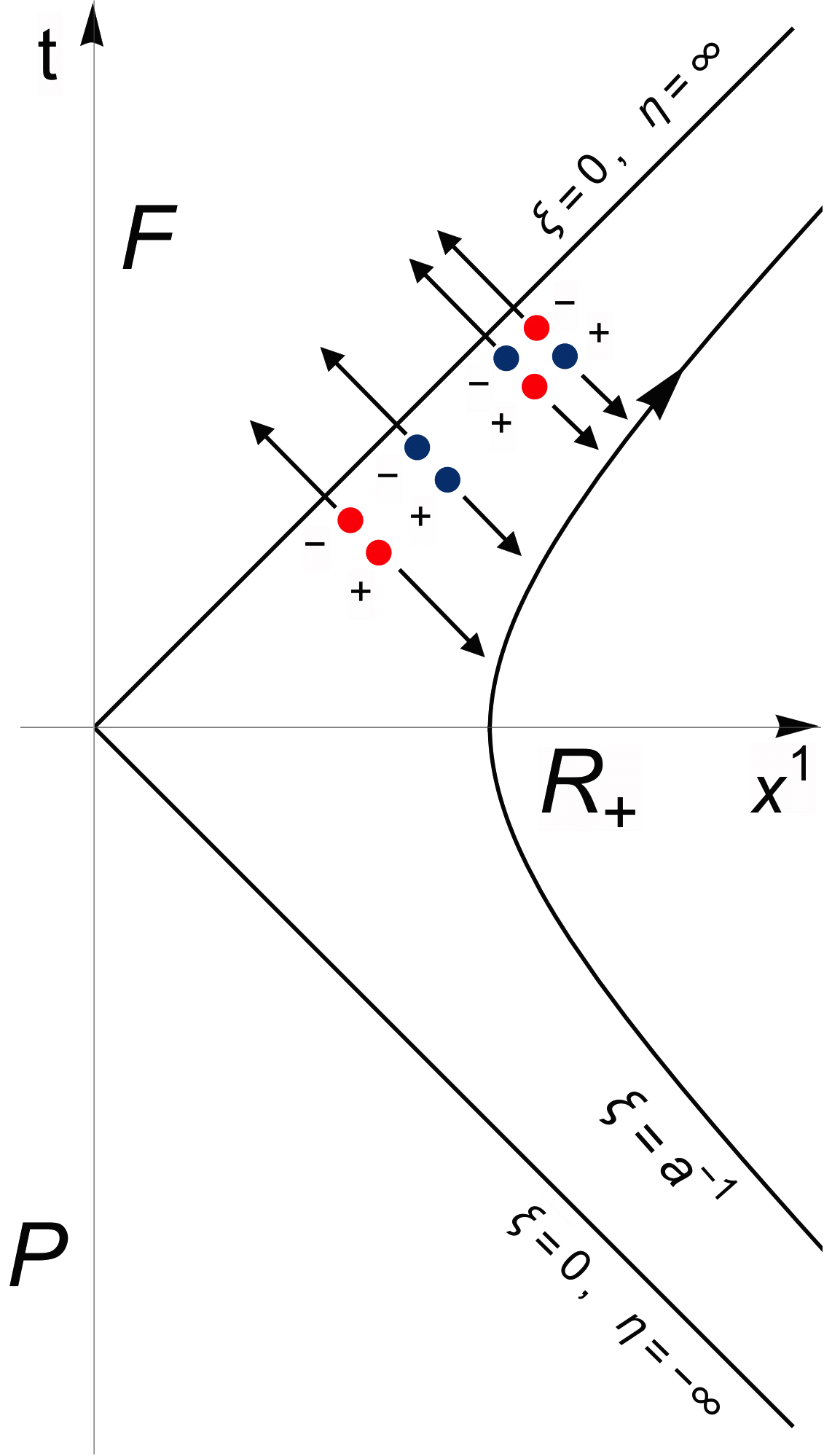
Figure 2: Pictorial interpretation of Unruh spectrum for mixed fields. Different (online) dot colors correspond to different particle-antiparticle flavors. Unruh effect originates from quantum vacuum fluctuations close to Rindler horizon. In the absence of mixing, vacuum contains a single type of particle-antiparticle pairs (either blue-blue or red-red). Conversely, for mixed fields hybrid types of pairs (red-blue and blue-red) do appear as well. This spoils the characteristic particle spectrum, which can be approximately identified with the $q$-generalized Bose-Einstein condensate based on Tsallis entropy.

From the above considerations, we infer that the correlations induced by mixing do spoil the macroscopic properties of Unruh thermal condensate by affecting the statistical behavior of its microscopic configurations. This gives rise to an entangled condensate structure of both equal and hybrid particle-antiparticle pairs that obey the nonadditive Tsallis entropy law in a suitable limit. Remarkably, we notice that nonextensive statistics based on Tsallis entropies have been largely used in the study of entanglement TSENT , such as the relative entropy and the Peres criterion.

The above result is quite general, since it is not confined to bosons solely. In NonTN the Unruh effect has been investigated in the case of mixing of (Dirac) fermions, and in particular of neutrinos, showing that the vacuum condensate of Rindler particles should be modified as (see Eq. (23) of NonTN )

$$\mathcal{N}_{\theta,\Delta m}(\Omega_{n})\,=\,N_{\mathrm{FD}}(\Omega_{n})\,+\,\sin^{2}\theta\,\,\mathcal{O}\left(\frac{|\Delta m^{2}|}{\mu^{2}_{k,1}}\right)\,=\,\frac{1}{e^{2\pi\Omega_{n}}+1}\,+\,\sin^{2}\theta\,\,\mathcal{O}\left(\frac{|\Delta m^{2}|}{\mu^{2}_{k,1}}\right),$$ (42)

where the zeroth-order term is now given by the Fermi-Dirac distribution function, while the higher-order corrections $\mathcal{O}\left({|\Delta m^{2}|}/{\mu^{2}_{k,1}}\right)$ depend on the convolution integral of the condensation density of mass vacuum in such a way that the Pauli principle is still satisfied. In particular, we have NonTN

$$\hskip 75.39963pt\mathcal{O}\left(\frac{|\Delta m^{2}|}{\mu^{2}_{k,1}}\right)\,=\,\frac{e^{\pi\Omega_{n}}}{2\hskip 0.28453pt\cosh\left(\pi\Omega_{n}\right)}\hskip 2.56073ptN_{F,F}(\Omega_{n})\,-\,\frac{e^{-\pi\Omega_{n}}}{2\hskip 0.28453pt\cosh\left(\pi\Omega_{n}\right)}\hskip 2.56073ptN_{G,G}(\Omega_{n})\,,$$ (43)

$$N_{F,F}(\Omega_{n})=\sum_{r=1,2}\int\,F^{\hskip 0.56905pt*}_{r}(k_{1},\Omega_{n})\,F_{r}(k_{1},\Omega_{n})\,{|V_{\bf{k}}|}^{2},\quad\,\,N_{G,G}(\Omega_{n})=\sum_{r=1,2}\int\,G^{\hskip 0.56905pt*}_{r}(k_{1},\Omega_{n})\,G_{r}(k_{1},\Omega_{n})\,{|V_{\bf{k}}|}^{2}.$$ (44)

Here $F_{r}$ and $G_{r}$ are proper combinations of Dirac modes of spin $r$ in Minkowski and Rindler quantizations NonTN and

$$V_{\bf{k}}(t)=\left(\frac{\omega_{{\bf k},1}+m_{1}}{2\omega_{{\bf k},1}}\right)^{\frac{1}{2}}\left(\frac{\omega_{{\bf k},2}+m_{2}}{2\omega_{{\bf k},2}}\right)^{\frac{1}{2}}\left(\frac{|{\bf k}|}{\omega_{{\bf k},2}+m_{2}}-\frac{|{\bf k}|}{\omega_{{\bf k},1}+m_{1}}\right)\,e^{i(\omega_{{\bf k},2}+\omega_{{\bf k},1})\,t},$$ (45)

is the analogue of the Bogoliubov coefficient ${\lambda}^{\bf{k}}_{12}(t)$ in Eq. (57) for fermion mixing BV95 (we have assumed for simplicity $\textbf{k}=(k_{1},0,0))$. Once more, it is easy to check that Eq. (46) reproduces the standard result for $\theta\rightarrow 0$ and/or $m_{1}\rightarrow m_{2}$, consistently with the absence of mixing in both cases. The same holds in the quantum mechanical limit of large momenta with respect to the mass difference, since the condensation density $|V_{\bf{k}}|^{2}\rightarrow 0$.

At the same time, the $q$-modified Fermi-Dirac distribution in Tsallis thermostatistics can be approximately written as Buyu3

$$N_{q}(\epsilon_{n})=\frac{1}{\left[1+(q-1)\beta\epsilon_{n}\right]^{1/(q-1)}+1}\,.$$ (46)

Therefore, by expanding for small deviations of $q$ from unity and following the same reasoning as earlier, we arrive at a relation akin to Eq. (40) for fermions. Clearly, such an extension deserves careful attention, since neutrinos are the most abundant and emblematic example of mixed particles.

V Conclusions and Outlook

The Unruh effect predicts that a uniformly accelerated observer measures a Planck emission distribution in Minkowski vacuum. However, for quantum fields exhibiting entanglement correlations induced by mixing, this result turns out to be nontrivially spoilt Luciano ; NonTN . Here we have discussed this phenomenon from a statistical point of view. Working in the approximation of small mass difference between the mixed fields, we have shown that the modified vacuum distribution can be modeled by the $q$-generalized Bose-Einstein distribution based on the nonadditive Tsallis entropy. In this effective description, the deviation from Planckianity is found to be quantified by the mixing angle $\theta$ and the mass difference $\Delta m$. Furthermore, the $q$-entropic index exhibits a running behavior, which is reasonably expected for QFT systems as discussed in App13 . The outcome that $q<1$ indicates that we are in the superadditive regime of Tsallis statistics, consistently with the appearance of both equal and hybrid particle-antiparticle pairs in the vacuum.

Apart from more formal aspects, we remark that the above picture allows us to extend the peculiar thermal features of Unruh effect to mixed fields. Indeed, in Luciano ; NonTN flavor mixing was seen as responsible for the emergence of nonthermal contributions in the Unruh spectrum. Here we have proved that the origin of these extra terms can be explained in terms of a departure of the vacuum distribution from Boltzmann-Gibbs statistics. In turn, this phenomenon is attributable to the complex structure acquired by the vacuum state for mixed fields, which becomes a condensate of entangled particle-antiparticle pairs of different species. In other words, we can still identify a temperature for the vacuum distribution, provided that we work in the framework of Tsallis’s thermostatistics. Nevertheless, following AbePla we point out that the new physical temperature would be different from Unruh temperature by a factor depending on the nonextensivity $q$-parameter and the modified entropy $S_{q}$, in such a way that the usual result is still recovered for $q\rightarrow 1$. In this regard, we mention that a similar $q$-dependent expression for Unruh temperature in Tsallis’s theory has been obtained in Shababi in the context of the Generalized Uncertainty Principle. Possible connections between the two results need further consideration and will be addressed elsewhere.

In passing, we highlight that a nonthermal behavior of Unruh effect has been recently exhibited in Dop even for the case of a single (i.e. unmixed) massive field. In that case, it has been found that, contrary to what happens with a linear dispersion relation characteristic of massless fields, the thermality of Unruh condensate would be lost for more general dispersion relations including a mass term, unless one defines a varying apparent Unruh temperature depending on both the acceleration and the degree of departure from linearity. Therefore, it would be interesting to investigate whether such a result interfaces with our reformulation of Unruh effect in Tsallis’s language. For this purpose, however, a formalism based on the relativistic Doppler shift method is required Dop , since the Bogoliubov transformation approach is insensitive to the mass of the field when computing Unruh vacuum distribution Takagi .

Beyond the above issues, several other aspects remain to be analyzed. To avoid unnecessary technicalities, we have focused on a simplified model involving only two scalar fields, noticing that similar considerations can be extended to fermions quite straightforwardly. Furthermore, our perturbative analysis relies on the leading-order approximation of small difference between the masses of mixed fields. The question thus arises as to how the connection (40) between the nonextensive $q$-index and the mixing parameters would appear for arbitrary mass differences, as well as in the case of three flavor generations. Another extension is to apply the above formalism to the best-known Hawking radiation, which has been largely studied within the framework of nonextensive corrected-entropies in recent years Barrow .

From a more phenomenological perspective, it would be challenging to test possible experimental implications of our result. As well known, direct evidences of Unruh effect have not yet been obtained, the obvious reason being the fact that the Unruh temperature is extremely small even for huge accelerations. However, there have been many proposals in the literature to bypass hindrances arising from technical limitations by focusing on analogues of Unruh effect, even at the classical level. For instance, feasible tests are being analyzed by simulating vacuum fluctuations of Minkowski spacetime through gravity waves on the surface of water subject to white noise Leona . Attempts to detect indirect traces of Unruh radiation have also been carried out in graphene graphene and metamaterials Smoly , where the effects of Rindler-like horizons are mimicked by means of photons waveguides. Thus, such analog models provide the only test bench for probing the Unruh effect and any possible deviation from the standard behavior to date.

Finally, one more direction to explore is whether Tsallis statistics and mixed particles are intertwined on a more fundamental level that goes beyond the specific framework of Unruh effect. In this vein, we emphasize the recent proposal to solve the long-standing problem of abundance of primordial ${}^{7}\mathrm{Li}$, which is affected by the neutrino interactions and primordial magnetic field, by investigating the impact of Big Bang nucleosynthesis predictions of adopting a Tsallis distribution for the nucleon energies Litium . Work along the above research lines is presently under active consideration.

Appendix A QFT of flavor mixing in Minkowski spacetime

We review the QFT formalism of flavor mixing for the simplest case of two scalar fields in Minkowski background BlasCap . Toward this end, we introduce the algebraic generator of mixing

$$G_{\theta}(t)=\exp\left[-i\theta\int d^{3}x\hskip 0.56905pt\Big{(}\pi_{1}(x)\phi_{2}(x)\,-\,\pi_{2}(x)\phi_{1}(x)\Big{)}\right],$$ (47)

where the notation has already been set up in Sec. III. In terms of this operator, the mixing transformations in Eqs. (21) and (22) can be cast as

$$\phi_{\ell}(x)=G_{\theta}^{-1}(t)\phi_{j}(x)G_{\theta}(t)\,,$$ (48)

where $(\ell,j)=\left\{(A,1),(B,2)\right\}$. One can prove that $G_{\theta}(t)$ belongs to $SU(2)$ group, the algebra of which is closed by the operators BlasCap

$$S_{+}(t)=-i\int d^{3}x\hskip 1.99168pt\pi_{1}(x)\phi_{2}(x)\,,\quad S_{-}(t)=-i\int d^{3}x\hskip 1.99168pt\pi_{2}(x)\phi_{1}(x)\,,$$ (49)

$$S_{3}=-\frac{i}{2}\int d^{3}x\hskip 1.99168pt\Big{(}\pi_{1}(x)\phi_{1}(x)-\pi_{2}(x)\phi_{2}(x)\Big{)}\,,\quad S_{0}=-\frac{i}{2}\int d^{3}x\hskip 1.99168pt\Big{(}\pi_{1}(x)\phi_{1}(x)+\pi_{2}(x)\phi_{2}(x)\Big{)}\,.$$ (50)

Within the framework of QFT mixing, the generator (47) plays a pivotal rôle, as it provides the dynamical map between the Fock space $\mathcal{H}_{A,B}$ for the fields with definite flavor and the Fock space $\mathcal{H}_{1,2}$ for the fields with definite mass. Indeed, let us consider the generic matrix element of $\mathcal{H}_{1,2}\,=\mathcal{H}_{1}\otimes\mathcal{H}_{2}$, i.e. ${}_{1,2}\langle a|\phi_{i}(x)|b\rangle_{1,2}$ ($i=1,2$), where $|a\rangle_{1,2}$ and $|b\rangle_{1,2}$ are arbitrary states in ${\mathcal{H}}_{1,2}$. By inverting Eq. (48) with respect to $\phi_{j}$, we get

$${}_{1,2}\langle a|G_{\theta}(t)\hskip 0.56905pt\phi_{\ell}(x)\hskip 0.56905ptG^{-1}_{\theta}(t)|b\rangle_{1,2}=\hskip 0.28453pt_{1,2}\langle a|\phi_{j}(x)|b\rangle_{1,2}\,,$$ (51)

which in fact shows that $G_{\theta}^{-1}(t)|b\rangle_{1,2}$ is a vector in $\mathcal{H}_{A,B}$. Therefore, we can write

$$G^{-1}_{\theta}(t):{\mathcal{H}}_{1,2}\mapsto{\mathcal{H}}_{A,B}\,.$$ (52)

In particular, for the vacuum state $|0_{\mathrm{M}}\rangle_{1,2}\equiv|0\rangle_{1,2}=|0\rangle_{1}\otimes|0\rangle_{2}$, this gives

$$|0(\theta,t)\rangle_{A,B}=G^{-1}_{\theta}(t)|0\rangle_{1,2}\,.$$ (53)

The above relation allows us to define the time-dependent flavor vacuum $|0(\theta,t)\rangle_{A,B}$ in terms of the corresponding mass vacuum $|0\rangle_{1,2}$.

A comment is in order here. For quantum mechanical systems (i.e. systems with finite number of degrees of freedom), $G_{\theta}(t)$ is a unitary operator that preserves the canonical commutation relations. This is ensured by Stone-von Neuman theorem SvN ; Stone , which states that any two irreducible representations of the canonical commutators are unitarily equivalent in Quantum Mechanics. Accordingly, mass and flavor representations give rise to physically equivalent descriptions of mixing. On the other hand, in QFT the transformation (47) is found to be nonunitary in the infinite volume limit, which means that the vacua $|0\rangle_{1,2}$ and $|0(t)\rangle_{A,B}$ become mutually orthogonal and the related Fock spaces unitarily inequivalent. This is quite different from the conventional perturbation theory, where the vacuum of the interacting theory is expected to be essentially the same as that of the free theory (up to a phase factor) BogoCit . Clearly, such an inequivalence and its implications disappear for $\theta=0$ and/or $m_{2}=m_{1}$, consistently with the fact that there is no mixing in both cases.

To find out how the mapping (53) affects the structure of the flavor vacuum, we now focus on the derivation of ladder operators in the flavor basis. By using the standard plane-wave quantization (7) for both $\phi_{1}$ and $\phi_{2}$, Eq. (48) leads to the following expansions for the flavor fields

$$\phi_{\ell}(x)=\int d^{3}{k}\hskip 0.56905pt\Big{\{}a_{\textbf{k},\ell}(\theta,t)\,U_{\textbf{k},j}(x)+\bar{a}_{\textbf{k},\ell}^{\dagger}(\theta,t)\,U_{\textbf{k},j}^{\hskip 0.28453pt*}(x)\Big{\}},\,\,\quad(\ell,j)=\left\{(A,1),(B,2)\right\},$$ (54)

where

$$a_{\textbf{k},\ell}(\theta,t)\,\equiv\,G^{-1}_{\theta}(t)\hskip 0.56905pta_{\textbf{k},j}\hskip 0.56905ptG_{\theta}(t)\,,$$ (55)

is the annihilator of a quantum with definite flavor $\ell$ (for simplicity, we refer to this operator as flavor annihilator and use the handier notation $a_{\textbf{k},\ell}(\theta,t)\equiv a_{\textbf{k},\ell}(t)$). From the above relation, we obtain

$$a_{{{\bf{k}}},A}(t)=\cos\theta\,a_{{{\bf{k}}},1}\,+\,\sin\theta\,\left({\rho}^{\bf{k}\,*}_{12}(t)\,a_{{{\bf{k}}},2}\,+\,{\lambda}^{\bf{k}}_{12}(t)\,\bar{a}^{\dagger}_{-{{\bf{k}}},2}\right),$$ (56)

(similarly for $a_{\textbf{k},B}(\theta,t))$. Therefore, the flavor annihilator is related to the corresponding ladder operators in the mass basis via of a Bogoliubov transformation (the terms in the brackets) nested into a rotation. The Bogoliubov coefficients are defined as

$${\rho}^{\bf{k}}_{12}(t)=|{\rho}^{\bf{k}}_{12}|\,e^{i\left(\omega_{{\bf{k}},2}-\omega_{{\bf{k}},1}\right)t}\,,\quad{\lambda}^{\bf{k}}_{12}(t)=|{\lambda}^{\bf{k}}_{12}|\,e^{i\left(\omega_{k,1}+\omega_{k,2}\right)t}\,,$$ (57)

where

$$|{\rho}^{\bf{k}}_{12}|\equiv\frac{1}{2}\left(\sqrt{\frac{\omega_{{\bf{k}},1}}{\omega_{{\bf{k}},2}}}\,+\,\sqrt{\frac{\omega_{{\bf{k}},2}}{\omega_{{\bf{k}},1}}}\right),\qquad|{\lambda}^{\bf{k}}_{12}|\equiv\frac{1}{2}\left(\sqrt{\frac{\omega_{{\bf{k}},1}}{\omega_{{\bf{k}},2}}}\,-\,\sqrt{\frac{\omega_{{\bf{k}},2}}{\omega_{{\bf{k}},1}}}\right).$$ (58)

It is easy to verify that

$${|{\rho}^{\bf{k}}_{12}|}^{2}\,-\,{|{\lambda}^{\bf{k}}_{12}|}^{2}=1\,,$$ (59)

which ensures that the flavor operator (55) and its conjugate are still canonical (at equal times).

The mapping (53) induces a physically nontrivial structure in the flavor vacuum, which becomes an entangled $SU(2)$ coherent state made up by particle-antiparticle pairs both of the same and different masses BV95 . In turn, this inequivalence affects the well-known oscillation formula to include the antiparticle degrees of freedom BlasPlb . The condensation density of flavor vacuum is given by

$${}_{A,B}\langle 0(t)|a_{{{\bf{k}}^{\prime}},i}^{\dagger}\,a_{{\bf k},j}|0(t)\rangle_{A,B}=\sin^{2}\theta\;{|{\lambda}^{\bf{k}}_{12}|}^{2}\delta_{ij}\delta^{3}({\textbf{k}-\textbf{k}^{\prime}})\,.$$ (60)

Clearly, by exploiting the symmetric structure of Eq. (55), one can reverse the above reasoning and analyze the properties of mass vacuum, which appears as a condensate of particle-antiparticle pairs having both equal and different flavors. In line with our previous considerations on the disappearance of the inequivalence for vanishing mixing, the condensation density (60) goes to zero for $\theta=0$ (since $a_{{\bf{k}},A}\rightarrow a_{{\bf{k}},1}$ and $a_{{\bf{k}},B}\rightarrow a_{{\bf{k}},2}$) and/or $m_{2}=m_{1}$ (since the Bogoliubov coefficients reduce to ${\rho}^{\bf{k}}_{12}(t)=1$ and ${\lambda}^{\bf{k}}_{12}(t)=0$, which in turn implies that $a_{{\bf{k}},A}$ and $a_{{\bf{k}},B}$ are simple superpositions of $a_{{\bf{k}},1}$ and $a_{{\bf{k}},2}$). Notice that the same behavior occurs for ${|{\bf{k}}|}^{2}\gg\frac{{m_{1}}^{2}+{m_{2}}^{2}}{2}$, thus allowing to recover the standard quantum mechanical description of mixing in the relativistic approximation.

The complex structure of the flavor vacuum $|0(t)\rangle_{A,B}$ has been recently studied in Cabo , where it has been established that the Fock space for flavor fields cannot be obtained by the direct product of the spaces for massive fields. This strengthen the result that entanglement properties for mixed fields already emerge at the level of vacuum state. As a remark, the observation that flavor mixing can be associated with (single-particle) entanglement traces back to Dimauro and has inspired a series of studies on violations of Bell, Leggett-Garg and Mermin-Svetchlichny inequalities, nonlocality, gravity-acceleration degradation effects and other similar phenomena SimPhe1 ; SimPhe2 ; SimPhe3 ; SimPhe4 ; SimPhe5 . The entanglement content of the flavor vacuum has been explicitly quantified in Vacent in the limit of small mass difference and/or mixing angle.

References

M. Kobayashi and T. Maskawa, Prog. Theor. Phys. 49, 652 (1973).

N. Cabibbo, Phys. Rev. Lett. 10, 531 (1963).

Y. Fukuda et al. [Super-Kamiokande], Phys. Rev. Lett. 81, 1562 (1998); K. Abe et al. [Super-Kamiokande], Phys. Rev. Lett. 110, 181802 (2013).

Q. R. Ahmad et al. [SNO], Phys. Rev. Lett. 87, 071301 (2001); Q. R. Ahmad et al. [SNO], Phys. Rev. Lett. 89, 011301 (2002).

S. M. Bilenky and B. Pontecorvo, Phys. Rept.  41, 225 (1978).

M. Blasone and G. Vitiello, Annals Phys.  244, 283 (1995).

M. Blasone, A. Capolupo, O. Romei and G. Vitiello, Phys. Rev. D 63, 125015 (2001).

A. Cabo Montes de Oca and N. G. Cabo Bizet, [arXiv:2005.07758 [hep-ph]].

M. Blasone, G. Lambiase and G. G. Luciano, Phys. Rev. D 96, 025023 (2017).

M. Blasone, G. Lambiase and G. G. Luciano, J. Phys. Conf. Ser. 956, 012021 (2018).

A. Capolupo, G. Lambiase and A. Quaranta, Phys. Rev. D 101, 095022 (2020).

W. G. Unruh, Phys. Rev. D 14, 870 (1976).

J. Marino, A. Noto and R. Passante, Phys. Rev. Lett. 113, 020403 (2014).

F. Hammad, A. Landry and D. Dijamco, Accepted for publication in Physical Review D [arXiv:2102.08944 [gr-qc]].

F. Scardigli, M. Blasone, G. Luciano and R. Casadio, Eur. Phys. J. C 78, 728 (2018).

G. G. Luciano and L. Petruzziello, Eur. Phys. J. C 79, 283 (2019).

M. Blasone, G. Lambiase, G. G. Luciano and L. Petruzziello, Phys. Rev. D 97, 105008 (2018).

M. Blasone, G. Lambiase, G. G. Luciano and L. Petruzziello, Phys. Lett. B 800, 135083 (2020).

M. Blasone, G. Lambiase, G. G. Luciano and L. Petruzziello, Eur. Phys. J. C 80, 130 (2020).

C. Tsallis, J. Stat. Phys. 52, 479 (1988).

C. Tsallis, Introduction to Non-Extensive Statistical Mechanics: Approaching a Complex World, Springer, Berlin, 2009.

C. Tsallis and L. J. L. Cirto, Eur. Phys. J. C 73, 2487 (2013).

M. L. Lyra and C. Tsallis, Phys. Rev. Lett. 80, 53 (1998).

A. R. Plastino and A. Plastino, Phys. Lett. A 174, 384 (1993).

V. H. Hamity and D. E. Barraco, Phys. Rev. Lett. 76, 4664 (1996).

C. Tsallis, F. C. Sa Barreto and E. D. Loh, Phys. Rev. E 52, 1447 (1995).

A. R. Plastino, A. Plastino and H. Vucetich, Phys. Lett. A 207, 42 (1995).

G. Kaniadakis, A. Lavagno and P. Quarati, Phys. Lett. B 369, 308 (1996).

P. Jizba, J. Korbel and V. Zatloukal, Phys. Rev. E 95, 022103 (2017).

S. Nojiri, S. D. Odintsov and E. N. Saridakis, Eur. Phys. J. C 79, 242 (2019).

E. M. Barboza, Jr., R. d. Nunes, E. M. C. Abreu and J. Ananias Neto, Physica A 436, 301 (2015).

A. Rényi, Proceedings of the fourth Berkeley Symposium on Mathematics, Statistics and Probability 1960, 547 (1961); G. Kaniadakis, Phys. Rev. E 66, 056125 (2002).

V. F. Mukhanov and S. Winitzki, Introduction to Quantum Effects in Gravity, Cambridge University Press, Cambridge, 2007.

S. Takagi, Prog. Theor. Phys. Suppl. 88, 1 (1986).

S. Hawking, Commun. Math. Phys. 43, 199 (1975).

C. R. Ji and Y. Mishchenko, Phys. Rev. D 64, 076004 (2001).

F. Büyükkiliç and D. Demirhan, Phys. Lett. A 181, 24 (1993).

F. Büyükkiliç, D. Demirhan and A. Güleç, Phys. Lett. A 197, 209 (1995).

U. Timakli, F. Büyükkiliç and D. Demirhan, Physica A 240, 657 (1997).

Q.A. Wang, M. Pezeril, A. Le Mèhautè, Physica A 278, 337 (2000).

J. Chen, Z. Zhang, G. Su, L. Chen and Y. Shu, Phys. Lett. A 300, 65 (2002).

Q.A. Wang and Le Mèhautè, Phys. Lett. A 235, 222 (1997).

H. Shababi and K. Ourabah, Eur. Phys. J. Plus 135, 697 (2020).

H. Moradpour, C. Corda and A. H. Ziaie, [arXiv:2012.08316 [gr-qc]].

P. A. Zyla et al. [Particle Data Group], PTEP 2020, 083C01 (2020).

S. Abe and A. K. Rajagopal, Phys. Rev. A 60, 3461 (1999); C. Tsallis, S. Lioyd, and M. Baranger, Phys. Rev. A63, 042104 (2001); N. Canosa and R. Rossignoli, Phys. Rev. Lett. 88, 170401 (2002).

S. Abe, S. Martínez, F. Pennini and A. Plastino, Phys. Lett. A 281, 126 (2001).

T. S. Biró and V. G. Czinner, Phys. Lett. B 726, 861-865 (2013); E. M. C. Abreu and J. A. Neto, Phys. Lett. B 810, 135805 (2020); A. Alonso-Serrano, M. P. Dabrowski and H. Gohar, Phys. Rev. D 103, 026021 (2021).

U. Leonhardt, I. Griniasty, S. Wildeman, E. Fort and M. Fink, Phys. Rev. A 98, 022118 (2018).

A. Iorio and G. Lambiase, Phys. Lett. B 716, 334 (2012).

I. I. Smolyaninov, Opt. Lett. 44, 2224 (2019).

S. Q. Hou, J. J. He, A. Parikh, D. Kahl, C. A. Bertulani, T. Kajino, G. J. Mathews and G. Zhao, Astrophys. J. 834, 165 (2017).

J. von Neumann, Mat. Ann. 104, 570 (1931).

M. H. Stone, Ann. Math. 33, 643 (1932).

N. Bogoliubov and D. Shirkov Introduction to the theory of quantized fields, New York: John Wiley, 1980.

M. Blasone, P. A. Henning and G. Vitiello, Phys. Lett. B 451, 140 (1999).

M. Blasone, F. Dell’Anno, S. De Siena, M. Di Mauro and F. Illuminati, Phys. Rev. D 77, 096002 (2008); M. Blasone, F. Dell’Anno, S. De Siena and F. Illuminati, EPL 106, 30002 (2014).

S. Banerjee, A. K. Alok, and R. MacKenzie, Eur. Phys. J. Plus 131, 129 (2016).

V. A. S. V. Bittencourt, C. J. Villas Boas, and A. E. Bernardini, Europhys. Lett. 108, 50005 (2014).

X. K. Song, Y. Huang, J. Ling, and M. H. Yung, Phys. Rev. A 98, 050302(R) (2018).

J. Naikoo, A. K. Alok, S. Banerjee, and S. U. Sankar, Phys. Rev. D 99, 095001 (2019).

K. Dixit, J. Naikoo, B. Mukhopadhyay, and S. Banerjee, Phys. Rev. D 100, 055021 (2019).

M. Blasone, F. Illuminati, G. G. Luciano and L. Petruzziello, Phys. Rev. A 103, 032434 (2021).