A Hamiltonian Mechanics Framework for Charge Particle Optics in Straight and Curved Systems

Abstract

Charged particle optics, the description of particle trajectories in the vicinity of some optical axis, describe the imaging properties of particle optics devices. Here, we present a complete and compact description of charged particle optics employing perturbative expansion of Hamiltonian mechanics. The derived framework allows the straightforward computation of transversal and longitudinal (chromatic) properties of static and dynamic optical devices with straight and curved optical axes. It furthermore gives rise to geometric integration schemes preserving the symplectic phase space structure and pertaining Lagrange invariants, which may be employed to derive analytic approximations of aberration coefficients and efficient numerical trajectory solvers.

I Introduction

Charged particle optical (CPO) systems such as particle accelerators, electron or ion microscopes, focussed ion beam instruments, or lithography machines rely on tailored electromagnetic field configurations to realize optical imaging with charged particles. The goal is to create a controllable and well-defined mapping between entrance and exit plane of the device. This can be typically described well within the framework of (relativistic) classical mechanics as quantum effects (e.g., spin-orbit coupling) are generally small. Moreover, one does not need the general description of all possible particle trajectories in a given field configuration; those close to the optical axis are generally sufficient. For instance, the paraxial approximation, which describes first order deviations of trajectories with respect to the optical axis already entails the principal properties of the optical system. Unfortunately, the large numerical apertures and beam diameters used in modern CPO devices typically requires consideration of trajectories beyond the paraxial, i.e., linear, limit. These trajectories determine the aberrations limiting the optical performance of the device (e.g., spatial resolution, beam collimation or energy filter transparency). Although modern computational methods allow numerical evaluation of arbitrary trajectories at high speed and accuracy, perturbation methods computing path deviations in a semianalytical way are indispensible tools as they provide categorical properties, e.g., symmetries canceling out certain aberrations, and parametric models, e.g., for refining field configurations. The most common analytical perturbation methods are the trajectory method, the eikonal method and the Lie algebra method. The trajectory method iteratively solves Newton’s equations of motion [1], the eikonal method [2, 3, 4, 5] iterates Hamiltonian characteristic functions (here called the eikonal) with respect to trajectory deviations, and the Lie algebra method [6, 7, 8] is based on the canonical perturbation method in phase space [9, 10]. A comprehensive comparison of these methods in electron optics has been carried out by T. Radlicka [11].

In spite of the longstanding and successful use of the above approaches, they also have some shortcomings, which, e.g., prevent a compact description and complicate the treatment of curvilinear systems. Indeed, chromatic aberrations are frequently derived by a separate variation of the trajectories with respect to the particles energy and in devices with with a curved optical axis curved coordinate systems (e.g., defined by moving Frenet trihedrals) are employed (e.g., [12]). Both approaches (although perfectly viable from a theoretical point of view) come as auxiliary modifications, frequently leading to significant mathematical and computational complexity. We therefore provide for yet another perturbation approach in the following, which leads to very compact and straightforward expressions irrespective of the particular shape of the CPO system, the fields, considered deviation parameters or the chosen coordinate system.

Our approach is rooted in Hamiltonian mechanics exploiting the perturbation framework leading to the so-called Jacobi variational equation (JVE) in the first order [13]. The approach naturally makes use of the symplectic structure of classical mechanics (i.e., conservation of phase space), allowing, for example, the use of efficient geometrical integration schemes in the calculation of optical properties from given field configurations. In that, the approach shares a number of similarities with the Lie algebraic methods [14, 6], indeed it may be regarded as a compactified version thereof.

In the following, we will shortly recapitulate the basics of Hamiltonian mechanics for charged particles including perturbation series expansion of the Hamiltonian equations of motion. We then explicitly carry out the linear perturbation for electric and magnetic fields in both the non-relativistic and relativistic regime and discuss the structure and general properties of the ensuing paraxial equations. In the subsequent section higher-order expansions are demonstrated. In the Appendix we discuss some of the most important CPO elements, namely magnetic quadrupole, round magnetic lens, Wien filter and sector magnet, to illustrate the developed formalism.

II Fundamentals of Hamiltonian Mechanics

To describe the motion of a charged particle in an electromagnetic field we employ Hamiltonian mechanics, which operates in phase space endowed with phase space coordinates for position $\boldsymbol{r}$ and canonical momentum $\boldsymbol{p}$. The non-relativistic Hamiltonian, corresponding to the total energy of the system, reads

$$\mathcal{H}\left(\boldsymbol{r},\boldsymbol{p},t\right)=\frac{\left(\boldsymbol{p}-q\boldsymbol{A}\left(\boldsymbol{r},t\right)\right)^{2}}{2m}+q\Phi\left(\boldsymbol{r},t\right)$$ (1)

Here, $m$, $q$, $\boldsymbol{A}$, and $\Phi$ denote the particle’s mass, charge, as well as the magnetic vector potential and electric potential, respectively. As charged particle optics frequently deals with relativistic particles we also note the relativistic Hamiltonian

$${\displaystyle\mathcal{H}} =\sqrt{m^{2}c^{4}+\left(\mathbf{p}-q\mathbf{A}\right)^{2}c^{2}}+q\Phi$$ (2)

$$=\gamma mc^{2}+q\Phi\,,$$

where we omitted the coordinate arguments to shorten notation. In the following derivation, however, we resort to the non-relativistic expressions for simplicity. Relevant relativistic expressions will be given at the end of the next section. Hamilton’s equations of motion read

$$\frac{d\boldsymbol{x}}{dt}=\begin{pmatrix}\frac{d\boldsymbol{r}}{dt}\\ \frac{d\boldsymbol{p}}{dt}\end{pmatrix}=\left\{\boldsymbol{x},\mathcal{H}\right\}=\begin{pmatrix}\frac{\partial\mathcal{H}}{\partial\boldsymbol{p}}\\ -\frac{\partial\mathcal{H}}{\partial\boldsymbol{r}}\end{pmatrix}=\boldsymbol{X}_{\boldsymbol{x}\left(t\right)}\,,$$ (3)

where we introduced typically 6-dimensional phase space coordinates $\boldsymbol{x}\coloneqq\left(\boldsymbol{r},\boldsymbol{p}\right)^{T}$, the Poisson bracket $\left\{\cdot,\cdot\right\}$, and the Hamiltonian vector field

$$\boldsymbol{X}_{\boldsymbol{x}\left(t\right)}\coloneqq\begin{pmatrix}\frac{\boldsymbol{p}-q\boldsymbol{A}}{m}\\ \frac{q}{m}\frac{\partial A_{i}}{\partial\boldsymbol{r}}\left(p_{i}-qA_{i}\right)-q\frac{\partial\Phi}{\partial\boldsymbol{r}}\end{pmatrix}\,.$$ (4)

Here and henceforth, Einstein summation convention is employed.

In CPO we describe the motion of a charged particle in the vicinity of some given optical axis (also referred to as the design trajectory), which is an exact solution to the full equations of motion. That can be a straight optical axis as, e.g., the symmetry axis of a round magnetic lens, or a curved axis as, e.g., a circular reference trajectory in a sector magnet. The Lie algebraic methods use the second equality in (3) as starting point for an iterative solution facilitated by a Taylor expansion of the Hamiltonian around the the optical axis. This formalism involves the use of some operator algebra and canonical transformations to the design trajectory. In the following we essentially present a shortcut yielding the same results based on directly considering the variation of particle trajectory $\delta\boldsymbol{x}$ around the optical axis trajectory $\boldsymbol{x}\left(t\right)$ in phase space

$$\boldsymbol{y}\left(t\right)=\boldsymbol{x}\left(t\right)+\delta\boldsymbol{x}\left(t\right)\,.$$ (5)

Hamilton’s equations of motion for such trajectories read

$$\frac{d\left(\boldsymbol{x}+\delta\boldsymbol{x}\right)}{dt}=\boldsymbol{X}_{\boldsymbol{x}+\delta\boldsymbol{x}}$$ (6)

yielding the following difference to the optical axis trajectory

$$\frac{d\left(\boldsymbol{x}+\delta\boldsymbol{x}\right)}{dt}-\frac{d\boldsymbol{x}}{dt} =\frac{d\left(\delta\boldsymbol{x}\right)}{dt}$$ (7)

$$=\boldsymbol{X}_{\boldsymbol{x}+\delta\boldsymbol{x}}-\boldsymbol{X}_{\boldsymbol{x}}$$

We now expand the deviation into a perturbation series, $\delta\boldsymbol{x}=\sum_{n}\varepsilon^{n}\delta\boldsymbol{x}^{\left(n\right)}$, with an artificial smallness parameter $\varepsilon=1$, indicating the smallness of the deviation vector $\delta\boldsymbol{x}^{\left(n\right)}$ and develop the right hand side of (7) into a multidimensional Taylor series

$$\frac{d\left(\sum_{n}\varepsilon^{n}\delta x_{i}^{(n)}\right)}{dt} =\left(\frac{\partial X_{i}}{\partial x_{j}}\right)_{\boldsymbol{x}\left(t\right)}\sum_{n}\varepsilon^{n}\delta x_{j}^{\left(n\right)}$$ (8)

$$+\frac{1}{2}\left(\frac{\partial^{2}X_{i}}{\partial x_{j_{1}}\partial x_{j_{2}}}\right)_{\boldsymbol{x}\left(t\right)}\sum_{n_{1}}\varepsilon^{n_{1}}\delta x_{j_{1}}^{\left(n_{1}\right)}\sum_{n_{2}}\varepsilon^{n_{2}}\delta x_{j_{2}}^{\left(n_{2}\right)}$$

$$+\ldots$$

$$=\sum_{n=1}^{\infty}\frac{1}{n!}\sum_{\left|j\right|=n}\begin{pmatrix}n\\ j\end{pmatrix}\left(D^{j}X_{i}\right)_{\boldsymbol{x}\left(t\right)}\left(\sum_{m}\varepsilon^{m}\delta x^{\left(m\right)}\right)^{j}\,.$$

In the last line we employed multiindex notation $j=\left(j_{1},...,j_{6}\right)$ with $D^{j}=\frac{\partial^{\left|j\right|}}{\partial x_{1}^{j_{1}}...\partial x_{6}^{j_{6}}}$ and $\begin{pmatrix}n\\ j\end{pmatrix}=\frac{n!}{\prod_{i=1}^{6}j_{i}!}$. Equating terms of the same power of $\varepsilon$ gives rise to a hierarchical system of differential equations defining deviations in the vicinity of some design trajectory (optical axis). Here, the initial values for the $\delta\boldsymbol{x}^{\left(n>1\right)}$ deviations (i.e., aberrations) will be deliberately set to zero (i.e., starting conditions of trajectories are completely absorbed by Gaussian trajectory), which greatly facilitates a solution. Subsequently, we discuss solutions to this hierarchical system starting with the first order.

III Paraxial Optics

Paraxial optics, which is also referred to as Gaussian or first order optics, is an approximation to general charged particle optics, in which one considers only those trajectories, which are very close to the optical axis (which, by definition, is itself a valid trajectory). In this limit the general equations of motions simplify considerably, which allows, e.g., to set up linear relationships (so-called transfer matrices) between the deviations in position and angle with respect to the optical axis at different points along the optical axis. This implies that trajectories emanating from the same object point all intersect in an image point (which can be real, virtual, or at infinity, however). Deviations from these Gaussian trajectories are referred to as aberrations. Consequently, paraxial optics describes a CPO system completely if no aberrations are present.

Gaussian optics serves as the starting and reference point for the description of any particle optics system, from which design principles and further considerations are derived. In that, one typically identifies an optical axis in the first step (e.g., analytically using symmetry arguments or numerically by ray tracing) and computes a number of important optical characteristics within the paraxial approximation in a second step. The latter includes, e.g., the effective focal length, location of the principal planes and magnification. The final step consist of an analysis of the deviations from the Gaussian behaviour, i.e., aberrations, where the Gaussian trajectories are again very important for the evaluation of the perturbation series (see next section). Because of the distinguished significance of paraxial optics, we give a more detailed account of it in the following, which also serves us to introduce relevant notation.

Keeping only lowest order in the Taylor expansion (8) pertains to the paraxial case and yields the so-called Jacobi variation equation (JVE) in coordinate expression

$$\frac{d\left(\delta x_{i}\left(t\right)\right)}{dt} \approx\left(\frac{\partial X_{i}}{\partial x_{j}}\right)_{\boldsymbol{x}\left(t\right)}\delta x_{j}\left(t\right)$$ (9)

$$=\chi_{ij}\left(t\right)\delta x_{j}\left(t\right)\,,$$

where we introduced the short-hand notation $\chi$$\left(t\right)$ for the Jacobian of the Hamiltonian flow. A solution of these equations in a homogeneous magnetic field with sharp cut-offs is displayed in Fig. 1. Note that the last equation is exact if second and higher order derivatives of the Hamiltonian vector field are zero.

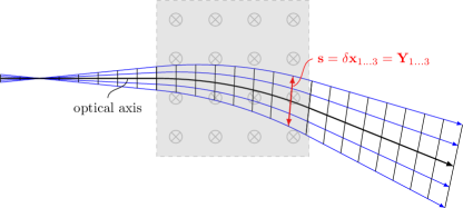
Figure 1: Paraxial trajectories in a constant transverse magnetic field of a magnetic deflector with sharp cut-offs. The thick red arrows denote the spatial deviation $\boldsymbol{s}\coloneqq\delta\boldsymbol{x}_{1\ldots 3}=\boldsymbol{Y}_{1\ldots 3}$ from the black reference trajectory (optical axis). Note that both transversal and longitudinal deviations to the reference trajectory are present in this example.

We now introduce the notion of the Lie derivative (see Appendix A) by defining the path deviation vector $\boldsymbol{Y}\coloneqq\delta\boldsymbol{x}$, which allows to reexpress the JVE (9) as a disappearance of the Lie derivative of the deviation vector $\boldsymbol{Y}$ along the optical axis (defined by vector field $\boldsymbol{X}$) $\mathcal{L}_{\boldsymbol{X}}\boldsymbol{Y}=0$ (see Appendix A). In other words, the deviation vectors $\boldsymbol{Y}$ form an invariant vector field along the optical axis, which has the following consequence. Inserting any two invariant vector fields $\boldsymbol{Y}$, $\boldsymbol{Z}$ (trajectories) as arguments into Liouville’s theorem yields

$$0=\mathcal{L}_{\boldsymbol{X}}\omega\left(\boldsymbol{Y},\boldsymbol{Z}\right)=\frac{d}{dt}\left[\omega\left(\boldsymbol{Y},\boldsymbol{Z}\right)\right]\,,$$ (10)

meaning that the phase space area spanned by $\boldsymbol{Y}$ and $\boldsymbol{Z}$ (measured by the Poincare 2-form $\omega$) along the optical axis is preserved. The conservation of transverse phase space areas (i.e., $\boldsymbol{Y}_{\bot}$and $\boldsymbol{Z}_{\bot}$ perpendicular to optical axis) in the object and image plane of anastigmatic optical elements (e.g., round lens) is referred to as the Lagrange-Helmholtz invariant. Similar Lagrange invariants follow for other elements such as energy filters (see Fig. 1 for an energy-dispersive deflector). From now on we shall always consider CPO as the transport of some (deviation) vector along the optical axis.

Inserting the Hamiltonian vector field (4) into (9), we obtain the coordinate expression for deviation vector motion in phase space

$$\frac{dY_{i}}{dt} =\chi_{ij}Y_{j}$$ (11)

$$=\frac{q}{m}\left(\begin{array}[]{c|c}-\frac{\partial A_{i}}{\partial r_{j}}&\frac{1}{q}\delta_{ij-3}\\ \hline\cr\frac{\partial^{2}A_{k}}{\partial r_{i-3}\partial r_{j}}\left(p_{k}-qA_{k}\right)-q\frac{\partial A_{k}}{\partial r_{i-3}}\frac{\partial A_{k}}{\partial r_{j}}-m\frac{\partial^{2}\Phi}{\partial r_{i-3}\partial r_{j}}&\frac{\partial A_{j-3}}{\partial r_{i-3}}\end{array}\right)_{\boldsymbol{x}\left(t\right)}Y_{j}$$ (14)

We can readily verify that $J\chi$ with the skew-symmetric $6\times 6$ matrix ($I_{3}$ denotes the $3\times 3$ identity matrix)

$$J=\begin{bmatrix}0&I_{3}\\ -I_{3}&0\end{bmatrix}$$ (15)

is symmetric, which is the defining property for a Hamiltonian matrix that form the symplectic Lie algebra $\mathrm{\boldsymbol{sp}}\left(6,\mathbb{R}\right)$. The corresponding exponential map including multiplications generate the symplectic group $\mathrm{Sp}\left(6,\mathbb{R}\right)$, which is another way of saying that deviation vectors governed by the JVE preserve phase space areas (see further below).

The above Lie derivative of a deviation vector in phase space is not gauge invariant. The equations of motion of the position vector ($\boldsymbol{s}=\boldsymbol{Y}_{1\ldots 3}$) derived by a second derivation of the first three entries of (11)

$$m\frac{d^{2}s_{i}}{dt^{2}} =-q\frac{\partial A_{i}}{\partial r_{j}}\frac{ds_{j}}{dt}-q\frac{\partial^{2}A_{i}}{\partial r_{j}\partial r_{k}}\frac{dr_{k}}{dt}s_{j}+\frac{dY_{i+3}}{dt}$$ (16)

$$=-qF_{ij}\frac{ds_{j}}{dt}-q\frac{\partial F_{ij}}{\partial r_{j}}\frac{dr_{k}}{dt}s_{j}+q\frac{\partial E_{i}}{\partial r_{j}}s_{j}\,,$$

however, contain only physical fields, i.e., the electric field $\boldsymbol{E}$ and the magnetic fields $\boldsymbol{B}$ (the latter as spatial components of the electromagnetic tensor $\boldsymbol{F}$) which are gauge invariant. In systems with straight optical axis, the transverse part (perpendicular to the optical axis) of these equations of motion are consistent with the usual paraxial approximation of the trajectory method derived from truncating the mulitpolar expansion of the electromagnetic fields around the optical axis to linear terms (e.g., [4]) with one notable exception: Being explicitly constructed as differences to a design trajectory the above paraxial equations do not contain any axial acceleration potential as this is already absorbed into the reference trajectory (i.e., optical axis).

The above JVE (11) and the ensuing paraxial Newtonian equations of motion (16) treat both transversal and longitudinal deviations as well as straight and curvilinear systems on the same footing. Both describe paraxial optics completely and can be efficiently solved by numerical (step) solvers, which is the standard procedure, if the electric and magnetic fields vary along the optical axis. Solving the second order differential equation (16) does not warrant gauge considerations and requires several integrations to obtain all fundamental solutions completely describing a given system. Integrating the JVE, on the other hand, directly yields the transfer matrix from one plane to another, however, gauge needs to be considered generally (see below). The latter argument may be turned around, however, as gauge freedom can be sometimes exploited (A) to simplify the solution of the coupled systems of first-order differential equations (11) and (B) to simplify the relation between kinetic and canonical momentum in particular planes of interest (e.g., object and image plane). One particular useful trick is to fix the gauge such to render $\chi\left(t\right)$ time-independent (i.e., constant along the optical axis), which leads to a particularly simple integration of (11). Moreover, conservation of phase space is an additional structure available in the JVE, which can be incorporated into efficient approximation schemes (i.e., geometrical integration, see below). These arguments carry over to the perturbation schemes rooted either in Newtonian equations of motion (i.e.the trajectory method) or Hamiltonian (next section) and Hamilton-Jacobi mechanics (i.e. the Lie algebra method).

To illustrate these aspects and to further the analytical treatment of the paraxial and higher order trajectory equations we elaborate on the solution of the JVE in the following. The formal solution to Eq. (11) is obtained by the time-ordered (symplectic) exponential map

$$Y_{i}\left(t\right)=\underset{\mathcal{M}_{ij}}{\underbrace{\mathcal{T}\exp\left\{\int_{0}^{t}\chi_{ij}\left(t_{1}\right)\differential t_{1}\right\}}}Y_{j}\left(0\right)\,,$$ (17)

where $\mathcal{T}$ is the time ordering operator. Thereby, the defined matrix $\mathcal{M}$ allows to compute the deviation vector $\boldsymbol{Y}\left(t\left(l\right)\right)$ of some trajectory at some time, defined by the arc length $l=\int_{0}^{t}v_{0}\left(t_{1}\right)\differential t_{1}$ of the optical axis given its initial phase space coordinates $\boldsymbol{Y}\left(0\right)$. As $\mathcal{M}$ is symplectic its inverse can be readily obtained from $\mathcal{M}^{-1}=-J\mathcal{M}^{T}J$, which is again in the symplectic group $\mathrm{Sp}\left(6,\mathbb{R}\right)$. We will see further below that the last property is a key to a straightforward evaluation of aberrations.

Here it is important to note that the locus of the spatial part of $\boldsymbol{Y}\left(t\right)$ at some fixed time $t$ is typically not confined to a single (image) plane even if we restrict the spatial part of $\boldsymbol{Y}\left(0\right)$ to a plane (i.e., all trajectories start in some (object) plane, see Fig. 1 for an example). In other words, there generally is a spatial longitudinal deviation between the spatial end point of the deviation vector and some predefined image plane intersected by the optical axis at $l$ (which is often but not necessarily perpendicular to the optical axis). This in turn leads to a positive or negative time lag $\delta t$ for the corresponding trajectory to reach the image plane, which is of first order in (i.e., depends linearly on) the initial deviation vector $\boldsymbol{Y}\left(0\right)$ of the trajectory. This leads to additional first order transversal deviations $\boldsymbol{Y}^{\left(t\right)}$ in the image plane that must be considered in the paraxial limit, if a non-zero deviation vector is produced by the additional time required to propagate the particle along the optical axis to the image plane, i.e.,

$$\boldsymbol{Y}^{\left(t\right)}\left(t\right)\approx\boldsymbol{X}_{\left(t\right)}\delta t\,.$$ (18)

Higher order propagation effects (i.e., stemming from the additional propagation of the deviation vector via $\mathcal{M}\left(\delta t\right)$ in (17)), on the other hand, may be neglected in the paraxial regime because these would be totally of second order in the initial beam coordinates as the time lag itself is already of first order. Consequently, the additional correction due to longitudinal deviations is important only when considering final planes located at a curved optical axis and we discuss one particular example, the sector magnet, in Appendix B.4. Note, however, that this correction vanishes, if image planes outside of the fields are considered. Here, the longitudinal transport along the optical axis does not introduce any additional first order effects as the zeroth order trajectory (optical axis) is straight and hence $\boldsymbol{Y}{}_{xy}^{\left(t\right)}\left(t\right)=0$. This condition can be also achieved “artificially” by rectifying a curved optical axis in curvilinear coordinates, which is the key argument for their use in literature. Here, we argue, however, that the paraxial time lag correction (18), if necessary at all (i.e., if considering planes at bend sections of the optical axis), is easy to compute, hence not increasing complexity in comparison to those coming with curvilinear coordinates.

In case of elements with straight optical axis, the transverse subspace of $\mathcal{M}$ corresponds to the transfer matrices of paraxial optics if $\boldsymbol{A}_{\perp}=0$ in the initial and final plane. Occasionally, gauge freedom can be exploited to achieve that condition. In the general case, however, a transformation $\mathcal{G}$ sending kinetic to canonical momentum

$$\mathcal{G} :\delta\boldsymbol{p}\left(t\right)\rightarrow m\delta\boldsymbol{v}\left(t\right)=\mathcal{G}\left(t\right)\circ\delta\boldsymbol{p}\left(t\right),$$ (19)

$$M\rightarrow M=\mathcal{G}\left(t\right)\circ\mathcal{M}\circ\mathcal{G}^{-1}\left(0\right)$$

is required ($\circ$ denotes the application of that transformation) to obtain the gauge invariant transfer matrix for configurations space (i.e., consisting of $\boldsymbol{r}$ and kinetic momentum)

$$\boldsymbol{Y}^{\mathrm{kin}}\left(t\right)=M\boldsymbol{Y}^{\mathrm{kin}}\left(0\right)\,.$$ (20)

A particular simple situation is encountered if $\mathcal{G}$ is linear in the position vector, i.e,. may be represented by a matrix $G$ (see discussion of the Wien filter in Appendix B for an example)

$$M=G\left(t\right)\mathcal{M}G^{-1}\left(0\right)\,.$$ (21)

Eq. (17) generally does not admit closed expressions for the transfer matrix and requires using numerical integrators (e.g., directly applied to (11)). Note, however, that closed solutions exist for a number of special cases; moreover, series expansions may be used to obtain analytical approximations of increasing accuracy. Solving (17) is straightforward if $\chi\left(t\right)$ commutate for all times $t$ (which includes time-independent $\chi$), yielding

$$\mathcal{M} =\exp\left(\int_{0}^{t}\chi\left(t_{1}\right)\differential t_{1}\right)\,.$$ (22)

Indeed, increasingly better approximation to general transfer matrices may be obtained from the Magnus expansion[15]

$${\displaystyle\mathcal{M}=\exp\left(\sum_{k=1}^{\infty}\Omega_{k}\right)\,,}$$ (23)

with the first two terms ($k=1,2$) explicitly reading

$$\Omega_{1}(t) =\int_{0}^{t}\chi(t_{1})\differential t_{1}$$ (24)

$$\Omega_{2}(t) =\frac{1}{2}\int_{0}^{t}\differential t_{1}\int_{0}^{t_{1}}\differential t_{2}[\chi(t_{1}),\chi(t_{2})]\,.$$

Here, $\left[\cdot,\cdot\right]$ denotes the commutator. Notably, the Magnus expansion conserves phase space and hence Lagrange invariants at every order of the approximation (i.e., truncation of (23)), a property that is not shared by the class of multistep integrators or Runge-Kutta methods. In other words, it falls in the class of geometric integrators[16], rendering it a useful tool to describe the paraxial optics of general systems with fields varying along the optical axis (see discussion of the round lens in Appendix B for an exemplary application of Magnus expansion).

We finally also note the fully relativistic expressions for the Hamiltonian vector field

$$\boldsymbol{X} =\begin{pmatrix}{\displaystyle\frac{\mathbf{p}-q\mathbf{A}}{\sqrt{m^{2}+\frac{1}{c^{2}}\left(\mathbf{p}-q\mathbf{A}\right)^{2}}}}\\ {\displaystyle q\frac{\partial A^{i}}{\partial\boldsymbol{r}}{\displaystyle\frac{p_{i}-qA_{i}}{\sqrt{m^{2}+\frac{1}{c^{2}}\left(\mathbf{p}-q\mathbf{A}\right)^{2}}}}-q\frac{\partial\Phi}{\partial\boldsymbol{r}}}\end{pmatrix}$$ (25)

$$=\begin{pmatrix}{\displaystyle\frac{\mathbf{p}-q\mathbf{A}}{\gamma m}}\\ {\displaystyle q\frac{\partial A_{i}}{\partial\boldsymbol{r}}{\displaystyle\frac{p_{i}-qA_{i}}{\gamma m}}-q\frac{\partial\Phi}{\partial\boldsymbol{r}}}\end{pmatrix}\,,$$

and the ensuing JVE

$$\frac{dY_{i}}{dt}=\frac{q}{\gamma m}\left(\begin{array}[]{c|c}-\frac{\partial A_{i}}{\partial r_{j}}+\frac{\partial A_{k}}{\partial r_{j}}\frac{p_{k}-qA_{k}}{c^{2}\left(\gamma m\right)^{2}}\left(p_{i}-qA_{i}\right)&\frac{1}{q}\left(\delta_{ij-3}-\frac{\left(p_{i}-qA_{i}\right)\left(p_{j-3}-qA_{j-3}\right)}{c^{2}\left(\gamma m\right)^{2}}\right)\\ \hline\cr\begin{array}[]{c}\frac{\partial^{2}A_{k}}{\partial r^{j}\partial r_{i-3}}{\displaystyle\left(p_{k}-qA_{k}\right)}-\frac{\partial A_{k}}{\partial r_{i-3}}\frac{\partial A_{k}}{\partial r_{j}}\\ +\frac{\partial A_{k}}{\partial r_{i-3}}\left(p_{k}-qA_{k}\right)\frac{\partial A_{l}}{\partial r_{j}}{\displaystyle\frac{p_{l}-qA_{l}}{c^{2}\left(\gamma m\right)^{2}}}-\gamma m\frac{\partial^{2}\Phi}{\partial r_{i-3}\partial r_{j}}\end{array}&\frac{\partial A_{j-3}}{\partial r_{i-3}}-\frac{\partial A_{k}}{\partial r_{i-3}}\frac{p_{k}-qA_{k}}{c^{2}\left(\gamma m\right)^{2}}\left(p_{j}-qA_{j}\right)\end{array}\right)_{\boldsymbol{x}\left(t\right)}Y_{j}\,.$$ (26)

The latter considerably simplifies if we consider optical elements, where the kinetic energy of the particles is conserved (i.e., all purely magnetic elements)

$$\frac{dY_{i}}{dt}=\frac{q}{\gamma m}\left(\begin{array}[]{c|c}-\frac{\partial A_{i}}{\partial r_{j}}&\frac{1}{q}\delta_{ij-3}\\ \hline\cr\frac{\partial^{2}A_{k}}{\partial r_{i-3}\partial r_{j}}\left(p_{k}-qA_{k}\right)-q\frac{\partial A_{k}}{\partial r_{i-3}}\frac{\partial A_{k}}{\partial r_{j}}-\gamma m\frac{\partial^{2}\Phi}{\partial r_{i-3}\partial r_{j}}&\frac{\partial A_{j-3}}{\partial r_{i-3}}\end{array}\right)_{\boldsymbol{x}\left(t\right)}Y_{j}\,.$$ (27)

Accordingly, we only have to replace $m\rightarrow\gamma m$ in the non-relativistic second order paraxial equations of motion in this case

$$\gamma m\frac{d^{2}s_{i}}{dt^{2}}=-qF_{ij}\frac{ds_{j}}{dt}-q\frac{\partial F_{ij}}{\partial r_{j}}\frac{dr_{k}}{dt}s_{j}\,.$$ (28)

The simplified relativistic JVE covers a wide range of CPO devices since electric components are seldom employed at relativistic energies, as their deflection efficiency falls with the beam energy.

In the Appendix we will describe a set of non-relativistic or purely magnetic examples of elementary CPO devices using the previously developed framework: the magnetic quadrupole, the magnetic round lens, the Wien filter and the magnetic sector magnet. Here, we put the main focus on illustrating the several computation steps, notably including gauge, Magnus expansion and curved systems.

IV Aberration Theory

The iterative computation of higher order aberrations begins with collecting quadratic terms ($n=2$) of $\varepsilon$ in (8), corresponding to the first order aberration level. One obtains the following coupled system of inhomogeneous first order differential equations

$$\frac{d\left(Y_{i}^{\left(2\right)}\right)}{dt}=\left(\frac{\partial X_{i}}{\partial x_{j}}\right)_{\boldsymbol{x}\left(t\right)}Y_{j}^{\left(2\right)}+\frac{1}{2}\left(\frac{\partial^{2}X_{i}}{\partial x_{j_{1}}\partial x_{j_{2}}}\right)_{\boldsymbol{x}\left(t\right)}Y_{j_{1}}^{\left(1\right)}Y_{j_{2}}^{\left(1\right)}\,,$$ (29)

which define the first order aberrations (see below). Noting that $Y_{i}^{\left(2\right)}\left(0\right)=0$ (i.e., starting conditions have been absorbed by paraxial trajectory) the solution of such a first order matrix differential equation can be formally written as

$$Y_{i}^{\left(2\right)}\left(t\right) =\frac{1}{2}\mathcal{M}_{ij}\left(t\right)\int_{0}^{t}\mathcal{M}_{jk}^{-1}\left(t_{1}\right)\left(\frac{\partial^{2}X_{k}}{\partial x_{j_{1}}\partial x_{j_{2}}}\right)_{\boldsymbol{x}\left(t_{1}\right)}Y_{j_{1}}^{\left(1\right)}\left(t_{1}\right)Y_{j_{2}}^{\left(1\right)}\left(t_{1}\right)\differential t_{1}$$ (30)

$$=\underset{\mathcal{M}_{il_{1}l_{2}}^{\left(2\right)}}{\underbrace{\left(\frac{1}{2}\mathcal{M}_{ij}\left(t\right)\int_{0}^{t}\left(J^{T}\mathcal{M}^{T}J\right)_{jk}\left(t_{1}\right)\left(\frac{\partial^{2}X_{k}}{\partial x_{j_{1}}\partial x_{j_{2}}}\right)_{\boldsymbol{x}\left(t_{1}\right)}\mathcal{M}_{j_{1}l_{1}}\left(t_{1}\right)\mathcal{M}_{j_{2}l_{2}}\left(t_{1}\right)\differential t_{1}\right)}}Y_{l_{1}}\left(0\right)Y_{l_{2}}\left(0\right)\,,$$

where $\mathcal{M}$ denotes the paraxial transfer matrices (17) as usual. On the second line, we exploited the inversion formula for symplectic matrices noted previously. The form of the solution reveals the second order polynomial dependency of the second order path deviation from the the initial path phase space coordinates. Accordingly, we denote the second order “transfer matrix” (indeed a vector-valued 2-form) by $\mathcal{M}^{\left(2\right)}$.

Inspecting the definition of $\mathcal{M}^{\left(2\right)}$, we observe that it is symmetric in the last two indices. Another set of fundamental symmetries follows from the Jacobian of the Hamiltonian flow being a Hamiltonian matrix and the Gaussian transfer matrices being symplectic, ultimately leading to interdependencies between aberrations. Additional restrictions may hold if the optical system has certain symmetries, which restrict the non-zero entries of the derivatives of the Jacobian of the Hamiltonian flow. Abstractly, they may be also derived from symmetry conditions $\mathcal{M}^{\left(2\right)}=S\mathcal{M}^{\left(2\right)}S^{-1}S^{-1},$where the matrices $S$ are representations of some symmetry operation and operate on one particular index of $\mathcal{M}$ in the given order. Another set of restrictions is imposed, when considering particular pairs of planes, where the paraxial transfer matrices assume a particular simple shape. E.g., in case of stigmatic imaging

$$\mathcal{M}\left(t\right)=\left(\begin{array}[]{c|c}A&0\\ \hline\cr B&A^{-1}\end{array}\right)$$ (31)

with $3\times 3$ block matrices $A$ and $B$. To bring the above integral to an analytically more tractable form one may finally apply further approximations, such as the first order Magnus approximation, i.e., $\mathcal{M}\approx\exp\left(\int\chi dt\right)$, or the weak field approximation, i.e., $\mathcal{M}\approx 1+\int\chi dt$, if appropriate.

Further insight into the properties of (second order) path deviations can be obtained by considering phase space areas spanned by deviation vectors. To see that we first note that the directional derivative along the Hamiltonian flow of the phase space areas spanned by $\boldsymbol{Y}^{\left(1\right)}+\boldsymbol{Y}^{\left(2\right)}$ and a Gaussian reference trajectory $\boldsymbol{Z}^{\left(1\right)}$ reads (see AppendixA)

$$\boldsymbol{X}\left\{\omega\left(\boldsymbol{Y}^{\left(1\right)}+\boldsymbol{Y}^{\left(2\right)},\boldsymbol{Z}^{\left(1\right)}\right)\right\}=\omega\left(\mathcal{L}_{\boldsymbol{X}}\boldsymbol{Y}^{\left(2\right)},\boldsymbol{Z}^{\left(1\right)}\right)$$ (32)

Inserting (29) and pulling back to the design trajectory parameterization $t$ then gives

$$\derivative{t}\left[\omega\left(\boldsymbol{Y}^{\left(1\right)}+\boldsymbol{Y}^{\left(2\right)},\boldsymbol{Z}^{\left(1\right)}\right)\right]=\frac{1}{2}\omega\left(\left(\frac{\partial^{2}\boldsymbol{X}}{\partial x_{j_{1}}\partial x_{j_{2}}}\right)_{\boldsymbol{x}\left(t\right)}Y_{j_{1}}^{\left(1\right)}Y_{j_{2}}^{\left(1\right)},\boldsymbol{Z}^{\left(1\right)}\right)\,.$$ (33)

This differential equation may be directly integrated taking into account $\boldsymbol{Y}^{\left(2\right)}\left(t_{i}\right)=0$ yielding

$$\omega\left(\boldsymbol{Y}^{\left(1\right)}+\boldsymbol{Y}^{\left(2\right)},\boldsymbol{Z}^{\left(1\right)},t\right)-\omega\left(\boldsymbol{Y}^{\left(1\right)},\boldsymbol{Z}^{\left(1\right)},0\right)=\omega\left(\boldsymbol{Y}^{\left(2\right)},\boldsymbol{Z}^{\left(1\right)},t\right)=\frac{1}{2}\int_{0}^{t}\omega\left(\left(\frac{\partial^{2}\boldsymbol{X}}{\partial x_{j_{1}}\partial x_{j_{2}}}\right)_{\boldsymbol{x}\left(t\right)}Y_{j_{1}}^{\left(1\right)}Y\left(t_{1}\right)_{j_{2}}^{\left(1\right)}\left(t_{1}\right),\boldsymbol{Z}^{\left(1\right)}\left(t_{1}\right)\right)\differential t_{1}$$ (34)

These relations replace the Lagrange invariants of the paraxial case, based on $\derivative{t}\left[\omega\left(\boldsymbol{Y}^{\left(1\right)},\boldsymbol{Z}^{\left(1\right)}\right)\right]=0$. Indeed, (34) correspond to the expressions evaluated in the so-called eikonal methods (e.g., [4]). The latter essentially solve (34) for maximally six (often fewer are sufficient) linearly independent referenze trajectories $\boldsymbol{Z}_{1..6}^{\left(1\right)}$, which allows to determine all six components of $\boldsymbol{Y}^{\left(2\right)}$by solving the 6 equations $\omega\left(\boldsymbol{Y}^{\left(2\right)},\boldsymbol{Z}_{1..6}^{\left(1\right)},t\right)$ for $\boldsymbol{Y}^{\left(2\right)}$. The latter is always possible as the two-form $\omega$ is non-degenerate. Note, furthermore, that the Gaussian reference trajectories $\boldsymbol{Z}^{\left(1\right)}$ may be in principle chosen such to coincide with the second order trajectory $\boldsymbol{Y}^{\left(1\right)}+\boldsymbol{Y}^{\left(2\right)}$ in only one phase space coordinate (either position or momentum) in the initial plane and another one in the final plane (or any other, such a the aperture plane), respectively. The evaluation of (34) using such mixed boundary conditions is, however, not straight forward as the value of $\boldsymbol{Y}^{\left(2\right)}$ at the second plane is only implicitely defined.

We finally have to consider two important aspects of the above aberration theory: (A) Additional set of deviations introduced by the longitudinal position deviations with respect to some predefined final plane (e.g., image plane). The longitudinal deviations correspond to a time lag for the particle to reach the final plane which can lead to additional aberrations after propagation to that plane. (B) The canonical momentum deviation considered above needs to be transformed into kinetic momentum to obtain experimentally observable quantities. We simplify both considerations by discussing initial and final planes, which are outside of the fields of the optical elements (constant non-zero potentials remain possible). That is a minor restriction considering that we are mostly interested into the properties of optical elements with respect to planes lying outside. Notable exceptions are, for instance, the asymptotic properties of objective lenses in a transmission electron microscope, where the object plane is immersed in the magnetic field. Under these prerequisites the trajectories in the initial and final plane are straight and kinetic and canonical momentum are equivalent. Consequently, we only have to add a first order correction due to transit time differences $\delta t$ to some predefined final plane, reading

$$Y_{i}{}^{\left(2t\right)}\left(t\right) \approx-\chi_{ij}\left(t\right)Y_{j}^{\left(1\right)}\left(t\right)\delta t$$ (35)

$$=-\frac{1}{mv}\left(\begin{array}[]{c|c}0&I_{3}\\ \hline\cr 0&0\end{array}\right)_{ij}Y_{j}^{\left(1\right)}\left(t\right)Y_{3}^{\left(1\right)}\left(t\right)$$ (38)

$$=\underset{\mathcal{M}_{il_{1}l_{2}}^{\left(2t\right)}}{\underbrace{-\frac{1}{mv}\left(\begin{array}[]{c|c}0&I_{3}\\ \hline\cr 0&0\end{array}\right)_{ij}\mathcal{M}_{jl_{1}}\mathcal{M}_{3l_{2}}}}Y_{l_{1}}\left(0\right)Y_{l_{2}}\left(0\right)\,,$$ (41)

where the explicit form of the free space Jacobian of the Hamiltonian flow has been inserted. It is furthermore useful to symmetrize $\mathcal{M}^{\left(2t\right)}$ in the last two indices as there is no preferred choice, i.e., $\mathcal{M}_{il_{1}l_{2}}^{\left(2t\right)}=\nicefrac{{\left(\mathcal{M}_{il_{1}l_{2}}^{\left(2t\right)}+\mathcal{M}_{il_{2}l_{1}}^{\left(2t\right)}\right)}}{{2}}$. In order to obtain aberration coefficients, which we define here as the dependency of path deviations of a certain order in some final plane on homogeneous polynomials of corresponding order (here 2) of position and kinetic momentum in some initial plane, we finally have to add the above two contributions, i.e., $C_{ijj}^{\left(2\right)}=M_{ijj}^{\left(2\right)}+M_{ijj}^{\left(2t\right)}$ and $C_{ijk\neq j}^{\left(2\right)}=2\left(M_{ijk}^{\left(2\right)}+M_{ijk}^{\left(2t\right)}\right)$, where the factor 2 accounts for the combinatorial multiplicity of the two symmetric terms in $M^{\left(2\right)}$.

The above sketched program may now be extended to higher order aberrations with little modifications: The inhomogeneous system of first order differential equations defining the third order path deviations in phase space read

$$\derivative{Y_{i}^{\left(3\right)}}{t}\approx\left(\frac{\partial X_{i}}{\partial x_{j}}\right)_{\boldsymbol{x}\left(t\right)}Y_{j}^{\left(3\right)}+\left(\frac{\partial^{2}X_{i}}{\partial x_{j_{1}}\partial x_{j_{2}}}\right)_{\boldsymbol{x}\left(t\right)}Y_{j_{1}}^{\left(1\right)}Y_{j_{2}}^{\left(2\right)}+\frac{1}{6}\left(\frac{\partial^{3}X_{i}}{\partial x_{j_{1}}\partial x_{j_{2}}\partial x_{j_{3}}}\right)_{\boldsymbol{x}\left(t\right)}Y_{j_{1}}^{\left(1\right)}Y_{j_{2}}^{\left(1\right)}Y_{j_{3}}^{\left(1\right)}\,.$$ (42)

Again solutions can be obtained by direct integration

$$Y_{i}^{\left(3\right)}\left(t\right) =\mathcal{M}_{ij}\left(t\right)\int_{0}^{t}\left(J^{T}\mathcal{M}^{T}J\right)_{jk}\left(t_{1}\right)\left(\left(\frac{\partial^{2}X_{k}}{\partial x_{j_{1}}\partial x_{j_{2}}}\right)_{\boldsymbol{x}\left(t_{1}\right)}Y_{j_{1}}^{\left(1\right)}\left(t_{1}\right)Y_{j_{2}}^{\left(2\right)}\left(t_{1}\right)\right.$$ (43)

$$+\left.\frac{1}{6}\left(\frac{\partial^{2}X_{k}}{\partial x_{j_{1}}\partial x_{j_{2}}x_{j_{1}}\partial x_{j_{3}}}\right)_{\boldsymbol{x}\left(t_{1}\right)}Y_{j_{1}}^{\left(1\right)}\left(t_{1}\right)Y_{j_{2}}^{\left(1\right)}\left(t_{1}\right)Y_{j_{3}}^{\left(1\right)}\left(t_{1}\right)\right)\differential t_{1}$$

$$=\left(\mathcal{M}_{ij}\left(t\right)\int_{0}^{t}\left(J^{T}\mathcal{M}^{T}J\right)_{jk}\left(t_{1}\right)\left(\frac{\partial^{2}X_{k}}{\partial x_{j_{1}}\partial x_{j_{2}}}\right)_{\boldsymbol{x}\left(t_{1}\right)}\mathcal{M}_{j_{1}l_{1}}\left(t_{1}\right)\mathcal{M}_{j_{2}l_{2}l_{3}}^{\left(2\right)}\left(t_{1}\right)\differential t_{1}\right.$$

$$+\left.\frac{1}{6}\mathcal{M}_{ij}\left(t\right)\int_{0}^{t}\left(J^{T}\mathcal{M}^{T}J\right)_{jk}\left(t_{1}\right)\left(\frac{\partial^{2}X_{k}}{\partial x_{j_{1}}\partial x_{j_{2}}x_{j_{1}}\partial x_{j_{3}}}\right)_{\boldsymbol{x}\left(t_{1}\right)}\mathcal{M}_{j_{1}l_{1}}\left(t_{1}\right)\mathcal{M}_{j_{2}l_{2}}\left(t_{1}\right)\mathcal{M}_{j_{3}l_{3}}\left(t_{1}\right)\differential t_{1}\right)Y_{l_{1}}^{\left(1\right)}\left(0\right)Y_{l_{2}}^{\left(1\right)}\left(0\right)Y_{l_{3}}^{\left(1\right)}\left(0\right)\,.$$

The expression on the third line may be further symmetrized with respect to $l_{1...3}$ as there is no preferred choice in the ordering of the corresponding $\boldsymbol{Y}_{l_{1...3}}\left(0\right)$. Again, the whole prefactor of the third order polynomial of initial beam parameters can be referred to as generalized transfer matrix $\mathcal{M}^{\left(3\right)}$. Additional corrections due to transit time lags (taking into account that derivatives of $\chi$ in vacuum are zero) read

$$\boldsymbol{Y}^{\left(3t\right)}\left(t\right) \approx-\frac{1}{m}\left(\begin{array}[]{c|c}0&I_{3}\\ \hline\cr 0&0\end{array}\right)\boldsymbol{Y}^{\left(1\right)}\left(t\right)\delta t^{\left(2\right)}$$ (46)

$$=-\frac{1}{mv}\left(\begin{array}[]{c|c}0&I_{3}\\ \hline\cr 0&0\end{array}\right)_{ij}Y_{j}^{\left(1\right)}\left(t\right)Y_{3}^{\left(2\right)}\left(t\right)$$ (49)

$$=\underset{\mathcal{M}_{il_{1}l_{2}l_{3}}^{\left(3t\right)}}{\underbrace{-\frac{1}{mv}\left(\begin{array}[]{c|c}0&I_{3}\\ \hline\cr 0&0\end{array}\right)_{ij}\mathcal{M}_{jl_{1}}\mathcal{M}_{3l_{2}l_{3}}^{\left(2\right)}}}Y_{l_{1}}^{\left(1\right)}\left(0\right)Y_{l_{2}}^{\left(1\right)}\left(0\right)Y_{l_{3}}^{\left(1\right)}\left(0\right)\,.$$ (52)

Again, the unsymmetrized expression is shown. Note, that a technical complication in the above expressions is given by the presence of second order deviations $Y_{j_{2}}^{\left(2\right)}$ in the integral in the first line of (43) and the second line of (46). These terms are sometimes referred to as intrinsic combination aberrations (as lower order combine to higher order aberrations), and can be calculated with the help of (30), leading, e.g., to the double integrals on the third line of (43). The third and higher aberration orders (i.e., $\boldsymbol{Y}^{\left(n>3\right)}$deviation vectors) can be derived exactly along the same lines. In Appendix B we will discuss the first order aberrations of the quadrupole and Wien filter illustrating the above framework.

V Discussion and Outlook

To sum up, an exhaustive yet compact description of charged particle optics rooted in Hamiltonian mechanics has been presented. The main features are incorporation of transversal and longitudinal (i.e., chromatic) path deviations in static and time-dependent fields on the same footing, a unified and simple description of both straight and curved systems, the straightforward computation of transfer matrices up to any perturbation order (i.e., aberrations), and an efficient geometric integration scheme. The framework shall be useful for characterization of general CPO devices with regard to two aspects: (A) Employing closed analytical approximations for the paraxial transfer matrices $M$ derived from the Magnus expansion allows to write down analytical expressions for the aberration coefficients. Notwithstanding their approximate character such expressions are useful to quickly evaluate the importance of certain aberrations and possible reduction strategies. (B) Employing “exact” paraxial transfer matrices (either obtained by multi-step methods or geometric integrators) the aberration integrals may be efficiently integrated numerically, yielding fast and accurate perturbative trajectory solvers.

VI Acknowledgement

We are deeply indebted to Stephan Uhlemann, Heiko Müller and Peter Hawkes for invaluable discussions and comments. We furthermore acknowledge funding from the European Research Council (ERC) under the Horizon 2020 research and innovation program of the European Union (grant agreement no. 715620).

VII Bibliogaphy

Appendix A Lie Derivative

This section introduces the notion of the Lie derivative as employed in the main text. The notation is adapted from [13], which also contains a comprehensive introduction into the topic. The Lie derivative of a vector field is defined as

$${\displaystyle(\mathcal{L}_{\boldsymbol{X}}\boldsymbol{Y})_{\boldsymbol{x}}=\left.\frac{d}{dt}\right|_{t=0}\left((\varphi_{-t})_{*}\boldsymbol{Y}_{\varphi_{t}(\boldsymbol{x})}\right).}$$ (53)

Here, the 1-parameter group (flow) $\varphi$ is given by

$$\frac{d}{dt}\varphi=\boldsymbol{X}$$ (54)

and $\varphi{}_{*}$ denotes its differential. For our purposes $\boldsymbol{Y}$ needs to be defined along the flow generated by $\boldsymbol{X}$only (which corresponds to the optical axis). The coordinate expression for the Lie derivative reads

$$\left(\mathcal{L}_{\boldsymbol{X}}\boldsymbol{Y}\right)_{i} =\frac{\partial Y^{i}}{\partial x^{j}}X^{j}-\frac{\partial X_{i}}{\partial x_{j}}Y_{j}$$ (55)

$$=\frac{dY_{i}}{dt}-\frac{\partial X_{i}}{\partial x_{j}}Y_{j}\,.$$

In the main text we are concerned with so-called invariant vector fields fulfilling $\mathcal{L}_{\boldsymbol{X}}\boldsymbol{Y}=0$, for which the Lie derivative of a $p$-dimensional form evaluated on invariant vector fields $\boldsymbol{Y}$reads

$$\mathcal{L}_{\boldsymbol{X}}\omega^{p}\left(\boldsymbol{Y}_{1},\ldots,\boldsymbol{Y}_{p}\right)=\frac{d}{dt}\left[\omega_{\varphi_{t}x}^{p}\left(\boldsymbol{Y}_{1},\ldots,\boldsymbol{Y}_{p}\right)\right]\,.$$ (56)

Consequently, in our phase space setting, $\mathcal{L}_{\boldsymbol{X}}\omega\left(\boldsymbol{Y}_{1},\boldsymbol{Y}_{2}\right)$ measures the derivative, with respect to motion along the optical axis, of phase space areas spanned by vector fields $\boldsymbol{Y}$, which equates to zero according to Liouville’s theorem. Finally, from the “Leibniz” rule for the Lie derivative we can equate the directional derivative of the Poincare 2-form of arbitrary vector fields along the optical axis with Poincare 2-forms of Lie derivatives[13]

$$\boldsymbol{X}\left\{\omega\left(\boldsymbol{Y},\boldsymbol{Z}\right)\right\}=\omega\left(\mathcal{L}_{\boldsymbol{X}}\boldsymbol{Y},\boldsymbol{Z}\right)+\omega\left(\boldsymbol{Y},\mathcal{L}_{\boldsymbol{X}}\boldsymbol{Z}\right)\,.$$ (57)

Appendix B Examples

In this Appendix we illustrate the various working principles of the above framework at the example of four basic CPO elements, which are important in numerous applications: (A) the magnetic quadrupole, (B) the round magnetic lens, (C) the Wien filter, and (D) the sector magnet. The first three elements have a straight optical axis, whereas the sector magnet has a curved optical axis. The first two examples show no variation in the transverse trajectory coordinates with respect to an energy change in the paraxial limit. The last two shows a first order dispersion, because of which they are used in energy filters and monochromator applications. In the specific case of electron optics, the first, second and fourth are purely magnetic and typically operate with relativistic electrons, whereas the Wien filter typically resides, where the electrons are rather slow (non-relativistic). As the pure relativistic magnetic systems can be described by the simplified relativistic Hamiltonian flow (27), we implicitly assume relativistic masses and omit $\gamma$ in the following expressions.

The level of the discussion will vary from element to element to keep the length at bay while illustrating all important aspects. E.g., quadrupole and Wien filter contain evaluation of aberrations, which are omitted for the lens and sector magnet. The lens on the other hand is the only example in which the field varies with the optical axis. For the other three cases we will only consider homogeneous fields, which are sharply cut-off at the entrance and exit plane of the respective device (such a neglection of fringing fields does not adequately describes real elements, we will furthermore not elaborate on the implications of the sharp cut-off on aberrations). The sector magnet section mainly focusses on the implications of a curved optical axis. We generally keep the discussion of the final results short as they are typically well-known and our main goal is the illustration of the machinery developed in the manuscript.

B.1 Magnetic Quadrupole

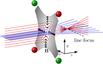
Figure 2: Paraxial optics of a thin quadrupole: Blue and red trajectories in the two principal planes are focused and defocused, respectively. Magnetic field lines illustrate the 45° rotation of the magnetic poles with respect to the two principal planes.

Magnetic quadrupoles are used as stigmators and anisotropic focusing elements in various CPO applications across the whole velocity range [17, 18]. They focus in one plane and defocus in the perpendicular one. The $\boldsymbol{B}$-field within the poles, rotated about 45° with respect to the coordinate system, can be described by linearly increasing Cartesian components (this expression is exact for hyperbolic poles; otherwise it is a good approximation close to the optical axis)

$$\boldsymbol{B}=-D_{2}\begin{pmatrix}y\\ x\\ 0\end{pmatrix}\,.$$ (58)

The vector potential in a Coulomb gauge ensuring z-independence reads

$$\boldsymbol{A}=\frac{1}{2}D_{2}\begin{pmatrix}0\\ 0\\ x^{2}-y^{2}\end{pmatrix}\,,$$ (59)

which leads to a time independent Jacobian in the JVE (11)

$$\chi=\left(\begin{array}[]{c|c}0&\begin{array}[]{ccc}\frac{1}{m}&0&0\\ 0&\frac{1}{m}&0\\ 0&0&\frac{1}{m}\end{array}\\ \hline\cr\begin{array}[]{ccc}qD_{2}v&0&0\\ 0&-qD_{2}v&0\\ 0&0&0\end{array}&0\end{array}\right)\,.$$ (60)

and no further implications from the sharp cut-off fields. Accordingly, the decoupling of the two principal planes is established at this stage with the $z$-direction being a trivial propagation. The exactly solvable transfer matrices for a quadrupole of length $l=vt$ in the defocusing and focusing plane then read

$$M_{x} =\exp\begin{pmatrix}0&\frac{l}{mv}\\ qD_{2}l&0\end{pmatrix}$$ (61)

$$=\begin{pmatrix}\mathrm{cosh}\left(kl\right)&\frac{1}{kp_{0}}\mathrm{sinh}\left(kl\right)\\ kp_{0}\mathrm{sinh}\left(kl\right)&\mathrm{cosh}\left(kl\right)\end{pmatrix}\,,$$

$$M_{y}=\begin{pmatrix}\mathrm{cos}\left(kl\right)&\frac{1}{kp_{0}}\mathrm{sin}\left(kl\right)\\ -kp_{0}\mathrm{sin}\left(kl\right)&\mathrm{cos}\left(kl\right)\end{pmatrix}\,,$$ (62)

and

$$M_{z}=\begin{pmatrix}1&\frac{l}{p_{0}}\\ 0&1\end{pmatrix}\,,$$ (63)

with $k=\sqrt{\frac{qD_{2}}{p_{0}}}$. These transfer matrices need not be corrected for the kinetic momentum since $A_{x}=A_{y}=0$ and hence they are exactly equal to those obtained from the solution of conventional paraxial theory [19, 6].

The first order aberrations follow from

$$\left(\frac{\partial X_{i}}{\partial x_{j}\partial x_{k}}\right)_{x\left(t\right)}=\frac{qD_{2}}{m}\left(\begin{array}[]{c|c}\begin{array}[]{ccc}-\delta_{i,3}&0&0\\ 0&\delta_{i,3}&0\\ 0&0&0\end{array}&\begin{array}[]{ccc}0&0&\delta_{i,4}\\ 0&0&-\delta_{i,5}\\ 0&0&0\end{array}\\ \hline\cr\begin{array}[]{ccc}0&0&0\\ 0&0&0\\ \delta_{i,4}&-\delta_{i,5}&0\end{array}&0\end{array}\right)$$ (64)

which leads to a second order transfer matrix $\mathcal{M}^{\left(2\right)}$ given by (30) with a few non-zero elements only. In case of the transverse elements these pertain to dependencies on the initial longitudinal momentum, i.e.,

$$\mathcal{M}_{116}^{\left(2\right)}=\mathcal{M}_{161}^{\left(2\right)} =\frac{kl\sinh\left(kl\right)}{4p_{0}}$$ (65)

$$\mathcal{M}_{146}^{\left(2\right)}=\mathcal{M}_{164}^{\left(2\right)} =\frac{kl\cosh\left(kl\right)-\sinh\left(kl\right)}{4kp_{0}^{2}}$$

$$\mathcal{M}_{226}^{\left(2\right)}=\mathcal{M}_{262}^{\left(2\right)} =-\frac{kl\sin\left(kl\right)}{4p_{0}}$$

$$\mathcal{M}_{256}^{\left(2\right)}=\mathcal{M}_{265}^{\left(2\right)} =\frac{kl\cos\left(kl\right)-\sin\left(kl\right)}{4kp_{0}^{2}}$$

$$\mathcal{M}_{416}^{\left(2\right)}=\mathcal{M}_{461}^{\left(2\right)} =\frac{k\left(kl\cosh\left(kl\right)+\sinh\left(kl\right)\right)}{4}$$

$$\mathcal{M}_{446}^{\left(2\right)}=\mathcal{M}_{264}^{\left(2\right)} =\frac{kl\sinh\left(kl\right)}{4p_{0}}$$

$$\mathcal{M}_{526}^{\left(2\right)}=\mathcal{M}_{562}^{\left(2\right)} =-\frac{k\left(\sin\left(kl\right)+kl\cos\left(kl\right)\right)}{4}$$

$$\mathcal{M}_{556}^{\left(2\right)}=\mathcal{M}_{565}^{\left(2\right)} =-\frac{kl\sin\left(kl\right)}{4p_{0}}$$

The non-zero longitudinal deviation (i.e., $\mathcal{M}_{3..}^{\left(2\right)}$) can be omitted because it introduces no effective second order deviation in the image plane after time-lag correction. In order to obtain aberration coefficients, i.e., the overall dependency of the final deviation vector $\boldsymbol{Y}^{\left(2\right)}$ from (second order) polynomials in the initial coordinates, we have to sum the symmetric contributions, e.g., $C_{116}^{\left(2\right)}=M_{116}^{\left(2\right)}+M_{161}^{\left(2\right)}=2M_{116}^{\left(2\right)}$, and add time lag aberrations (35) to final plane perpendicular to optical axis

$$Y_{i}{}^{\left(2t\right)}\left(t\right)=-\frac{1}{p_{0}^{2}}\left(\begin{array}[]{c|c}0&I_{3}\\ \hline\cr 0&0\end{array}\right)_{ij}\mathcal{M}_{jl_{1}}Y_{l_{1}}\left(0\right)Y_{6}\left(0\right)\,,$$ (66)

which gives

$$C_{116}^{\left(t\right)} =-\frac{kl\sinh\left(kl\right)}{p_{0}}$$ (67)

$$C_{146}^{\left(t\right)} =-\frac{l\cosh\left(kl\right)}{p_{0}^{2}}$$

$$C_{226}^{\left(t\right)} =\frac{kl}{p_{0}}\sin\left(kl\right)$$

$$C_{256}^{\left(t\right)} =-\frac{l}{p_{0}^{2}}\cos(kl)$$

$$C_{366}^{\left(t\right)} =-\frac{l}{p_{0}^{2}}\,.$$

Again, we omitted the non-zero longitudinal deviation. To obtain the aberration coefficient, defined as the (second order) Taylor expansion coefficient of the final coordinate from the starting conditions, both contributions have to be summed up, e.g.,

$$C_{116}=C_{116}^{\left(2\right)}+C_{116}^{\left(t\right)}=-\frac{1}{2}\frac{kl\sinh\left(kl\right)}{p_{0}}=\frac{d^{2}Y_{1}\left(l\right)}{dp_{0}dY_{1}\left(0\right)}\,.$$ (68)

Here the final result may be directly validated by direct verification of the last equality. The other aberration coefficients read

$$C_{146} =\frac{-l\mathrm{cosh}\left(kl\right)-k^{-1}\mathrm{sinh}\left(kl\right)}{2p_{0}^{2}}$$ (69)

$$C_{226} =\frac{kl\sin\left(kl\right)}{2p_{0}}$$

$$C_{256} =\frac{-l\cos\left(kl\right)-k^{-1}\sin\left(kl\right)}{2p_{0}^{2}}$$

$$C_{416} =\frac{k\left(kl\cosh\left(kl\right)+\sinh\left(kl\right)\right)}{2}$$

$$C_{446} =\frac{kl\sinh\left(kl\right)}{2p_{0}}$$

$$C_{526} =-\frac{k\left(\sin\left(kl\right)+kl\cos\left(kl\right)\right)}{2}$$

$$C_{556} =-\frac{kl\sin\left(kl\right)}{2p_{0}}\,,$$

which correspond to the well-known chromatic aberrations of the magnetic quadrupole (here we also noted deviations in the kinetic momentum, i.e., $C_{4..}$ and $C_{5..},$ for completeness).

B.2 Round Lens

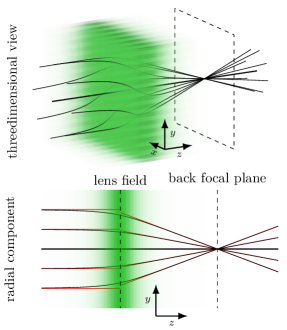
Figure 3: Paraxial optics of thin round lens: The trajectories are simultaneously rotated and bend toward the optical axis. The former may be eliminated by a transformation into a rotating frame of reference, the so called Larmor reference frame. The black lines are analytical trajectories through a Glaser bell-shaped field, the red lines those obtained from the transfer matrix of a thin round lens as described in this section.

Round magnetic lenses are the principal focusing devices in electron optical instruments with intermediate acceleration potential ($10$ kV - 1 MeV). They generate a confined magnetic field, which predominantly points along the straight optical axis and has rotational symmetry. Taking into account symmetry and neglecting radial dependency of the axial field in the vicinity of the optical axis, the magnetic field may be approximated with the help of Maxwell’s law $\nabla\cdot\boldsymbol{B=0}$ in cylindrical coordinates

$$\frac{\partial}{\partial\rho}\left(\rho B_{\rho}\right)=-\rho\frac{\partial}{\partial z}B_{z}\rightarrow B_{\rho}=-\frac{\rho}{2}\frac{\partial}{\partial z}B_{z}$$ (70)

or

$$\boldsymbol{B}=\underbrace{\begin{pmatrix}-\frac{\rho}{2}\frac{\partial}{\partial z}B_{z}\\ 0\\ B_{z}\end{pmatrix}}_{\textrm{cylindrical}}=\underbrace{\begin{pmatrix}-\frac{x}{2}\frac{\partial B_{z}}{\partial z}\\ -\frac{y}{2}\frac{\partial B_{z}}{\partial z}\\ B_{z}\end{pmatrix}}_{\textrm{cartesian}}\,.$$ (71)

We express the vector potentials in line gauge ensuring a vanishing $z$-component

$$\boldsymbol{A}=\begin{pmatrix}-\frac{zy}{2}\frac{\partial}{\partial z}\int\limits_{0}^{1}B_{z}\left(uz\right)udu-y\int\limits_{0}^{1}B_{z}(uz)udu\\ \frac{zx}{2}\frac{\partial}{\partial z}\int\limits_{0}^{1}B_{z}\left(uz\right)udu+x\int\limits_{0}^{1}B_{z}(uz)udu\\ 0\end{pmatrix}\,,$$ (72)

which renders the JVE for the longitudinal component trivial. The transverse components of the Jacobian of the Hamiltonian flow read

$$\chi_{xy}\left(t\right)=\frac{1}{m}\left(\begin{array}[]{cccc}0&\frac{1}{2}qB_{z}&1&0\\ -\frac{1}{2}qB_{z}&0&0&1\\ -\frac{1}{4}q^{2}B_{z}^{2}&0&0&\frac{1}{2}qB_{z}\\ 0&-\frac{1}{4}q^{2}B_{z}^{2}&-\frac{1}{2}qB_{z}&0\end{array}\right)\,.$$ (73)

The entries in the upper left and lower right $2\times 2$ block indicate that the round lens rotates the image by the Larmor frequency $\frac{qB_{z}}{2m}$.

In the next step we absorb the Larmor rotation into a rotating Larmor frame of reference by employing the ansatz $\boldsymbol{Y}=O\widetilde{\boldsymbol{Y}}$with the Larmor rotation matrix $O$. It follows that

$$\frac{d\widetilde{\boldsymbol{Y}}}{dt}=\left(o^{T}+O^{T}\chi_{x\left(t\right)}O\right)\widetilde{\boldsymbol{Y}}$$ (74)

with the infinitesimal rotation matrix

$$o=\frac{1}{m}\left(\begin{array}[]{cccc}0&\frac{1}{2}qB_{z}&0&0\\ -\frac{1}{2}qB_{z}&0&0&0\\ 0&0&0&\frac{1}{2}qB_{z}\\ 0&0&-\frac{1}{2}qB_{z}&0\end{array}\right)$$ (75)

and $O=\exp\left(to\right)$. Consequently, the JVE in the Larmor frame of reference has the Jacobian

$$\widetilde{\chi}\left(t\right) \coloneqq o^{T}+O^{T}\left(\frac{\partial X_{i}}{\partial x_{j}}\right)_{\boldsymbol{x}\left(t\right)}O$$ (76)

$$=\frac{1}{m}\left(\begin{array}[]{cccc}0&0&1&0\\ 0&0&0&1\\ -\frac{1}{4}q^{2}B_{z}^{2}&0&0&0\\ 0&-\frac{1}{4}q^{2}B_{z}^{2}&0&0\end{array}\right)_{\boldsymbol{x}\left(t\right)}\,,$$ (81)

which is very similar to that of the quadrupole (60) with the notable difference that a decoupled and identical focusing action occurs in both transverse directions. As the matrix of the system of first order differential equations depends on $t$ (via $z$$\left(t\right)$) in this case, it is, however, not possible to simply integrate the exponent before taking the matrix exponential to obtain the exact result.

Nevertheless, increasingly good approximations, which preserve the symplectic structure and hence phase space areas may be obtained with the help of the Magnus expansion (23). The first term of which corresponds to the integration of the exponent, i.e.,

$$\widetilde{M}_{xy}^{\left(I\right)} =\exp\begin{pmatrix}0&\frac{l}{mv}\\ -\frac{1}{4}\frac{q^{2}}{m}\int_{0}^{l/v}B_{z}^{2}dt&0\end{pmatrix}$$ (82)

$$=\left(\begin{array}[]{cc}\cos\left(\varphi\right)&\frac{2\sqrt{l}}{q\sqrt{\int_{0}^{l}B_{z}^{2}dz}}\sin\left(\varphi\right)\\ -\frac{q\sqrt{\int_{0}^{l}B_{z}^{2}dz}}{2\sqrt{l}}\sin\left(\varphi\right)&\cos\left(\varphi\right)\end{array}\right)$$ (85)

with

$$\varphi\coloneqq\frac{q}{2mv}\sqrt{l\int_{0}^{l}B_{z}^{2}dz}\,.$$ (86)

Note that we considered only one of the identical transverse directions here for clarity.

Similar to that of quadrupole, the chosen gauge implies that the kinetic and canonical momentum coincide. The focal length for the weak lens $\varphi\ll 1$ then reads $\frac{1}{f}=\frac{1}{4}\frac{q^{2}}{\left(mv\right)^{2}}\int_{0}^{l}B_{z}^{2}dz$, which corresponds exactly to famous Busch’s formula for the focusing action of a thin lens [20]. Up to second order the Magnus expansion (23) involves a commutator

$$\left[\widetilde{\chi}\left(t\right),\widetilde{\chi}\left(t_{1}\right)\right]=\frac{q^{2}\left(B_{z}^{2}\left(t\right)-B_{z}^{2}\left(t_{1}\right)\right)}{4m^{2}}\left(\begin{array}[]{cc}1&0\\ 0&-1\end{array}\right)$$ (87)

of the Jacobian $\chi\left(t\right)$ matrix of the JVE (11) and reads

$$\widetilde{M}_{xy}^{\left(II\right)} =\exp\left(\int_{0}^{l/v}dt\widetilde{\chi}_{ij}\left(t\right)+\frac{1}{2}\int_{0}^{l/v}dt\int_{0}^{t}dt_{1}\left[\widetilde{\chi}_{ij}\left(t\right),\widetilde{\chi}_{ij}\left(t_{1}\right)\right]\right)$$ (88)

$$=\exp\begin{pmatrix}\frac{q^{2}}{8m^{2}}\int_{0}^{l/v}\left(B_{z}^{2}t-\int_{0}^{t}B_{z}^{2}dt_{1}\right)dt&\frac{l}{mv}\\ -\frac{q^{2}}{4m}\int_{0}^{l/v}B_{z}^{2}dt&-\frac{q^{2}}{8m^{2}}\int_{0}^{l/v}\left(B_{z}^{2}t-\int_{0}^{t}B_{z}^{2}dt_{1}\right)dt\end{pmatrix}$$

The latter may be further simplified by partial integration if the initial and final plane considered are outside the field of the lens

$$\widetilde{M}_{xy}^{\left(II\right)} =\exp\begin{pmatrix}\frac{q^{2}}{4m^{2}}\int_{0}^{l/v}B_{z}^{2}tdt&\frac{l}{mv}\\ -\frac{q^{2}}{4m}\int_{0}^{l/v}B_{z}^{2}dt&-\frac{q^{2}}{4m^{2}}\int_{0}^{l/v}\int_{0}^{t}B_{z}^{2}dt\end{pmatrix}$$ (89)

$$=\left(\begin{array}[]{cc}\frac{q^{2}\int_{0}^{l}B_{z}^{2}zdz\,\sin\left(\varphi\right)}{4m^{2}v^{2}\varphi}+\cos\left(\varphi\right)&\frac{l\sin\left(\varphi\right)}{\gamma mv\varphi}\\ -\frac{q^{2}\int_{0}^{l}B_{z}^{2}dz\,\sin\left(\varphi\right)}{4mv\varphi}&\frac{-q^{2}\int_{0}^{l}B_{z}^{2}zdz\,\sin\left(\varphi\right)}{4m^{2}v^{2}\varphi}+\cos\left(\varphi\right)\end{array}\right)$$ (92)

with

$$\varphi\coloneqq\frac{q}{2m}\sqrt{\frac{l}{v^{2}}\int_{0}^{l}B_{z}^{2}dz-\frac{q^{2}}{4m^{2}v}\left(\int_{0}^{l}B_{z}^{2}dz\right)^{2}}\,.$$ (93)

It is readily verified that ($\tilde{M}_{xy}^{\left(II\right)}$) is again symplectic. A detailed comparison of such higher-order Magnus expansions with paraxial trajectories obtained by numerical step solvers (or exact solutions of the Glaser field) is warranted to beyond the scope of this paper and will be conducted elsewhere. Depending on the required accuracy, such explicit transfer matrix expressions may be used to derive more accurate expressions of aberrations integrals of round lenses. Similarly improved closed expression can be also derived for the inhomogeneous quadrupole (e.g., including fringing fields) or the following devices.

B.3 Wien Filter

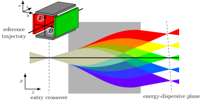
Figure 4: Paraxial optics of a Wien filter. As the longitudinal deviations are not causing any additional transverse deflections, they are not shown.

CPO devices with non-zero transverse magnetic and electrostatic fields along the optical axis are used predominantly as deflectors and spectrometers. The Wien filter is such a device that employs crossed electric and magnetic fields to separate charged particles according to their velocity (in case of charged particles of the same $q/m$ ratio) or mass (in case of ions of defined energy with different $q/m$ ratio). It has the unique property (among velocity filters) of a straight reference trajectory, i.e., the optical axis $x$ (see Fig. 4). In the following, we will again consider only the homogeneous case (i.e., the inner region of the filter), which contains only constant electric and magnetic fields

$$\boldsymbol{B}=\begin{pmatrix}0\\ B_{y}\\ 0\end{pmatrix}\,,\boldsymbol{E}=\begin{pmatrix}E_{x}=vB_{y}\\ 0\\ 0\end{pmatrix}$$ (94)

which are perpendicular and obey a fixed relationship ensuring a straight reference trajectory. The vector potential in a convenient gauge $(A_{x}=A_{y}=0)$ reads

$$\mathbf{A}(\mathbf{r})=\begin{pmatrix}0\\ 0\\ -B_{y}x\end{pmatrix}\,.$$ (95)

yielding the following Hamilton flow Jacobian (11) for the deviations in $x$- and $z$-direction ($y$ is a trivial drift)

$$\chi_{xz}=\frac{1}{m}\left(\begin{array}[]{cccc}0&-qB_{y}&1&0\\ 0&0&0&1\\ 0&0&0&0\\ 0&-q^{2}B_{y}^{2}&qB_{y}&0\end{array}\right)\,.$$ (96)

In contrast to the quadrupole, the sharp cut-off field additionally modifies the paraxial trajectory in phase space by introducing a sharp jump in the transverse momentum at the entrance and exit plane. Indeed, the latter corresponds to the gauge transformation in the initial and final plane discussed further below. As the Hamilton flow Jacobian is time-invariant, the transfer matrices for a Wien filter of length $l$ can be obtained easily by integrating the Jacobian $\boldsymbol{\chi}$ and taking the matrix exponential

$$\mathcal{M}_{xz} =\exp\left(\begin{array}[]{cccc}0&0&\frac{l}{mv}&0\\ qB_{y}\frac{l}{mv}&0&0&\frac{l}{mv}\\ -q^{2}B_{y}^{2}\frac{l}{mv}&0&0&-qB_{y}\frac{l}{mv}\\ 0&0&0&0\end{array}\right)$$ (101)

$$=\left(\begin{array}[]{cccc}\cos\varphi&0&\frac{\sin\varphi}{qB_{y}}&\frac{\cos\varphi-1}{qB_{y}}\\ \sin\varphi&1&-\frac{\cos\varphi-1}{qB_{y}}&\frac{\sin\varphi}{qB_{y}}\\ -qB_{y}\sin\varphi&0&\cos\varphi&-\sin\varphi\\ 0&0&0&1\end{array}\right)$$ (106)

with $\varphi\coloneqq qB_{y}\frac{l}{mv}$. To obtain the gauge-independent kinetic momentum transfer we can exploit that the gauge linearly depends on the spatial coordinates, which relates the canonical and kinetic transfer matrices by a similarity transformation (21), yielding

$$M_{xz} =\left(\begin{array}[]{cccc}1&0&0&0\\ 0&1&0&0\\ 0&0&1&0\\ qB_{y}&0&0&1\end{array}\right)\mathcal{M}_{xz}\left(\begin{array}[]{cccc}1&0&0&0\\ 0&1&0&0\\ 0&0&1&0\\ -qB_{y}&0&0&1\end{array}\right)$$ (115)

$$=\left(\begin{array}[]{cccc}1&0&\frac{\sin\varphi}{qB_{y}}&\frac{\cos\varphi-1}{qB_{y}}\\ 0&1&-\frac{\cos\varphi-1}{qB_{y}}&\frac{\sin\varphi}{qB_{y}}\\ 0&0&\cos\varphi&-\sin\varphi\\ 0&0&\sin\varphi&\cos\varphi\end{array}\right)\,,$$ (120)

and

$$M_{y}=\begin{pmatrix}1&\frac{l}{p_{0}}\\ 0&1\end{pmatrix}\,,$$ (121)

This result coincides with that obtained from the Newtonian equations of motion. Note that the lower left sector of $M_{xz}$ is empty, which means that the Wien filter acts similar to a telescope. Notwithstanding, a point on the optical axis is imaged into a point, with the position of the focal point depending on the initial longitudinal momentum (see Fig. 4), which is the determining property in energy filter and spectrometer applications. We finally note that initial momentum deviations also entail longitudinal deviations in the final plane. These may be, however, neglected in the paraxial limit because the pertaining additional propagation along the straight optical axis do not induce any additional transversal deviations (see below for another example, where this is not the case).

The first order aberrations are determined completely by time lag aberrations (35) because

$$\left(\frac{\partial X_{i}}{\partial x_{j}\partial x_{k}}\right)_{x\left(t\right)}=0\,.$$ (122)

Taking into account gauge, we have to evaluate

$$M_{il_{1}l_{2}}^{\left(2t\right)}=G_{ii_{1}}\left(t\right)\mathcal{M}_{i_{1}j_{1}j_{2}}^{\left(2t\right)}G_{j_{1}l_{1}}^{-1}\left(0\right)G_{j_{1}l_{1}}^{-1}\left(0\right)$$ (123)

yielding

$$C_{144} =-\frac{\cos\varphi\left(\cos\varphi-1\right)}{qB_{y}p_{0}}$$

$$C_{146} =-\frac{\sin\varphi\left(2\cos\varphi-1\right)}{qB_{y}p_{0}}$$

$$C_{166} =\frac{\sin^{2}\varphi}{qB_{y}p_{0}}$$

$$C_{254} =\frac{\cos\varphi-1}{qB_{y}p_{0}}$$

$$C_{256} =-\frac{\sin\varphi}{qB_{y}p_{0}}$$

These are the aberrations of the Wien filter with sharp cut-off fields. For a comprehensive analytic treatment including higher orders and fringing fields see Ref. [21].

B.4 Sector Magnet

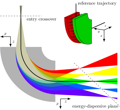
Figure 5: Paraxial optics of a sector magnet. Note that the coordinate system is turned alongside the reference trajectory after the exit plane.

Sector magnets refer to opposing magnetic pole piece geometries being limited by entrance and exit planes such to create a sector of a circle (see Fig. 5). They find application in spectrometers, energy filters, particle separators as well as beam guiding systems. Considering again the case of homogeneous fields only (i.e., parallel pole pieces with sharp cut-off), we can directly copy the transfer matrix of the Wien filter in the $x-z$ plane

$$M=\left(\begin{array}[]{cccc}1&0&\frac{\sin\varphi}{qB_{z}}&\frac{\cos\varphi-1}{qB_{z}}\\ 0&1&-\frac{\cos\varphi-1}{qB_{z}}&\frac{\sin\varphi}{qB_{z}}\\ 0&0&\cos\varphi&-\sin\varphi\\ 0&0&\sin\varphi&\cos\varphi\end{array}\right)\,.$$ (125)

We again note the missing dependency of the final kinetic momentum on the initial position, which, contrary to the Wien filter, however, does not imply a missing focusing action, i.e., an induced convergence of parallel trajectories, in the sector magnet. The latter is induced by considering that longitudinal deviations (see Fig. 5) effectively introduce an additional deflection due to additional propagation lengthsdepending linearly on the initial beam position. To illustrate that point we first compute the time of flight $\delta t$ required for the particle to cover that longitudinal shift by projecting the spacial part of the deviation vector on the tangent of the optical axis

$$-\sin\varphi X_{1}\left(t\right)+\cos\varphi X_{3}\left(t\right)\approx\omega R\delta t\,,$$ (126)

and hence

$$\delta t \approx\frac{-\sin\varphi X_{1}\left(t\right)+\cos\varphi X_{3}\left(t\right)}{\omega R}\,.$$ (127)

Adding the ensuing additional propagation along the optical axis to the particle we obtain the first order additional deviation of the beam

$$\boldsymbol{X}^{\prime}\left(t\right) =\omega\left(\begin{array}[]{cccc}0&-\delta t&0&0\\ \delta t&0&0&0\\ 0&0&0&-\delta t\\ 0&0&\delta t&0\end{array}\right)\boldsymbol{x}\left(t\right)$$ (132)

$$=R\omega\left(\begin{array}[]{cccc}0&-\delta t&0&0\\ \delta t&0&0&0\\ 0&0&0&-\delta t\\ 0&0&\delta t&0\end{array}\right)\begin{pmatrix}\cos\varphi\\ \sin\varphi\\ -\gamma m\omega\sin\varphi\\ \gamma m\omega\cos\varphi\end{pmatrix}$$ (137)

$$=R\omega\begin{pmatrix}-\sin\varphi\\ \cos\varphi\\ -qB_{z}\cos\varphi\\ -qB_{z}\sin\varphi\end{pmatrix}\delta t$$

$$=\left(\begin{array}[]{cccc}\sin^{2}\varphi&-\sin\varphi\cos\varphi&0&0\\ -\cos\varphi\sin\varphi&\cos^{2}\varphi&0&0\\ qB_{z}\cos\varphi\sin\varphi&-qB_{z}\cos^{2}\varphi&0&0\\ qB_{z}\sin^{2}\varphi&-qB_{z}\cos\varphi\sin\varphi&0&0\end{array}\right)\boldsymbol{X}\left(t\right)$$ (142)

$$=M^{\prime}\boldsymbol{X}\left(0\right)$$

with

$$M^{\prime}=\left(\begin{array}[]{cccc}\sin^{2}\varphi&-\sin\varphi\cos\varphi&0&0\\ -\cos\varphi\sin\varphi&\cos^{2}\varphi&0&0\\ qB_{z}\cos\varphi\sin\varphi&-qB_{z}\cos^{2}\varphi&0&0\\ qB_{z}\sin^{2}\varphi&-qB_{z}\cos\varphi\sin\varphi&0&0\end{array}\right)M\,.$$ (143)

The additional deviation $\boldsymbol{X}^{\prime}\left(t\right)$ needs to be added to the final $\boldsymbol{X}\left(t\right)$ to obtain the correct deviation in the image plane, which can be alternatively written as $\boldsymbol{X}^{\prime}\left(t\right)+\boldsymbol{X}\left(t\right)=\mathscr{M}\boldsymbol{X}\left(0\right)$ defining a modified transfer matrix

$$\mathscr{\mathscr{M}} \coloneqq O\left(M+M^{\prime}\right)$$ (144)

$$=\left(\begin{array}[]{cccc}\cos\varphi&\sin\varphi&0&0\\ -\sin\varphi&\cos\varphi&0&0\\ 0&0&\cos\varphi&\sin\varphi\\ 0&0&-\sin\varphi&\cos\varphi\end{array}\right)\left(M+M^{\prime}\right)$$ (149)

$$=\left(\begin{array}[]{cccc}\cos\varphi&\sin\varphi&\frac{\sin\varphi}{qB_{z}}&\frac{1-\cos\varphi}{qB_{z}}\\ 0&0&0&0\\ -qB_{z}\sin\varphi&qB_{z}\cos\varphi&\cos\varphi&\sin\varphi\\ 0&0&0&1\end{array}\right)$$ (154)

Here we have incorporated an additional rotation $O$ transforming the vector in laboratory frame into a frame rotated with the optical axis. The obtained $\mathscr{\mathscr{M}}$ is equivalent to the classical result for the sector magnet [22, 23, 24] and exhibits the familiar focusing effect in radial direction (see lower left sector of $\mathscr{\mathscr{M}}$) including Barber’s rule [25].