EfficientNetV2: Smaller Models and Faster Training
Abstract
This paper introduces EfficientNetV2, a new family of convolutional networks that have faster training speed and better parameter efficiency than previous models. To develop these models, we use a combination of training-aware neural architecture search and scaling, to jointly optimize training speed and parameter efficiency. The models were searched from the search space enriched with new ops such as Fused-MBConv. Our experiments show that EfficientNetV2 models train much faster than state-of-the-art models while being up to 6.8x smaller.
Our training can be further sped up by progressively increasing the image size during training, but it often causes a drop in accuracy. To compensate for this accuracy drop, we propose an improved method of progressive learning, which adaptively adjusts regularization (e.g. data augmentation) along with image size.
With progressive learning, our EfficientNetV2 significantly outperforms previous models on ImageNet and CIFAR/Cars/Flowers datasets. By pretraining on the same ImageNet21k, our EfficientNetV2 achieves 87.3% top-1 accuracy on ImageNet ILSVRC2012, outperforming the recent ViT by 2.0% accuracy while training 5x-11x faster using the same computing resources. Code is available at https://github.com/google/automl/tree/master/efficientnetv2.
1 Introduction
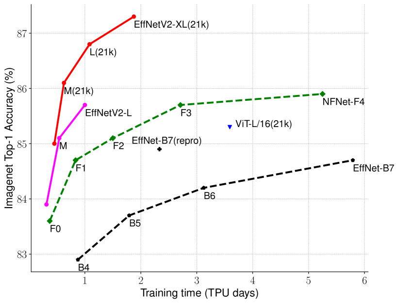
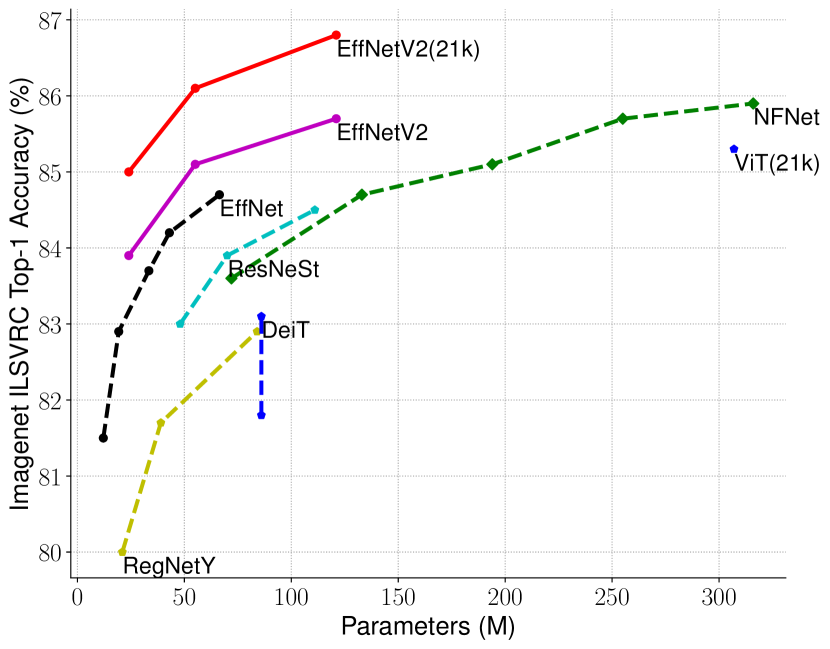
(a) Training efficiency. EfficientNet ResNet-RS DeiT/ViT EfficientNetV2 (2019) (2021) (2021) (ours) Top-1 Acc. 84.3% 84.0% 83.1% 83.9% Parameters 43M 164M 86M 24M (b) Parameter efficiency.
Training efficiency is important to deep learning as model size and training data size are increasingly larger. For example, GPT-3 (Brown et al., 2020), with much a larger model and more training data, demonstrates the remarkable capability in few shot learning, but it requires weeks of training with thousands of GPUs, making it difficult to retrain or improve.
Training efficiency has gained significant interests recently. For instance, NFNets (Brock et al., 2021) aim to improve training efficiency by removing the expensive batch normalization; Several recent works (Srinivas et al., 2021) focus on improving training speed by adding attention layers into convolutional networks (ConvNets); Vision Transformers (Dosovitskiy et al., 2021) improves training efficiency on large-scale datasets by using Transformer blocks. However, these methods often come with expensive overhead on large parameter size, as shown in Figure 1(b).
In this paper, we use an combination of training-aware neural architecture search (NAS) and scaling to improve both training speed and parameter efficiency. Given the parameter efficiency of EfficientNets (Tan & Le, 2019a), we start by systematically studying the training bottlenecks in EfficientNets. Our study shows in EfficientNets: (1) training with very large image sizes is slow; (2) depthwise convolutions are slow in early layers. (3) equally scaling up every stage is sub-optimal. Based on these observations, we design a search space enriched with additional ops such as Fused-MBConv, and apply training-aware NAS and scaling to jointly optimize model accuracy, training speed, and parameter size. Our found networks, named EfficientNetV2, train up to 4x faster than prior models (Figure 3), while being up to 6.8x smaller in parameter size.
Our training can be further sped up by progressively increasing image size during training. Many previous works, such as progressive resizing (Howard, 2018), FixRes (Touvron et al., 2019), and Mix&Match (Hoffer et al., 2019), have used smaller image sizes in training; however, they usually keep the same regularization for all image sizes, causing a drop in accuracy. We argue that keeping the same regularization for different image sizes is not ideal: for the same network, small image size leads to small network capacity and thus requires weak regularization; vice versa, large image size requires stronger regularization to combat overfitting (see Section 4.1). Based on this insight, we propose an improved method of progressive learning: in the early training epochs, we train the network with small image size and weak regularization (e.g., dropout and data augmentation), then we gradually increase image size and add stronger regularization. Built upon progressive resizing (Howard, 2018), but by dynamically adjusting regularization, our approach can speed up the training without causing accuracy drop.
With the improved progressive learning, our EfficientNetV2 achieves strong results on ImageNet, CIFAR-10, CIFAR-100, Cars, and Flowers dataset. On ImageNet, we achieve 85.7% top-1 accuracy while training 3x - 9x faster and being up to 6.8x smaller than previous models (Figure 1). Our EfficientNetV2 and progressive learning also make it easier to train models on larger datasets. For example, ImageNet21k (Russakovsky et al., 2015) is about 10x larger than ImageNet ILSVRC2012, but our EfficientNetV2 can finish the training within two days using moderate computing resources of 32 TPUv3 cores. By pretraining on the public ImageNet21k, our EfficientNetV2 achieves 87.3% top-1 accuracy on ImageNet ILSVRC2012, outperforming the recent ViT-L/16 by 2.0% accuracy while training 5x-11x faster (Figure 1).
Our contributions are threefold:
-
•
We introduce EfficientNetV2, a new family of smaller and faster models. Found by our training-aware NAS and scaling, EfficientNetV2 outperform previous models in both training speed and parameter efficiency.
-
•
We propose an improved method of progressive learning, which adaptively adjusts regularization along with image size. We show that it speeds up training, and simultaneously improves accuracy.
-
•
We demonstrate up to 11x faster training speed and up to 6.8x better parameter efficiency on ImageNet, CIFAR, Cars, and Flowers dataset, than prior art.
2 Related work
Training and parameter efficiency:
Many works, such as DenseNet (Huang et al., 2017) and EfficientNet (Tan & Le, 2019a), focus on parameter efficiency, aiming to achieve better accuracy with less parameters. Some more recent works aim to improve training or inference speed instead of parameter efficiency. For example, RegNet (Radosavovic et al., 2020), ResNeSt (Zhang et al., 2020), TResNet (Ridnik et al., 2020), and EfficientNet-X (Li et al., 2021) focus on GPU and/or TPU inference speed; NFNets (Brock et al., 2021) and BoTNets (Srinivas et al., 2021) focus on improving training speed. However, their training or inference speed often comes with the cost of more parameters. This paper aims to significantly improve both training speed and parameter efficiency than prior art.
Progressive training:
Previous works have proposed different kinds of progressive training, which dynamically change the training settings or networks, for GANs (Karras et al., 2018), transfer learning (Karras et al., 2018), adversarial learning (Yu et al., 2019), and language models (Press et al., 2021). Progressive resizing (Howard, 2018) is mostly related to our approach, which aims to improve training speed. However, it usually comes with the cost of accuracy drop. Another closely related work is Mix&Match (Hoffer et al., 2019), which randomly sample different image size for each batch. Both progressive resizing and Mix&Match use the same regularization for all image sizes, causing a drop in accuracy. In this paper, our main difference is to adaptively adjust regularization as well so that we can improve both training speed and accuracy. Our approach is also partially inspired by curriculum learning (Bengio et al., 2009), which schedules training examples from easy to hard. Our approach also gradually increases learning difficulty by adding more regularization, but we don’t selectively pick training examples.
Neural architecture search (NAS):
By automating the network design process, NAS has been used to optimize the network architecture for image classification (Zoph et al., 2018), object detection (Chen et al., 2019; Tan et al., 2020), segmentation (Liu et al., 2019), hyperparameters (Dong et al., 2020), and other applications (Elsken et al., 2019). Previous NAS works mostly focus on improving FLOPs efficiency (Tan & Le, 2019b, a) or inference efficiency (Tan et al., 2019; Cai et al., 2019; Wu et al., 2019; Li et al., 2021). Unlike prior works, this paper uses NAS to optimize training and parameter efficiency.
3 EfficientNetV2 Architecture Design
In this section, we study the training bottlenecks of EfficientNet (Tan & Le, 2019a), and introduce our training-aware NAS and scaling, as well as EfficientNetV2 models.
3.1 Review of EfficientNet
EfficientNet (Tan & Le, 2019a) is a family of models that are optimized for FLOPs and parameter efficiency. It leverages NAS to search for the baseline EfficientNet-B0 that has better trade-off on accuracy and FLOPs. The baseline model is then scaled up with a compound scaling strategy to obtain a family of models B1-B7. While recent works have claimed large gains on training or inference speed, they are often worse than EfficientNet in terms of parameters and FLOPs efficiency (Table 1). In this paper, we aim to improve the training speed while maintaining the parameter efficiency.
3.2 Understanding Training Efficiency
We study the training bottlenecks of EfficientNet (Tan & Le, 2019a), henceforth is also called EfficientNetV1, and a few simple techniques to improve training speed.
Training with very large image sizes is slow:
As pointed out by previous works (Radosavovic et al., 2020), EfficientNet’s large image size results in significant memory usage. Since the total memory on GPU/TPU is fixed, we have to train these models with smaller batch size, which drastically slows down the training. A simple improvement is to apply FixRes (Touvron et al., 2019), by using a smaller image size for training than for inference. As shown in Table 2, smaller image size leads to less computations and enables large batch size, and thus improves training speed by up to 2.2x. Notably, as pointed out in (Touvron et al., 2020; Brock et al., 2021), using smaller image size for training also leads to slightly better accuracy. But unlike (Touvron et al., 2019), we do not finetune any layers after training.
| TPUv3 imgs/sec/core | V100 imgs/sec/gpu | ||||
|---|---|---|---|---|---|
| Top-1 Acc. | batch=32 | batch=128 | batch=12 | batch=24 | |
| train size=512 | 84.3% | 42 | OOM | 29 | OOM |
| train size=380 | 84.6% | 76 | 93 | 37 | 52 |
In Section 4, we will explore a more advanced training approach, by progressively adjusting image size and regularization during training.
Depthwise convolutions are slow in early layers but effective in later stages:
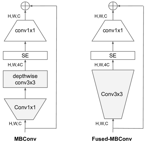
Another training bottleneck of EfficientNet comes from the extensive depthwise convolutions (Sifre, 2014). Depthwise convolutions have fewer parameters and FLOPs than regular convolutions, but they often cannot fully utilize modern accelerators. Recently, Fused-MBConv is proposed in (Gupta & Tan, 2019) and later used in (Gupta & Akin, 2020; Xiong et al., 2020; Li et al., 2021) to better utilize mobile or server accelerators. It replaces the depthwise conv3x3 and expansion conv1x1 in MBConv (Sandler et al., 2018; Tan & Le, 2019a) with a single regular conv3x3, as shown in Figure 2. To systematically compares these two building blocks, we gradually replace the original MBConv in EfficientNet-B4 with Fused-MBConv (Table 3). When applied in early stage 1-3, Fused-MBConv can improve training speed with a small overhead on parameters and FLOPs, but if we replace all blocks with Fused-MBConv (stage 1-7), then it significantly increases parameters and FLOPs while also slowing down the training. Finding the right combination of these two building blocks, MBConv and Fused-MBConv, is non-trivial, which motivates us to leverage neural architecture search to automatically search for the best combination.
| Params | FLOPs | Top-1 | TPU | V100 | |
|---|---|---|---|---|---|
| (M) | (B) | Acc. | imgs/sec/core | imgs/sec/gpu | |
| No fused | 19.3 | 4.5 | 82.8% | 262 | 155 |
| Fused stage1-3 | 20.0 | 7.5 | 83.1% | 362 | 216 |
| Fused stage1-5 | 43.4 | 21.3 | 83.1% | 327 | 223 |
| Fused stage1-7 | 132.0 | 34.4 | 81.7% | 254 | 206 |
Equally scaling up every stage is sub-optimal:
EfficientNet equally scales up all stages using a simple compound scaling rule. For example, when depth coefficient is 2, then all stages in the networks would double the number of layers. However, these stages are not equally contributed to the training speed and parameter efficiency. In this paper, we will use a non-uniform scaling strategy to gradually add more layers to later stages. In addition, EfficientNets aggressively scale up image size, leading to large memory consumption and slow training. To address this issue, we slightly modify the scaling rule and restrict the maximum image size to a smaller value.
3.3 Training-Aware NAS and Scaling
To this end, we have learned multiple design choices for improving training speed. To search for the best combinations of those choices, we now propose a training-aware NAS.
NAS Search:
Our training-aware NAS framework is largely based on previous NAS works (Tan et al., 2019; Tan & Le, 2019a), but aims to jointly optimize accuracy, parameter efficiency, and training efficiency on modern accelerators. Specifically, we use EfficientNet as our backbone. Our search space is a stage-based factorized space similar to (Tan et al., 2019), which consists of the design choices for convolutional operation types {MBConv, Fused-MBConv}, number of layers, kernel size {3x3, 5x5}, expansion ratio {1, 4, 6}. On the other hand, we reduce the search space size by (1) removing unnecessary search options such as pooling skip ops, since they are never used in the original EfficientNets; (2) reusing the same channel sizes from the backbone as they are already searched in (Tan & Le, 2019a). Since the search space is smaller, we can apply reinforcement learning (Tan et al., 2019) or simply random search on much larger networks that have comparable size as EfficientNet-B4. Specifically, we sample up to 1000 models and train each model about 10 epochs with reduced image size for training. Our search reward combines the model accuracy , the normalized training step time , and the parameter size , using a simple weighted product , where = -0.07 and = -0.05 are empirically determined to balance the trade-offs similar to (Tan et al., 2019).
EfficientNetV2 Architecture:
Table 4 shows the architecture for our searched model EfficientNetV2-S. Compared to the EfficientNet backbone, our searched EfficientNetV2 has several major distinctions: (1) The first difference is EfficientNetV2 extensively uses both MBConv (Sandler et al., 2018; Tan & Le, 2019a) and the newly added fused-MBConv (Gupta & Tan, 2019) in the early layers. (2) Secondly, EfficientNetV2 prefers smaller expansion ratio for MBConv since smaller expansion ratios tend to have less memory access overhead. (3) Thirdly, EfficientNetV2 prefers smaller 3x3 kernel sizes, but it adds more layers to compensate the reduced receptive field resulted from the smaller kernel size. (4) Lastly, EfficientNetV2 completely removes the last stride-1 stage in the original EfficientNet, perhaps due to its large parameter size and memory access overhead.
| Stage | Operator | Stride | #Channels | #Layers |
|---|---|---|---|---|
| 0 | Conv3x3 | 2 | 24 | 1 |
| 1 | Fused-MBConv1, k3x3 | 1 | 24 | 2 |
| 2 | Fused-MBConv4, k3x3 | 2 | 48 | 4 |
| 3 | Fused-MBConv4, k3x3 | 2 | 64 | 4 |
| 4 | MBConv4, k3x3, SE0.25 | 2 | 128 | 6 |
| 5 | MBConv6, k3x3, SE0.25 | 1 | 160 | 9 |
| 6 | MBConv6, k3x3, SE0.25 | 2 | 256 | 15 |
| 7 | Conv1x1 & Pooling & FC | - | 1280 | 1 |
EfficientNetV2 Scaling:
We scale up EfficientNetV2-S to obtain EfficientNetV2-M/L using similar compound scaling as (Tan & Le, 2019a), with a few additional optimizations: (1) we restrict the maximum inference image size to 480, as very large images often lead to expensive memory and training speed overhead; (2) as a heuristic, we also gradually add more layers to later stages (e.g., stage 5 and 6 in Table 4) in order to increase the network capacity without adding much runtime overhead.
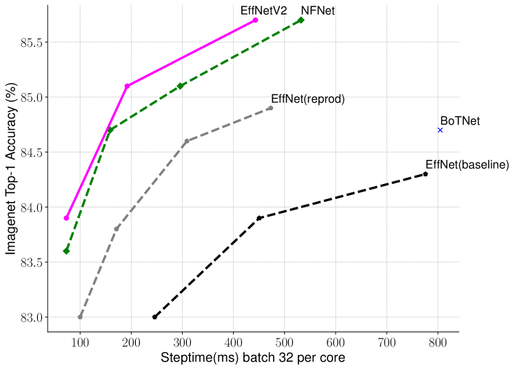
Training Speed Comparison:
Figure 3 compares the training step time for our new EfficientNetV2, where all models are trained with fixed image size without progressive learning. For EfficientNet (Tan & Le, 2019a), we show two curves: one is trained with the original inference size, and the other is trained with about 30% smaller image size, same as EfficientNetV2 and NFNet (Touvron et al., 2019; Brock et al., 2021). All models are trained with 350 epochs, except NFNets are trained with 360 epochs, so all models have a similar number of training steps. Interestingly, we observe that when trained properly, EfficientNets still achieve pretty strong performance trade-off. More importantly, with our training-aware NAS and scaling, our proposed EfficientNetV2 model train much faster than the other recent models. These results also align with our inference results as shown in Table 7 and Figure 5.
4 Progressive Learning
4.1 Motivation
As discussed in Section 3, image size plays an important role in training efficiency. In addition to FixRes (Touvron et al., 2019), many other works dynamically change image sizes during training (Howard, 2018; Hoffer et al., 2019), but they often cause a drop in accuracy.
We hypothesize the accuracy drop comes from the unbalanced regularization: when training with different image sizes, we should also adjust the regularization strength accordingly (instead of using a fixed regularization as in previous works). In fact, it is common that large models require stronger regularization to combat overfitting: for example, EfficientNet-B7 uses larger dropout and stronger data augmentation than the B0. In this paper, we argue that even for the same network, smaller image size leads to smaller network capacity and thus needs weaker regularization; vice versa, larger image size leads to more computations with larger capacity, and thus more vulnerable to overfitting.
To validate our hypothesis, we train a model, sampled from our search space, with different image sizes and data augmentations (Table 5). When image size is small, it has the best accuracy with weak augmentation; but for larger images, it performs better with stronger augmentation. This insight motivates us to adaptively adjust regularization along with image size during training, leading to our improved method of progressive learning.
| Size=128 | Size=192 | Size=300 | |
|---|---|---|---|
| RandAug magnitude=5 | 78.3 0.16 | 81.2 0.06 | 82.5 0.05 |
| RandAug magnitude=10 | 78.0 0.08 | 81.6 0.08 | 82.7 0.08 |
| RandAug magnitude=15 | 77.7 0.15 | 81.5 0.05 | 83.2 0.09 |
4.2 Progressive Learning with adaptive Regularization
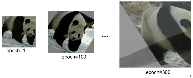
Figure 4 illustrates the training process of our improved progressive learning: in the early training epochs, we train the network with smaller images and weak regularization, such that the network can learn simple representations easily and fast. Then, we gradually increase image size but also making learning more difficult by adding stronger regularization. Our approach is built upon (Howard, 2018) that progressively changes image size, but here we adaptively adjust regularization as well.
Formally, suppose the whole training has total steps, the target image size is , with a list of regularization magnitude , where represents a type of regularization such as dropout rate or mixup rate value. We divide the training into stages: for each stage , the model is trained with image size and regularization magnitude . The last stage would use the targeted image size and regularization . For simplicity, we heuristically pick the initial image size and regularization , and then use a linear interpolation to determine the value for each stage. Algorithm 1 summarizes the procedure. At the beginning of each stage, the network will inherit all weights from the previous stage. Unlike transformers, whose weights (e.g., position embedding) may depend on input length, ConvNet weights are independent to image sizes and thus can be inherited easily.
Our improved progressive learning is generally compatible to existing regularization. For simplicity, this paper mainly studies the following three types of regularization:
-
•
Dropout (Srivastava et al., 2014): a network-level regularization, which reduces co-adaptation by randomly dropping channels. We will adjust the dropout rate .
-
•
RandAugment (Cubuk et al., 2020): a per-image data augmentation, with adjustable magnitude .
-
•
Mixup (Zhang et al., 2018): a cross-image data augmentation. Given two images with labels (, ) and (, ), it combines them with mixup ratio : and . We would adjust mixup ratio during training.
5 Main Results
This section presents our experimental setups, the main results on ImageNet, and the transfer learning results on CIFAR-10, CIFAR-100, Cars, and Flowers.
5.1 ImageNet ILSVRC2012
Setup:
ImageNet ILSVRC2012 (Russakovsky et al., 2015) contains about 1.28M training images and 50,000 validation images with 1000 classes. During architecture search or hyperparameter tuning, we reserve 25,000 images (about 2%) from the training set as minival for accuracy evaluation. We also use minival to perform early stopping. Our ImageNet training settings largely follow EfficientNets (Tan & Le, 2019a): RMSProp optimizer with decay 0.9 and momentum 0.9; batch norm momentum 0.99; weight decay 1e-5. Each model is trained for 350 epochs with total batch size 4096. Learning rate is first warmed up from 0 to 0.256, and then decayed by 0.97 every 2.4 epochs. We use exponential moving average with 0.9999 decay rate, RandAugment (Cubuk et al., 2020), Mixup (Zhang et al., 2018), Dropout (Srivastava et al., 2014), and stochastic depth (Huang et al., 2016) with 0.8 survival probability.
| S | M | L | ||||
| min | max | min | max | min | max | |
| Image Size | 128 | 300 | 128 | 380 | 128 | 380 |
| RandAugment | 5 | 15 | 5 | 20 | 5 | 25 |
| Mixup alpha | 0 | 0 | 0 | 0.2 | 0 | 0.4 |
| Dropout rate | 0.1 | 0.3 | 0.1 | 0.4 | 0.1 | 0.5 |
| Model | Top-1 Acc. | Params | FLOPs | Infer-time(ms) | Train-time (hours) | |
|---|---|---|---|---|---|---|
| ConvNets & Hybrid | EfficientNet-B3 (Tan & Le, 2019a) | 81.5% | 12M | 1.9B | 19 | 10 |
| EfficientNet-B4 (Tan & Le, 2019a) | 82.9% | 19M | 4.2B | 30 | 21 | |
| EfficientNet-B5 (Tan & Le, 2019a) | 83.7% | 30M | 10B | 60 | 43 | |
| EfficientNet-B6 (Tan & Le, 2019a) | 84.3% | 43M | 19B | 97 | 75 | |
| EfficientNet-B7 (Tan & Le, 2019a) | 84.7% | 66M | 38B | 170 | 139 | |
| RegNetY-8GF (Radosavovic et al., 2020) | 81.7% | 39M | 8B | 21 | - | |
| RegNetY-16GF (Radosavovic et al., 2020) | 82.9% | 84M | 16B | 32 | - | |
| ResNeSt-101 (Zhang et al., 2020) | 83.0% | 48M | 13B | 31 | - | |
| ResNeSt-200 (Zhang et al., 2020) | 83.9% | 70M | 36B | 76 | - | |
| ResNeSt-269 (Zhang et al., 2020) | 84.5% | 111M | 78B | 160 | - | |
| TResNet-L (Ridnik et al., 2020) | 83.8% | 56M | - | 45 | - | |
| TResNet-XL (Ridnik et al., 2020) | 84.3% | 78M | - | 66 | - | |
| EfficientNet-X (Li et al., 2021) | 84.7% | 73M | 91B | - | - | |
| NFNet-F0 (Brock et al., 2021) | 83.6% | 72M | 12B | 30 | 8.9 | |
| NFNet-F1 (Brock et al., 2021) | 84.7% | 133M | 36B | 70 | 20 | |
| NFNet-F2 (Brock et al., 2021) | 85.1% | 194M | 63B | 124 | 36 | |
| NFNet-F3 (Brock et al., 2021) | 85.7% | 255M | 115B | 203 | 65 | |
| NFNet-F4 (Brock et al., 2021) | 85.9% | 316M | 215B | 309 | 126 | |
| LambdaResNet-420-hybrid (Bello, 2021) | 84.9% | 125M | - | - | 67 | |
| BotNet-T7-hybrid (Srinivas et al., 2021) | 84.7% | 75M | 46B | - | 95 | |
| BiT-M-R152x2 (21k) (Kolesnikov et al., 2020) | 85.2% | 236M | 135B | 500 | - | |
| Vision Transformers | ViT-B/32 (Dosovitskiy et al., 2021) | 73.4% | 88M | 13B | 13 | - |
| ViT-B/16 (Dosovitskiy et al., 2021) | 74.9% | 87M | 56B | 68 | - | |
| DeiT-B (ViT+reg) (Touvron et al., 2021) | 81.8% | 86M | 18B | 19 | - | |
| DeiT-B-384 (ViT+reg) (Touvron et al., 2021) | 83.1% | 86M | 56B | 68 | - | |
| T2T-ViT-19 (Yuan et al., 2021) | 81.4% | 39M | 8.4B | - | - | |
| T2T-ViT-24 (Yuan et al., 2021) | 82.2% | 64M | 13B | - | - | |
| ViT-B/16 (21k) (Dosovitskiy et al., 2021) | 84.6% | 87M | 56B | 68 | - | |
| ViT-L/16 (21k) (Dosovitskiy et al., 2021) | 85.3% | 304M | 192B | 195 | 172 | |
| ConvNets (ours) | EfficientNetV2-S | 83.9% | 22M | 8.8B | 24 | 7.1 |
| EfficientNetV2-M | 85.1% | 54M | 24B | 57 | 13 | |
| EfficientNetV2-L | 85.7% | 120M | 53B | 98 | 24 | |
| EfficientNetV2-S (21k) | 84.9% | 22M | 8.8B | 24 | 9.0 | |
| EfficientNetV2-M (21k) | 86.2% | 54M | 24B | 57 | 15 | |
| EfficientNetV2-L (21k) | 86.8% | 120M | 53B | 98 | 26 | |
| EfficientNetV2-XL (21k) | 87.3% | 208M | 94B | - | 45 | |
| We do not include models pretrained on non-public Instagram/JFT images, or models with extra distillation or ensemble. | ||||||
For progressive learning, we divide the training process into four stages with about 87 epochs per stage: the early stage uses a small image size with weak regularization, while the later stages use larger image sizes with stronger regularization, as described in Algorithm 1. Table 6 shows the minimum (for the first stage) and maximum (for the last stage) values of image size and regularization. For simplicity, all models use the same minimum values of size and regularization, but they adopt different maximum values, as larger models generally require more regularization to combat overfitting. Following (Touvron et al., 2020), our maximum image size for training is about 20% smaller than inference, but we don’t finetune any layers after training.
Results:
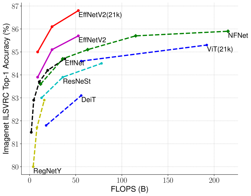
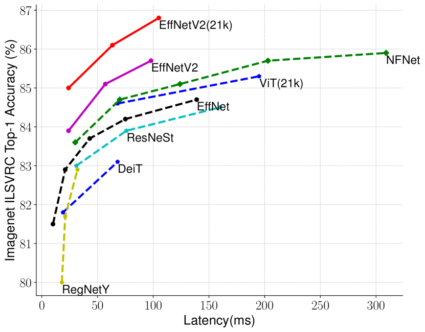
As shown in Table 7, our EfficientNetV2 models are significantly faster and achieves better accuracy and parameter efficiency than previous ConvNets and Transformers on ImageNet. In particular, our EfficientNetV2-M achieves comparable accuracy to EfficientNet-B7 while training 11x faster using the same computing resources. Our EfficientNetV2 models also significantly outperform all recent RegNet and ResNeSt, in both accuracy and inference speed. Figure 1 further visualizes the comparison on training speed and parameter efficiency. Notably, this speedup is a combination of progressive training and better networks, and we will study the individual impact for each of them in our ablation studies.
Recently, Vision Transformers have demonstrated impressive results on ImageNet accuracy and training speed. However, here we show that properly designed ConvNets with improved training method can still largely outperform vision transformers in both accuracy and training efficiency. In particular, our EfficientNetV2-L achieves 85.7% top-1 accuracy, surpassing ViT-L/16(21k), a much larger transformer model pretrained on a larger ImageNet21k dataset. Here, ViTs are not well tuned on ImageNet ILSVRC2012; DeiTs use the same architectures as ViTs, but achieve better results by adding more regularization.
Although our EfficientNetV2 models are optimized for training, they also perform well for inference, because training speed often correlates with inference speed. Figure 5 visualizes the model size, FLOPs, and inference latency based on Table 7. Since latency often depends on hardware and software, here we use the same PyTorch Image Models codebase (Wightman, 2021) and run all models on the same machine using the batch size 16. In general, our models have slightly better parameters/FLOPs efficiency than EfficientNets, but our inference latency is up to 3x faster than EfficientNets. Compared to the recent ResNeSt that are specially optimized for GPUs, our EfficientNetV2-M achieves 0.6% better accuracy with 2.8x faster inference speed.
5.2 ImageNet21k
Setup:
ImageNet21k (Russakovsky et al., 2015) contains about 13M training images with 21,841 classes. The original ImageNet21k doesn’t have train/eval split, so we reserve randomly picked 100,000 images as validation set and use the remaining as training set. We largely reuse the same training settings as ImageNet ILSVRC2012 with a few changes: (1) we change the training epochs to 60 or 30 to reduce training time, and use cosine learning rate decay that can adapt to different steps without extra tuning; (2) since each image has multiple labels, we normalize the labels to have sum of 1 before computing softmax loss. After pretrained on ImageNet21k, each model is finetuned on ILSVRC2012 for 15 epochs using cosine learning rate decay.
| Model | Params | ImageNet Acc. | CIFAR-10 | CIFAR-100 | Flowers | Cars | |
| ConvNets | GPipe (Huang et al., 2019) | 556M | 84.4 | 99.0 | 91.3 | 98.8 | 94.7 |
| EfficientNet-B7 (Tan & Le, 2019a) | 66M | 84.7 | 98.9 | 91.7 | 98.8 | 94.7 | |
| Vision Transformers | ViT-B/32 (Dosovitskiy et al., 2021) | 88M | 73.4 | 97.8 | 86.3 | 85.4 | - |
| ViT-B/16 (Dosovitskiy et al., 2021) | 87M | 74.9 | 98.1 | 87.1 | 89.5 | - | |
| ViT-L/32 (Dosovitskiy et al., 2021) | 306M | 71.2 | 97.9 | 87.1 | 86.4 | - | |
| ViT-L/16 (Dosovitskiy et al., 2021) | 306M | 76.5 | 97.9 | 86.4 | 89.7 | - | |
| DeiT-B (ViT+regularization) (Touvron et al., 2021) | 86M | 81.8 | 99.1 | 90.8 | 98.4 | 92.1 | |
| DeiT-B-384 (ViT+regularization) (Touvron et al., 2021) | 86M | 83.1 | 99.1 | 90.8 | 98.5 | 93.3 | |
| ConvNets (ours) | EfficientNetV2-S | 24M | 83.2 | 98.70.04 | 91.50.11 | 97.90.13 | 93.80.11 |
| EfficientNetV2-M | 55M | 85.1 | 99.00.08 | 92.20.08 | 98.50.08 | 94.60.10 | |
| EfficientNetV2-L | 121M | 85.7 | 99.10.03 | 92.30.13 | 98.80.05 | 95.10.10 |
Results:
Table 7 shows the performance comparison, where models tagged with 21k are pretrained on ImageNet21k and finetuned on ImageNet ILSVRC2012. Compared to the recent ViT-L/16(21k), our EfficientNetV2-L(21k) improves the top-1 accuracy by 1.5% (85.3% vs. 86.8%), using 2.5x fewer parameters and 3.6x fewer FLOPs, while running 6x - 7x faster in training and inference.
We would like to highlight a few interesting observations:
-
•
Scaling up data size is more effective than simply scaling up model size in high-accuracy regime: when the top-1 accuracy is beyond 85%, it is very difficult to further improve it by simply increasing model size due to the severe overfitting. However, the extra ImageNet21K pretraining can significantly improve accuracy. The effectiveness of large datasets is also observed in previous works (Mahajan et al., 2018; Xie et al., 2020; Dosovitskiy et al., 2021).
-
•
Pretraining on ImageNet21k could be quite efficient. Although ImageNet21k has 10x more data, our training approach enables us to finish the pretraining of EfficientNetV2 within two days using 32 TPU cores (instead of weeks for ViT (Dosovitskiy et al., 2021)). This is more effective than training larger models on ImageNet. We suggest future research on large-scale models use the public ImageNet21k as a default dataset.
5.3 Transfer Learning Datasets
Setup:
We evaluate our models on four transfer learning datasets: CIFAR-10, CIFAR-100, Flowers and Cars. Table 9 includes the statistics of these datasets.
For this experiment, we use the checkpoints trained on ImageNet ILSVRC2012. For fair comparison, no ImageNet21k images are used here. Our finetuning settings are mostly the same as ImageNet training with a few modifications similar to (Dosovitskiy et al., 2021; Touvron et al., 2021): We use smaller batch size 512, smaller initial learning rate 0.001 with cosine decay. For all datasets, we train each model for fixed 10,000 steps. Since each model is finetuned with very few steps, we disable weight decay and use a simple cutout data augmentation.
Results:
Table 8 compares the transfer learning performance. In general, our models outperform previous ConvNets and Vision Transformers for all these datasets, sometimes by a non-trivial margin: for example, on CIFAR-100, EfficientNetV2-L achieves 0.6% better accuracy than prior GPipe/EfficientNets and 1.5% better accuracy than prior ViT/DeiT models. These results suggest that our models also generalize well beyond ImageNet.
6 Ablation Studies
6.1 Comparison to EfficientNet
In this section, we will compare our EfficientNetV2 (V2 for short) with EfficientNets (Tan & Le, 2019a) (V1 for short) under the same training and inference settings.
Performance with the same training:
Table 10 shows the performance comparison using the same progressive learning settings. As we apply the same progressive learning to EfficientNet, its training speed (reduced from 139h to 54h) and accuracy (improved from 84.7% to 85.0%) are better than the original paper (Tan & Le, 2019a). However, as shown in Table 10, our EfficientNetV2 models still outperform EfficientNets by a large margin: EfficientNetV2-M reduces parameters by 17% and FLOPs by 37%, while running 4.1x faster in training and 3.1x faster in inference than EfficientNet-B7. Since we are using the same training settings here, we attribute the gains to the EfficientNetV2 architecture.
| Acc. | Params | FLOPs | TrainTime | InferTime | |
|---|---|---|---|---|---|
| (%) | (M) | (B) | (h) | (ms) | |
| V1-B7 | 85.0 | 66 | 38 | 54 | 170 |
| V2-M (ours) | 85.1 | 55 (-17%) | 24 (-37%) | 13 (-76%) | 57 (-66%) |
Scaling Down:
Previous sections mostly focus on large-scale models. Here we compare smaller models by scaling down our EfficientNetV2-S using EfficientNet compound scaling. For easy comparison, all models are trained without progressive learning. Compared to small-size EfficientNets (V1), our new EfficientNetV2 (V2) models are generally faster while maintaining comparable parameter efficiency.
| Top-1 Acc. | Parameters | FLOPs | Throughput | |
|---|---|---|---|---|
| V1-B1 | 79.0% | 7.8M | 0.7B | 2675 |
| V2-B0 | 78.7% | 7.4M | 0.7B | (2.1x) 5739 |
| V1-B2 | 79.8% | 9.1M | 1.0B | 2003 |
| V2-B1 | 79.8% | 8.1M | 1.2B | (2.0x) 3983 |
| V1-B4 | 82.9% | 19M | 4.2B | 628 |
| V2-B3 | 82.1% | 14M | 3.0B | (2.7x) 1693 |
| V1-B5 | 83.7% | 30M | 9.9B | 291 |
| V2-S | 83.6% | 24M | 8.8B | (3.1x) 901 |
6.2 Progressive Learning for Different Networks
We ablate the performance of our progressive learning for different networks. Table 12 shows the performance comparison between our progressive training and the baseline training, using the same ResNet and EfficientNet models. Here, the baseline ResNets have higher accuracy than the original paper (He et al., 2016) because they are trained with our improved training settings (see Section 5) using more epochs and better optimizers. We also increase the image size from 224 to 380 for ResNets to further increase the network capacity and accuracy.
| Baseline | Progressive | |||
| Acc.(%) | TrainTime | Acc.(%) | TrainTime | |
| ResNet50 (224) | 78.1 | 4.9h | 78.4 | 3.5h (-29%) |
| ResNet50 (380) | 80.0 | 14.3h | 80.3 | 5.8h (-59%) |
| ResNet152 (380) | 82.4 | 15.5h | 82.9 | 7.2h (-54%) |
| EfficientNet-B4 | 82.9 | 20.8h | 83.1 | 9.4h (-55%) |
| EfficientNet-B5 | 83.7 | 42.9h | 84.0 | 15.2h (-65%) |
As shown in Table 12, our progressive learning generally reduces the training time and meanwhile improves the accuracy for all different networks. Not surprisingly, when the default image size is very small, such as ResNet50(224) with 224x224 size, the training speedup is limited (1.4x speedup); however, when the default image size is larger and the model is more complex, our approach achieves larger gains on accuracy and training efficiency: for ResNet152(380), our approach improves speed up the training by 2.1x with slightly better accuracy; for EfficientNet-B4, our approach improves speed up the training by 2.2x.
6.3 Importance of Adaptive Regularization
A key insight from our training approach is the adaptive regularization, which dynamically adjusts regularization according to image size. This paper chooses a simple progressive approach for its simplicity, but it is also a general method that can be combined with other approaches.
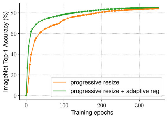
Table 13 studies our adaptive regularization on two training settings: one is to progressively increase image size from small to large (Howard, 2018), and the other is to randomly sample a different image size for each batch (Hoffer et al., 2019). Because TPU needs to recompile the graph for each new size, here we randomly sample a image size every eight epochs instead of every batch. Compared to the vanilla approaches of progressive or random resizing that use the same regularization for all image sizes, our adaptive regularization improves the accuracy by 0.7%. Figure 6 further compares the training curve for the progressive approach. Our adaptive regularization uses much smaller regularization for small images at the early training epochs, allowing models to converge faster and achieve better final accuracy.
7 Conclusion
This paper presents EfficientNetV2, a new family of smaller and faster neural networks for image recognition. Optimized with training-aware NAS and model scaling, our EfficientNetV2 significantly outperforms previous models, while being much faster and more efficient in parameters. To further speed up the training, we propose an improved method of progressive learning, that jointly increases image size and regularization during training. Extensive experiments show our EfficientNetV2 achieves strong results on ImageNet, and CIFAR/Flowers/Cars. Compared to EfficientNet and more recent works, our EfficientNetV2 trains up to 11x faster while being up to 6.8x smaller.
Acknowledgements
Special thanks to Lucas Sloan for helping open sourcing. We thank Ruoming Pang, Sheng Li, Andrew Li, Hanxiao Liu, Zihang Dai, Neil Houlsby, Ross Wightman, Jeremy Howard, Thang Luong, Daiyi Peng, Yifeng Lu, Da Huang, Chen Liang, Aravind Srinivas, Irwan Bello, Max Moroz, Futang Peng for their feedback.
References
- Bello (2021) Bello, I. Lambdanetworks: Modeling long-range interactions without attention. ICLR, 2021.
- Bello et al. (2021) Bello, I., Fedus, W., Du, X., Cubuk, E. D., Srinivas, A., Lin, T.-Y., Shlens, J., and Zoph, B. Revisiting resnets: Improved training and scaling strategies. arXiv preprint arXiv:2103.07579, 2021.
- Bengio et al. (2009) Bengio, Y., Louradour, J., Collobert, R., and Weston, J. Curriculum learning. ICML, 2009.
- Brock et al. (2021) Brock, A., De, S., Smith, S. L., and Simonyan, K. High-performance large-scale image recognition without normalization. arXiv preprint arXiv:2102.06171, 2021.
- Brown et al. (2020) Brown, T. B., Mann, B., Ryder, N., Subbiah, M., Kaplan, J., Dhariwal, P., Neelakantan, A., Shyam, P., Sastry, G., Askell, A., Agarwal, S., Herbert-Voss, A., Krueger, G., Henighan, T., Child, R., Ramesh, A., Ziegler, D. M., Wu, J., Winter, C., Hesse, C., Chen, M., Sigler, E., Litwin, M., Gray, S., Chess, B., Clark, J., Berner, C., McCandlish, S., Radford, A., Sutskever, I., and Amodei, D. Language models are few-shot learners. NeurIPS, 2020.
- Cai et al. (2019) Cai, H., Zhu, L., and Han, S. Proxylessnas: Direct neural architecture search on target task and hardware. ICLR, 2019.
- Chen et al. (2019) Chen, Y., Yang, T., Zhang, X., Meng, G., Pan, C., and Sun, J. Detnas: Neural architecture search on object detection. NeurIPS, 2019.
- Cubuk et al. (2020) Cubuk, E. D., Zoph, B., Shlens, J., and Le, Q. V. Randaugment: Practical automated data augmentation with a reduced search space. ECCV, 2020.
- Dong et al. (2020) Dong, X., Tan, M., Yu, A. W., Peng, D., Gabrys, B., and Le, Q. V. Autohas: Efficient hyperparameter and architecture search. arXiv preprint arXiv:2006.03656, 2020.
- Dosovitskiy et al. (2021) Dosovitskiy, A., Beyer, L., Kolesnikov, A., Weissenborn, D., Zhai, X., Unterthiner, T., Dehghani, M., Minderer, M., Heigold, G., Gelly, S., Uszkoreit, J., and Houlsby, N. An image is worth 16x16 words: Transformers for image recognition at scale. ICLR, 2021.
- Elsken et al. (2019) Elsken, T., Metzen, J. H., and Hutter, F. Neural architecture search: A survey. Journal of Machine Learning Research, 2019.
- Gupta & Akin (2020) Gupta, S. and Akin, B. Accelerator-aware neural network design using automl. On-device Intelligence Workshop in SysML, 2020.
- Gupta & Tan (2019) Gupta, S. and Tan, M. Efficientnet-edgetpu: Creating accelerator-optimized neural networks with automl. https://ai.googleblog.com/2019/08/efficientnet-edgetpu-creating.html, 2019.
- He et al. (2016) He, K., Zhang, X., Ren, S., and Sun, J. Deep residual learning for image recognition. CVPR, pp. 770–778, 2016.
- Hoffer et al. (2019) Hoffer, E., Weinstein, B., Hubara, I., Ben-Nun, T., Hoefler, T., and Soudry, D. Mix & match: training convnets with mixed image sizes for improved accuracy, speed and scale resiliency. arXiv preprint arXiv:1908.08986, 2019.
- Howard (2018) Howard, J. Training imagenet in 3 hours for 25 minutes. https://www.fast.ai/2018/04/30/dawnbench-fastai/, 2018.
- Huang et al. (2016) Huang, G., Sun, Y., Liu, Z., Sedra, D., and Weinberger, K. Q. Deep networks with stochastic depth. ECCV, pp. 646–661, 2016.
- Huang et al. (2017) Huang, G., Liu, Z., Van Der Maaten, L., and Weinberger, K. Q. Densely connected convolutional networks. CVPR, 2017.
- Huang et al. (2019) Huang, Y., Cheng, Y., Chen, D., Lee, H., Ngiam, J., Le, Q. V., and Chen, Z. Gpipe: Efficient training of giant neural networks using pipeline parallelism. NeurIPS, 2019.
- Karras et al. (2018) Karras, T., Aila, T., Laine, S., and Lehtinen, J. Progressive growing of gans for improved quality, stability, and variation. ICLR, 2018.
- Kolesnikov et al. (2020) Kolesnikov, A., Beyer, L., Zhai, X., Puigcerver, J., Yung, J., Gelly, S., and Houlsby, N. Big transfer (bit): General visual representation learning. ECCV, 2020.
- Krause et al. (2013) Krause, J., Deng, J., Stark, M., and Fei-Fei, L. Collecting a large-scale dataset of fine-grained cars. Second Workshop on Fine-Grained Visual Categorizatio, 2013.
- Krizhevsky & Hinton (2009) Krizhevsky, A. and Hinton, G. Learning multiple layers of features from tiny images. Technical Report, 2009.
- Li et al. (2021) Li, S., Tan, M., Pang, R., Li, A., Cheng, L., Le, Q., and Jouppi, N. Searching for fast model families on datacenter accelerators. CVPR, 2021.
- Liu et al. (2019) Liu, C., Chen, L.-C., Schroff, F., Adam, H., Hua, W., Yuille, A., and Fei-Fei, L. Auto-deeplab: Hierarchical neural architecture search for semantic image segmentation. CVPR, 2019.
- Mahajan et al. (2018) Mahajan, D., Girshick, R., Ramanathan, V., He, K., Paluri, M., Li, Y., Bharambe, A., and van der Maaten, L. Exploring the limits of weakly supervised pretraining. arXiv preprint arXiv:1805.00932, 2018.
- Nilsback & Zisserman (2008) Nilsback, M.-E. and Zisserman, A. Automated flower classification over a large number of classes. ICVGIP, pp. 722–729, 2008.
- Press et al. (2021) Press, O., Smith, N. A., and Lewis, M. Shortformer: Better language modeling using shorter inputs. arXiv preprint arXiv:2012.15832, 2021.
- Radosavovic et al. (2020) Radosavovic, I., Kosaraju, R. P., Girshick, R., He, K., and Dollár, P. Designing network design spaces. CVPR, 2020.
- Ridnik et al. (2020) Ridnik, T., Lawen, H., Noy, A., Baruch, E. B., Sharir, G., and Friedman, I. Tresnet: High performance gpu-dedicated architecture. arXiv preprint arXiv:2003.13630, 2020.
- Russakovsky et al. (2015) Russakovsky, O., Deng, J., Su, H., Krause, J., Satheesh, S., Ma, S., Huang, Z., Karpathy, A., Khosla, A., Bernstein, M., et al. Imagenet large scale visual recognition challenge. International Journal of Computer Vision, 115(3):211–252, 2015.
- Sandler et al. (2018) Sandler, M., Howard, A., Zhu, M., Zhmoginov, A., and Chen, L.-C. Mobilenetv2: Inverted residuals and linear bottlenecks. CVPR, 2018.
- Sifre (2014) Sifre, L. Rigid-motion scattering for image classification. Ph.D. thesis section 6.2, 2014.
- Srinivas et al. (2021) Srinivas, A., Lin, T.-Y., Parmar, N., Shlens, J., Abbeel, P., and Vaswani, A. Bottleneck transformers for visual recognition. arXiv preprint arXiv:2101.11605, 2021.
- Srivastava et al. (2014) Srivastava, N., Hinton, G., Krizhevsky, A., Sutskever, I., and Salakhutdinov, R. Dropout: a simple way to prevent neural networks from overfitting. The Journal of Machine Learning Research, 15(1):1929–1958, 2014.
- Tan & Le (2019a) Tan, M. and Le, Q. V. Efficientnet: Rethinking model scaling for convolutional neural networks. ICML, 2019a.
- Tan & Le (2019b) Tan, M. and Le, Q. V. Mixconv: Mixed depthwise convolutional kernels. BMVC, 2019b.
- Tan et al. (2019) Tan, M., Chen, B., Pang, R., Vasudevan, V., and Le, Q. V. Mnasnet: Platform-aware neural architecture search for mobile. CVPR, 2019.
- Tan et al. (2020) Tan, M., Pang, R., and Le, Q. V. Efficientdet: Scalable and efficient object detection. CVPR, 2020.
- Touvron et al. (2019) Touvron, H., Vedaldi, A., Douze, M., and Jégou, H. Fixing the train-test resolution discrepancy. arXiv preprint arXiv:1906.06423, 2019.
- Touvron et al. (2020) Touvron, H., Vedaldi, A., Douze, M., and Jégou, H. Fixing the train-test resolution discrepancy: Fixefficientnet. arXiv preprint arXiv:2003.08237, 2020.
- Touvron et al. (2021) Touvron, H., Cord, M., Douze, M., Massa, F., Sablayrolles, A., and Jégou, H. Training data-efficient image transformers & distillation through attention. arXiv preprint arXiv:2012.12877, 2021.
- Wightman (2021) Wightman, R. Pytorch image model. https://github.com/rwightman/pytorch-image-models, Accessed on Feb.18, 2021, 2021.
- Wu et al. (2019) Wu, B., Dai, X., Zhang, P., Wang, Y., Sun, F., Wu, Y., Tian, Y., Vajda, P., Jia, Y., and Keutzer, K. Fbnet: Hardware-aware efficient convnet design via differentiable neural architecture search. CVPR, 2019.
- Xie et al. (2020) Xie, Q., Luong, M.-T., Hovy, E., and Le, Q. V. Self-training with noisy student improves imagenet classification. CVPR, 2020.
- Xiong et al. (2020) Xiong, Y., Liu, H., Gupta, S., Akin, B., Bender, G., Kindermans, P.-J., Tan, M., Singh, V., and Chen, B. Mobiledets: Searching for object detection architectures for mobile accelerators. arXiv preprint arXiv:2004.14525, 2020.
- Yu et al. (2019) Yu, H., Liu, A., Liu, X., Li, G., Luo, P., Cheng, R., Yang, J., and Zhang, C. Pda: Progressive data augmentation for general robustness of deep neural networks. arXiv preprint arXiv:1909.04839, 2019.
- Yuan et al. (2021) Yuan, L., Chen, Y., Wang, T., Yu, W., Shi, Y., Tay, F. E., Feng, J., and Yan, S. Tokens-to-token vit: Training vision transformers from scratch on imagenet. arXiv preprint arXiv:2101.11986, 2021.
- Zhang et al. (2018) Zhang, H., Cisse, M., Dauphin, Y. N., and Lopez-Paz, D. Mixup: Beyond empirical risk minimization. ICLR, 2018.
- Zhang et al. (2020) Zhang, H., Wu, C., Zhang, Z., Zhu, Y., Lin, H., Zhang, Z., Sun, Y., He, T., Mueller, J., Manmatha, R., Li, M., and Smola, A. Resnest: Split-attention networks. arXiv preprint arXiv:2012.12877, 2020.
- Zoph et al. (2018) Zoph, B., Vasudevan, V., Shlens, J., and Le, Q. V. Learning transferable architectures for scalable image recognition. CVPR, 2018.