KMT-2019-BLG-1715: planetary microlensing event with three lens masses and two source stars

Abstract

We investigate the gravitational microlensing event KMT-2019-BLG-171, of which light curve shows two short-term anomalies from a caustic-crossing binary-lensing light curve: one with a large deviation and the other with a small deviation. We identify five pairs of solutions, in which the anomalies are explained by adding an extra lens or source component in addition to the base binary-lens model. We resolve the degeneracies by applying a method, in which the measured flux ratio between the first and second source stars is compared with the flux ratio deduced from the ratio of the source radii. Applying this method leaves a single pair of viable solutions, in both of which the major anomaly is generated by a planetary-mass third body of the lens, and the minor anomaly is generated by a faint second source. A Bayesian analysis indicates that the lens comprises three masses: a planet-mass object with $\sim 2.6~{}M_{\rm J}$ and binary stars of K and M dwarfs lying in the galactic disk. We point out the possibility that the lens is the blend, and this can be verified by conducting high-resolution followup imaging for the resolution of the lens from the source.

1. Introduction

During the first-generation experiment (Udalski et al., 1994a; Alcock et al, 1997), microlensing observations were carried out with about one day cadence. By employing wide-field cameras mounted on multiple telescopes, the cadence of microlensing observations has been dramatically shortened, and now it reaches 15 minutes for the fields of the highest stellar concentration. With the shortened cadence, the event detection rate has greatly increased from several dozens/yr during the first-generation experiments to the current rate of more than 3000 events/yr.

Light curves of lensing events often deviate from that of a single lens and a single source (1L1S) event, which produces a smooth and symmetric light curve. The most common cause of the deviation is the binarity of the lens: 2L1S events (Mao & Paczyński, 1991). Interpreting the light curves of 2L1S events was a challenging task at the time when such events were first detected, e.g., OGLE No. 7 (Udalski et al., 1994b), because the methodology for the analysis of these anomalous events had not yet been developed. With the development of various methodologies, e.g., ray-shooting technique (Bond et al., 2002; Dong et al., 2009; Bennett, 2010) and contour integration algorithm (Gould & Gaucherel, 1997; Bozza et al., 2018) developed for finite magnification computations, followed by the theoretical understanding of the binary lensing physics, 2L1S events are routinely detected and analyzed as they progress (Ryu et al., 2010; Bozza et al., 2012).

With the increasing number of densely covered events, one occasionally confronts events having light curves that exhibit extra deviations from those of 2L1S events. One important cause of such extra deviations is the existence of an additional lens or source component. There exist 12 confirmed events, for which at least four objects, including the lens and source components, are needed for the interpretations of the light curves. See Table 1 of Han et al. (2021). Among these events, 9 events were produced by triple lens systems, 3L1S events. For two major reasons, modeling a 3L1S event is difficult. The first is the complexity of the lensing behavior (Daněk & Heyrovský, 2015, 2019) and the resulting difficulties in analyzing deviations. Another important obstacle in analyzing these events is the degeneracy problem, which makes it difficult to find a correct solution among those resulting in similar light curves despite dramatically different interpretations of the lens system. Identifying various types of degeneracies and investigating their causes are important not only to correctly interpret the lens system but also to investigate similar degeneracies in following analyses.

We investigate the microlensing event KMT-2019-BLG-1715 and present the analysis result. The event displays a light curve with a complex pattern, in which there exist two short-lasting anomalies deviating from a caustic-crossing 2L1S light curve. We model the observed light curve under various interpretations and present the results.

The organization of the paper for the presentation of the analysis is as follows. We address the acquisition and reduction of data in Sect. 2. We depict the pattern of the anomalies that deviate from a 2L1S lensing light curve in Sect. 3. We present various models describing the anomalies in Sect. 4. We inspect the origins of the degeneracies among the identified solutions in Section 5. We characterize the source, and measure the Einstein radius in Sect. 6. We probe a method that can resolve the degeneracies in the lensing models in Sect. 7. In Sect. 8, we describe a Bayesian analysis conducted to characterize the lens, and present the physical quantifies. We summarize the analysis and make a conclusion in Sect. 9.

Table 1Data and error readjustment factors

Data set	$k$	$\sigma_{\rm min}$ (mag)	$N_{\rm data}$
OGLE	1.225	0.030	450
KMTA (BLG03)	1.404	0.020	1307
KMTA (BLG43)	0.812	0.050	1195
KMTA (BLG03)	1.517	0.010	1109
KMTA (BLG43)	1.217	0.020	1424
KMTC (BLG03)	1.382	0.010	981
KMTS (BLG43)	1.187	0.020	1314

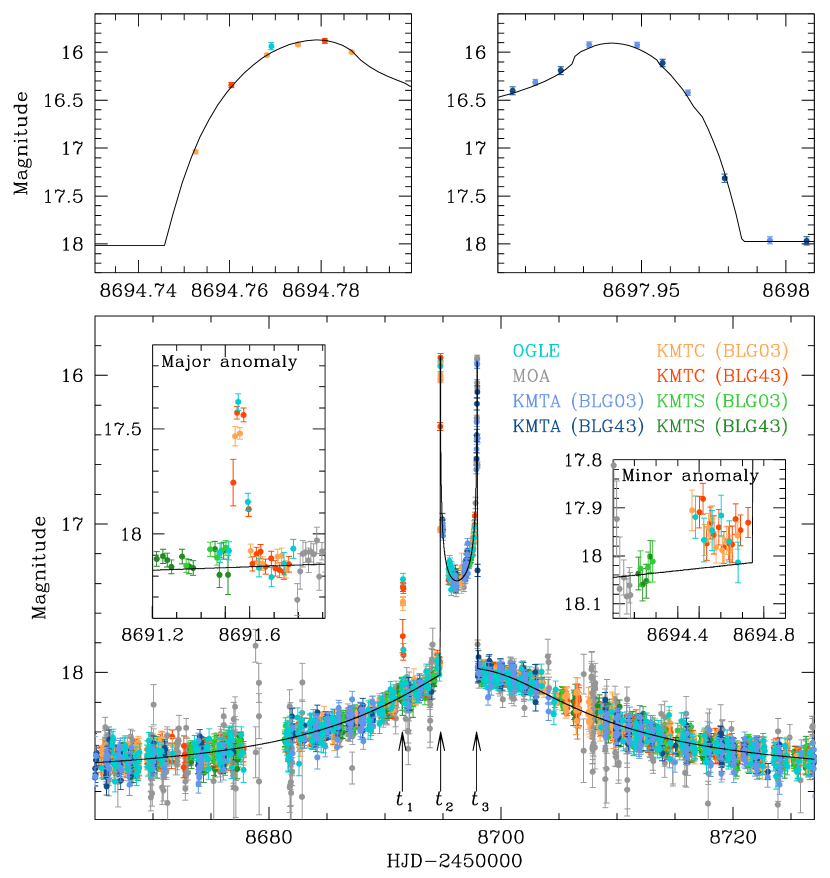
Figure 1.— Lensing light curve of KMT-2019-BLG-1715. The model obtained from a 2L1S interpretation (close model) is drawn over the data points. The two top panels show the zoom-in views around the times of the source star’s entrance into and exit from the caustic according to the 2L1S model. The two insets in the lower panel show the zoomed-in views around the two anomalies from the 2L1S model occurred at ${\rm HJD}^{\prime}\sim 8691.5$ (major anomaly) and $\sim 8694.5$ (minor anomaly).

2. Observations and Data

The event KMT-2019-BLG-1715 was found from the observations of a source star lying at $({\rm RA},{\rm DEC})_{\rm J2000}=(18:01:29.21,-28:46:37.7)$, that correspond to $(l,b)=(1^{\circ}\hskip-2.0pt.898,-2^{\circ}\hskip-2.0pt.914)$. The apparent source magnitude at the baseline was $I_{\rm base}=18.65$.

The magnification of the source flux was discovered from the Korea Microlensing Telescope Network (KMTNet: Kim et al., 2016) survey on 2019 July 20 (${\rm HJD}^{\prime}\equiv{\rm HJD}-2450000\sim 8684.7$), at which the source became brighter by about $0.25$ magnitude from the baseline. The KMTNet survey utilizes three telescopes that lie around the world in Australia (KMTA), Chile (KMTC), and South Africa (KMTS). The aperture of each telescope is 1.6 meter, and the field of view of the camera mounted on the telescope is $4~{}{\rm deg}^{2}$. The source lies in the BLG03 and BLG43 fields, which overlap with a small offset, and thus the data are composed of six sets, with two sets from each telescope.

The event was independently found by two other lensing surveys of the Optical Gravitational Lensing Experiment (OGLE: Udalski et al., 2015) and the Microlensing Observations in Astrophysics (MOA: Bond et al., 2001) on 2019 July 28 (${\rm HJD}^{\prime}\sim 8692.7$) and August 1 (${\rm HJD}^{\prime}\sim 8696.7$), respectively. The OGLE and MOA surveys designated the event as OGLE-2019-BLG-1190 and MOA-2019-BLG-352, respectively. The OGLE survey uses the 1.3 m Warsaw Telescope located at the Las Campanas Observatory in Chile, and the MOA survey utilizes the 1.8 m MOA-II Telescope located at Mt. John Observatory in New Zealand.

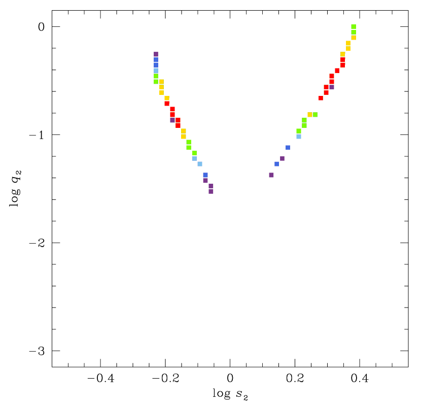
Figure 2.— Distribution of $\Delta\chi^{2}$ on the $\log s$–$\log q$ plane. Red, yellow, green, cyan, blue, and purple colors are used to designate points with $<1n\sigma$, $<2n\sigma$, $<3n\sigma$, $<4n\sigma$, $<5n\sigma$, and $<6n\sigma$, where $n=10$.

The data were processed utilizing the photometry pipelines of the individual groups: Albrow (2017), Udalski (2003), and Bond et al. (2001) for the KMTNet, OGLE, and MOA surveys, respectively. We note that these pipelines commonly utilize the difference imaging algorithm that was developed to optimize photometry in very crowded fields (Alard & Lupton, 1998). Although the MOA data cover the caustic crossing at ${\rm HJD}^{\prime}\sim 8697.9$, which is also densely covered by the KMTA data sets, they do not cover the anomalies of our major interest to be discussed below. Furthermore, the photometric uncertainties of the data are substantially larger than those of the other data sets, and thus the MOA data are not used for analysis to minimize their effects on modeling. The error bars of the data used in the analysis were rescaled from those estimated from the automatized pipelines, $\sigma_{0}$, by $\sigma=k(\sigma_{\rm min}^{2}+\sigma_{0}^{2})^{1/2}$, where $k$ denotes a rescaling factor to normalize $\chi^{2}/{\rm dof}$, where dof represents the degree of freedom, to unity, and $\sigma_{\rm min}$ is the scatter of data (Yee et al., 2012). In Table 1, we list $(k,\sigma_{\rm min},N_{\rm data})$ for the six data sets. Here $N_{\rm data}$ denotes the number of data in each data set.

Table 2Lensing parameters of 2L1S model

Parameter	Close	Wide
$\chi^{2}$	9329.3	9313.7
$t_{0}$ (${\rm HJD}^{\prime}$)	$8697.039\pm 0.022$	$8696.971\pm 0.016$
$u_{0}$	$0.123\pm 0.002$	$0.091\pm 0.001$
$t_{\rm E}$ (days)	$30.94\pm 0.31$	$39.04\pm 0.35$
$s$	$0.756\pm 0.006$	$2.028\pm 0.002$
$q$	$0.141\pm 0.002$	$0.310\pm 0.006$
$\alpha$ (rad)	$4.945\pm 0.005$	$4.913\pm 0.005$
$\rho$ ($10^{-3}$)	$0.65\pm 0.01$	$0.57\pm 0.01$

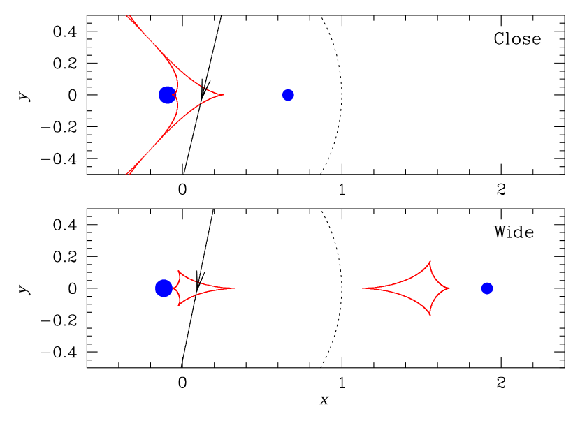
Figure 3.— Lensing configurations of the two 2L1S models. The blue dots indicate the lens positions, the red figures represent the caustics, and the arrowed line represents the source motion. The Einstein ring is marked by a dotted circle.

3. 2L1S interpretation

The observed light curve of KMT-2019-BLG-1715 is shown in Figure 1. At first glance, the two pronounced caustic-crossing spikes, at ${\rm HJD}^{\prime}\sim 8694.7$ ($t_{2}$) and $\sim 8697.9$ ($t_{3}$), suggests that the event is a usual caustic-crossing 2L1S event. Fitting the light curve with a 2L1S model yields a pair of solutions with $(s,q)\sim(0.76,0.14)$ (“close” model) and $(s,q)\sim(2.03,0.31)$ (“wide” model), where $s$ and $q$ denote the projected separation (scaled to the Einstein radius $\theta_{\rm E}$) and the mass ratio between the binary lens components, with masses $M_{1}$ and $M_{2}$, respectively. We carry out the 2L1S modeling in two steps, in which the binary parameters $(s,q)$ are searched for via a dense grid approach in the first step, and locals appearing in the $\Delta\chi^{2}$ map are refined in the second step. The ranges of the grid parameters are $-1.0\leq\log s\leq 1.0$ and $-3.0\leq\log q\leq 0.0$ with 60 divisions. Figure 2 shows the $\Delta\chi^{2}$ distribution obtained from the grid search and the locations of the two locals, i.e., close and wide solutions.

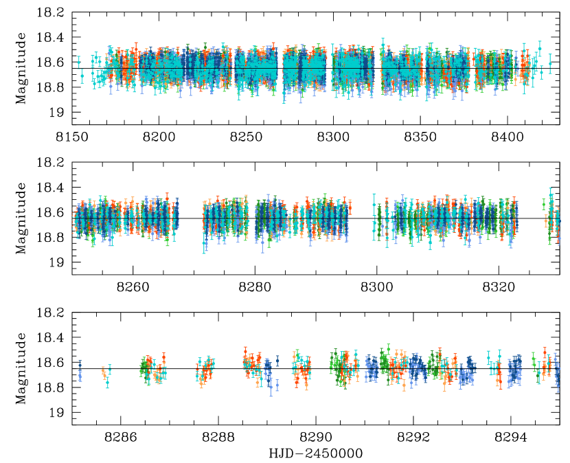
Figure 4.— Light curves at the baseline during three different time spans: 280 days (top panel), 80 days (middle panel), and 10 days (bottom panel). The colors of data points are same as those in Fig. 1.

We list the full lensing parameters of the two 2L1S solutions in Table 2. In the table, the parameters $(t_{0},u_{0},t_{\rm E})$ denote the closest source approach time to a lens reference position, the reference-source separation at $t_{0}$, and the timescale of the event, respectively. As a lens reference, we choose the center of mass for a close binary ($s<1.0$), and the effective lens position, defined by Di Stefano & Mao (1996) and An & Han (2002), for a wide binary ($s>1.0$). Because the light curve exhibits pronounced caustic-crossing spikes, finite-source effects (hereafter “finite effects”) are considered in modeling by including $\rho=\theta_{*}/\theta_{\rm E}$ (normalized “source radius”) as an additional parameter. Here $\theta_{*}$ denote the angular source radius. Hereafter, we denote $\theta_{*}$ and $\theta_{\rm E}$ without the notation of “angular”. In the computation of finite magnifications, we take limb-darkening effects into consideration assuming that the brightness profile on the source surface varies as $\Sigma_{\lambda}\propto 1-(1-3\cos\phi/2)\Gamma_{\lambda}$. Here $\Gamma_{\lambda}$ denotes the coefficient of limb darkening, and $\phi$ denotes the angle between the two lines extending from the source center, one toward an observer and the other toward the source surface. Based on the spectral type, to be discussed in Section 6, we adopt the $V$- and $I$-band coefficients of $(\Gamma_{V},\Gamma_{I})=(0.62,0.45)$. The two solutions (close and wide) are degenerate, and the degeneracy is originated from the close–wide degeneracy known by Dominik (1999). The lensing configurations, showing the trajectory of the source relative to the lens components and caustic, are provided in Figure 3. The model curve of the 2L1S solution (for the close model) is shown in Figure 1.

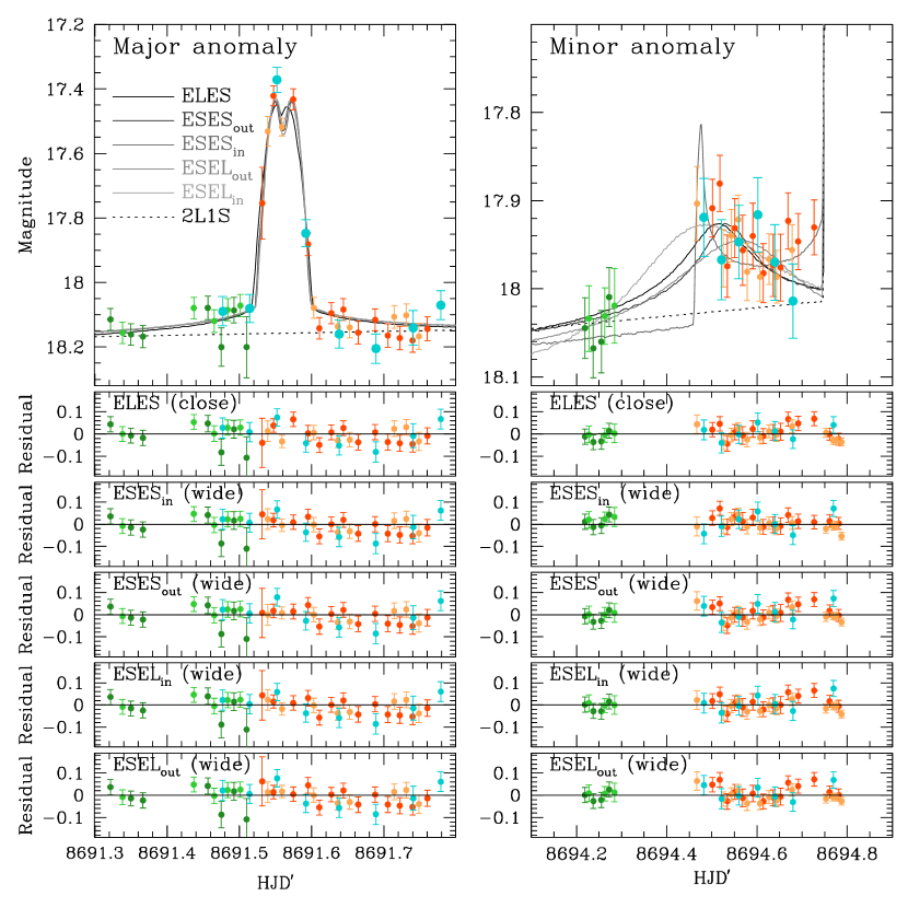
Figure 5.— Zoomed-in views of the light curve around the major (at around $t_{1}$) and minor (at around $t_{2}$) anomalies. For each epoch, the lower five panels show the residuals from the identified five sets of degenerate solutions: ELES (close), ESES_in (wide), ESEL_out (wide), ESEL_in (wide), and ESEL_out (wide) solutions. For each set, there are two solutions with $s_{2}<1.0$ (close) and $s_{2}>1.0$ (wide), and the presented residuals are for the solution yielding a better fit among the close–wide solutions. Drawn over the data points are models of five degenerate solutions. The degeneracies among the solutions are severe, resulting in similar model curves. The only significant difference is the extra caustic entrance at $t_{2}$ corresponding to the ESES_in model.

Although the 2L1S model approximately describes the overall features of the observed light curve, a close look reveals that the data exhibit two short-lasting anomalies from the base 2L1S model. The first anomaly appears at ${\rm HJD}^{\prime}\sim 8691.5$ ($t_{1}$) with $\Delta I\sim 0.7$ mag deviation from the 2L1S model. The second anomaly appears just before the second caustic crossing at $\sim 8694.5$ ($t_{2}$) with $\Delta I\sim 0.1$ mag deviation. We refer to the former and latter anomalies as the “major anomaly” and “minor anomaly”, respectively. The two insets in the lower panel of Figure 1 show the zoom-in views of the anomalies. The major anomaly exhibits both rising and falling parts during its very short duration of $\sim 3$ hours. The duration of the minor anomaly is short as well, but precisely estimating the duration is difficult because the coverage of the anomaly is incomplete.

We check the possibility that the extra anomalies arise due to photometric artifacts or stellar variability. First, the possibility of the photometric artifact, such as the change in transparency or the passage of a Solar System object across the source, is very unlikely because both anomalies are covered by multiple remotely separated telescopes and the data during the anomalies show consistent patterns of variations. Second, the possibility of the source variability is also unlikely because the stellar type of the source is a main sequence, for which the chance of light variation is very small. We check the source variability by inspecting the light curve at the baseline. Figure 4 shows the baseline light curve during three different time spans: 280 days (top panel), 80 days (middle panel), and 10 days (bottom panel). It is found that the light curve does not show any variation in all inspected time ranges.

Table 3Lensing parameters of ESES models

Parameter	ESESin		ESESout
	Close	Wide	Close	Wide
$\chi^{2}$	7737.0	7696.1	7771.2	7701.1
$t_{0,1}$ (${\rm HJD}^{\prime}$)	$8697.047\pm 0.019$	$8697.153\pm 0.017$	$8697.046\pm 0.015$	$8697.113\pm 0.016$
$u_{0,1}$	$0.103\pm 0.002$	$0.107\pm 0.001$	$0.102\pm 0.001$	$0.096\pm 0.001$
$t_{0,2}$ (${\rm HJD}^{\prime}$)	$8693.518\pm 0.035$	$8694.716\pm 0.059$	$8693.525\pm 0.029$	$8694.400\pm 0.052$
$u_{0,2}$	$0.205\pm 0.002$	$0.368\pm 0.002$	$0.204\pm 0.002$	$0.304\pm 0.002$
$t_{0,3}$ (${\rm HJD}^{\prime}$)	$8696.383\pm 0.037$	$8697.270\pm 0.058$	$8696.669\pm 0.047$	$8697.865\pm 0.105$
$u_{0,3}$	$0.188\pm 0.003$	$0.309\pm 0.003$	$0.222\pm 0.003$	$0.357\pm 0.007$
$t_{\rm E}$ (days)	$32.58\pm 0.28$	$35.43\pm 0.17$	$32.66\pm 0.05$	$37.31\pm 0.25$
$s$	$0.696\pm 0.004$	$1.988\pm 0.001$	$0.693\pm 0.003$	$2.078\pm 0.003$
$q$	$0.177\pm 0.003$	$0.349\pm 0.004$	$0.178\pm 0.002$	$0.385\pm 0.007$
$\alpha$ (rad)	$4.997\pm 0.005$	$4.950\pm 0.004$	$4.999\pm 0.004$	$4.957\pm 0.005$
$\rho_{1}$ ($10^{-3}$)	$0.59\pm 0.01$	$0.63\pm 0.01$	$0.60\pm 0.01$	$0.58\pm 0.01$
$\rho_{2}$ ($10^{-3}$)	$0.47\pm 0.04$	$0.45\pm 0.04$	$0.42\pm 0.04$	$0.43\pm 0.04$
$\rho_{3}$ ($10^{-3}$)	–	–	–	–
$q_{F,2}$	$0.051\pm 0.002$	$0.060\pm 0.002$	$0.050\pm 0.001$	$0.059\pm 0.002$
$q_{F,3}$	$0.020\pm 0.003$	$0.021\pm 0.003$	$0.029\pm 0.004$	$0.040\pm 0.006$

4. Interpreting the anomalies

We investigate lensing models that can explain the observed anomalies from the 2L1S models. From this investigation, we find that adding a fourth body (either a source or a lens) can explain one of the two anomalies, but not both simultaneously. Solutions explaining both anomalies can only be found from combinations of an extra lens (EL) and an extra source (ES), and we find five sets of such solutions resulting from various types of degeneracy. For each set, there exist two solutions with $s_{2}>1.0$ and $s_{2}<1.0$ resulting from the close–wide binary degeneracy, and thus there are ten solutions in total. The details of the individual models are discussed in the following subsections.

For the designation of the individual solutions to be discussed, we use the notations “ELES” (extra lens and extra source), “ESES” (extra source and extra source), and “ESEL” (extra source and extra lens). In these notations, the first “L” (or “S”) indicates that an extra lens (an extra source) is included in the model to explain the major anomaly, while the second “L” (or “S”) denotes that an extra lens (or source) is included to describe the minor anomaly. For example, “ELES” denotes a model, in which the major and minor anomalies are explained by adding an extra lens and an extra source to the base 2L1S solution, respectively, and thus the model consists of three lens components and two source stars.

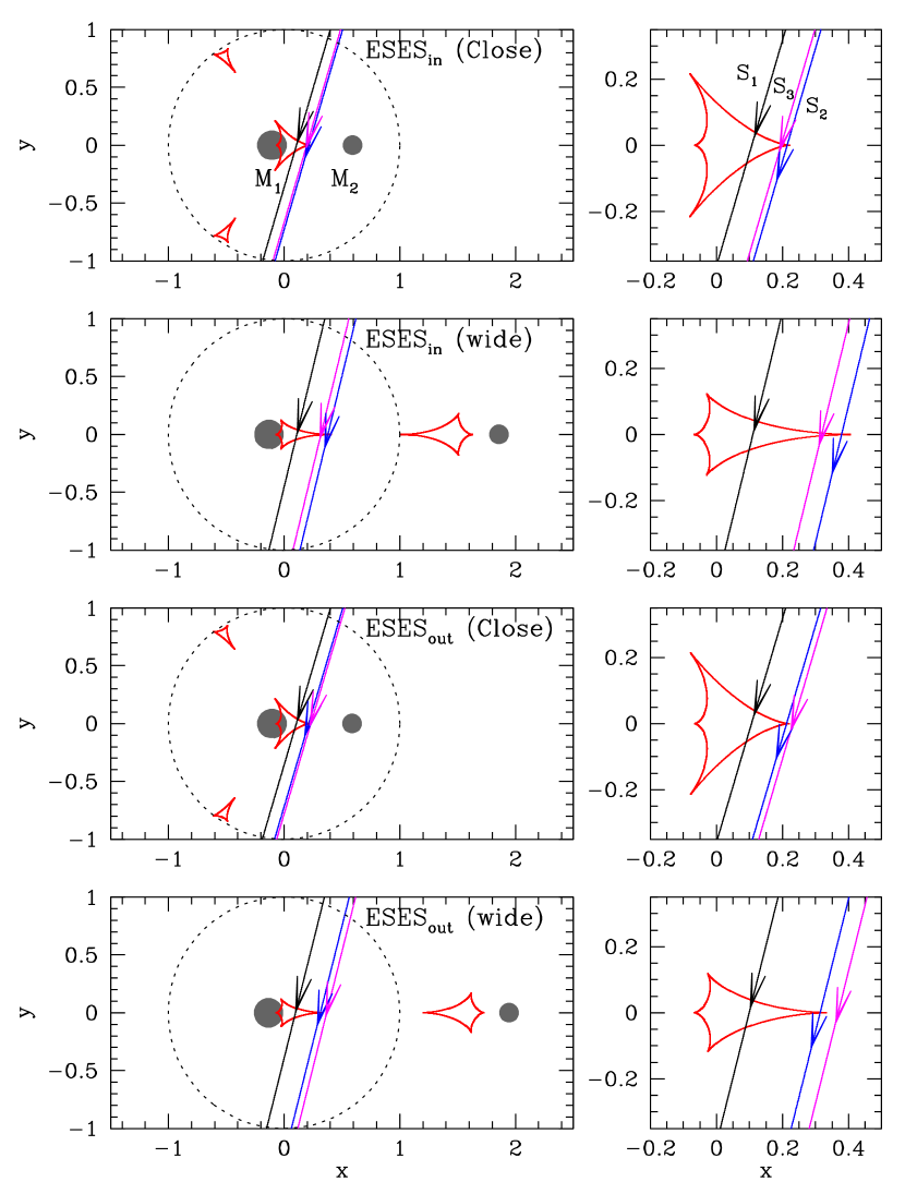
Figure 6.— Lensing configurations for the four ESES models: ESES_in (close), ESES_in (wide), ESES_out (close), and ESES_out (wide). For each solution, the panel on the left shows the wide view including the lens positions, and the panel on the right shows the central region. The positions of the lens components are marked by two filled dots ($M_{1}$ and $M_{2}$). The three lines with arrows denote the motion of the primary ($S_{1}$, black), second ($S_{1}$, blue), and third ($S_{1}$, magenta) source stars.

4.1. ESES solutions

The ESES solutions explain both the major and minor anomalies with the addition of two extra source stars to the base 2L1S model. In the modeling considering additional source stars, the initial lensing parameters related to the first source are adopted from those of the 2L1S model, and the initial parameters related to the other source stars are assigned considering the locations and magnitudes of the anomalies. According to these solutions, then, there are two lens masses ($M_{1}$ and $M_{2}$) and three source stars ($S_{1}$, $S_{2}$, and $S_{3}$): 2L3S model. Besides the close-wide degeneracy, the ESES interpretation additionally suffers from a degeneracy arising due to the ambiguity in the trajectory of $S_{3}$, resulting in four degenerate solutions in total. The two sets of the degenerate solutions resulting from the latter type degeneracy, ESES_in and ESES_out, commonly explain the origin of the major anomaly as the second source ($S_{2}$) star’s caustic crossing over the tip of the binary-induced caustic. According to the ESES_in and ESES_out solutions, the tertiary source ($S_{3}$) star, that is introduced to explain the minor anomaly, passes the inner and outer region of the caustic, respectively. The degeneracy between the two solutions results from the incomplete coverage of the minor anomaly.

Table 4Lensing parameters of ESEL models

Parameter	ESELin		ESELout
	Close	Wide	Close	Wide
$\chi^{2}$	7713.6	7668.5	7741.3	7667.9
$t_{0,1}$ (${\rm HJD}^{\prime}$)	$8697.094\pm 0.015$	$8697.071\pm 0.016$	$8697.141\pm 0.014$	$8697.023\pm 0.015$
$u_{0,1}$	$0.109\pm 0.002$	$0.092\pm 0.001$	$0.121\pm 0.001$	$0.078\pm 0.002$
$t_{0,2}$ (${\rm HJD}^{\prime}$)	$8693.547\pm 0.034$	$8694.239\pm 0.057$	$8693.599\pm 0.033$	$8693.982\pm 0.066$
$u_{0,2}$	$0.216\pm 0.003$	$0.292\pm 0.004$	$0.232\pm 0.002$	$0.229\pm 0.010$
$t_{\rm E}$ (days)	$32.05\pm 0.39$	$38.35\pm 0.34$	$30.57\pm 0.28$	$42.92\pm 1.03$
$s_{2}$	$0.716\pm 0.004$	$2.089\pm 0.009$	$0.739\pm 0.003$	$2.227\pm 0.026$
$q_{2}$	$0.164\pm 0.002$	$0.372\pm 0.007$	$0.162\pm 0.002$	$0.398\pm 0.012$
$\alpha$ (rad)	$4.991\pm 0.005$	$4.947\pm 0.005$	$4.992\pm 0.005$	$4.954\pm 0.004$
$s_{3}$	$1.178\pm 0.006$	$0.952\pm 0.004$	$1.098\pm 0.003$	$0.891\pm 0.005$
$q_{3}$ ($10^{-3}$)	$0.26\pm 0.05$	$0.06\pm 0.01$	$0.05\pm 0.01$	$0.03\pm 0.01$
$\psi$ (rad)	$0.734\pm 0.004$	$0.902\pm 0.003$	$0.711\pm 0.003$	$0.929\pm 0.005$
$\rho_{1}$ ($10^{-3}$)	$0.62\pm 0.01$	$0.57\pm 0.01$	$0.65\pm 0.01$	$0.50\pm 0.02$
$\rho_{2}$ ($10^{-3}$)	$0.52\pm 0.04$	$0.43\pm 0.04$	$0.48\pm 0.04$	$0.34\pm 0.04$
$q_{F}$	$0.052\pm 0.002$	$0.059\pm 0.002$	$0.049\pm 0.002$	$0.057\pm 0.002$

The lensing configurations of the four ESES solutions are presented in Figure 6, in which the trajectories of the second and third source stars are marked by $S_{2}$, and $S_{3}$, respectively. The model curves and residuals from the models in the regions around the anomalies are shown in Figure 5. We note that the presented models are the wide solutions, which yield better fits than the corresponding close solutions. The minor anomaly according to the ESES_in solution is characterized by a U-shape trough pattern because $S_{3}$ passes the inner region of the caustic. The lensing parameters of the ESES_in and ESES_out, including both the close and wide solutions, are listed in Table 3. The flux ratios of the secondary and tertiary source stars to the primary source are $q_{F,2}=F_{S,2}/F_{S,1}\sim 0.05$–0.06 and $q_{F,3}=F_{S,3}/F_{S,1}\sim 0.02$–0.05, respectively. Here $F_{S,i}$ and $(t_{0,i},u_{0,i},\rho_{i})$ indicate the flux and the lensing parameters related to the $i$th source star, respectively. It is found that $\rho_{3}$ cannot be firmly determined because the coverage of the minor anomaly is incomplete.

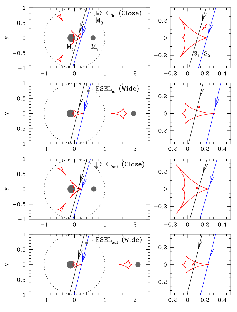
Figure 7.— Lensing configurations of the four ESEL solutions: ESEL_in (close), ESEL_in (wide), ESEL_out (close), and ESEL_out (wide). Notations are same as those in Fig. 6, except that there are three lens components ($M_{1}$, $M_{2}$, and $M_{3}$) and two source stars ($S_{1}$ and $S_{2}$).

4.2. ESEL solutions

According to the ESEL solutions, the lens and source of the event comprise three lens masses ($M_{1}$, $M_{2}$, and $M_{3}$) and two source stars ($S_{1}$ and $S_{2}$), respectively: 3L2S model. Finding solutions is carried out in two steps. In the first step, we fit the minor anomaly by adding an extra lens component: 3L1S model. Because the overall pattern of the light curve is described by a 2L1S model, the anomaly can be treated as a perturbation to the 2L1S model (Bozza, 1999; Han et al., 2001). Under this assumption, we search for a 3L1S model by fixing the parameters of the 2L1S model ($s_{2}$, $q_{2}$, and $\alpha$), and then conducting a grid search for the parameters describing the third lens component ($s_{3}$, $q_{3}$, and $\psi$). Here ($s_{3}$, $q_{3}$) are the separation and mass ratio of $M_{3}$ with respect to $M_{1}$, respectively, and $\psi$ indicates the $M_{3}$ orientation angle, which is measured from the $M_{1}$–$M_{2}$ axis in a clockwise sense centered at the position of $M_{1}$. The parameter ranges are $-1.0\leq\log s_{3}\leq 1.0$, $-5.0\leq\log q_{3}\leq 1.0$, and $0\leq\psi<2\pi$, and they are divided into 50, 50, and 180 grids, respectively. The solutions are refined by gradually narrowing down the ranges of the grid parameters, and then by releasing all parameters as free parameters. In the second step, we fit the major anomaly by introducing an extra source $S_{2}$ based on the 3L1S solution found in the first step. Adding an additional source component requires us to include additional parameters, including $(t_{0,2},u_{0,2},\rho_{2},q_{F})$, where $q_{F}$ represents the $S_{1}/S_{2}$ flux ratio.

Under the ESEL interpretation, we find four solutions, in which there exist a pair of solutions for each of the close and wide solutions. For all of these solutions, the major anomaly is generated by the crossing of $S_{2}$ over the $M_{2}$-induced caustic, and the minor anomaly is generated by the passage of $S_{1}$ through the region around the tiny $M_{3}$-induced caustic. Under this interpretation, there are two solutions, designated as ESEL_in and ESEL_out solutions, for each of the close and wide solutions. The difference between the ESEL_in and ESEL_out solutions is that the first source ($S_{1}$) passes the inner side (with respect to $M_{1}$) of the caustic induced by $M_{3}$ for the ESEL_in solution, while $S_{1}$ passes the outer side of the caustic for the ESEL_out solution. Figure 7 shows the lensing configurations of the four ESEL solutions.

The model curves of the wide ESEL_in and ESEL_out solutions around the anomalies are shown in Figure 5, and the parameters of the four ESEL solutions are listed in Table 4. We note that the mass ratio between $M_{3}$ and $M_{1}$ of the lens, $q_{3}\sim(4$–$26)\times 10^{-5}$, is very small, indicating that $M_{3}$ is a very low-mass planet according to these solutions. Due to the small mass ratio, the caustic induced by $M_{3}$ is much smaller than the caustic induced by $M_{2}$.

Table 5Lensing parameters of ELES models

Parameter	Close	Wide
$\chi^{2}$	7689.8	7713.7
$t_{0,1}$ (${\rm HJD}^{\prime}$)	$8696.722\pm 0.012$	$8696.819\pm 0.009$
$u_{0,1}$	$0.056\pm 0.001$	$0.053\pm 0.001$
$t_{0,2}$ (${\rm HJD}^{\prime}$)	$8695.773\pm 0.027$	$8696.341\pm 0.054$
$u_{0,2}$	$0.147\pm 0.001$	$0.181\pm 0.002$
$t_{\rm E}$ (days)	$43.96\pm 0.06$	$51.93\pm 0.08$
$s_{2}$	$0.551\pm 0.003$	$2.524\pm 0.001$
$q_{2}$	$0.246\pm 0.006$	$0.461\pm 0.002$
$\alpha$ (rad)	$4.894\pm 0.005$	$4.897\pm 0.005$
$s_{3}$	$1.054\pm 0.001$	$0.904\pm 0.001$
$q_{3}$ ($10^{-3}$)	$4.01\pm 0.16$	$2.30\pm 0.10$
$\psi$ (rad)	$1.348\pm 0.008$	$1.341\pm 0.006$
$\rho_{1}$ ($10^{-3}$)	$0.44\pm 0.01$	$0.41\pm 0.01$
$\rho_{2}$ ($10^{-3}$)	–	–
$q_{F}$	$0.043\pm 0.005$	$0.042\pm 0.005$

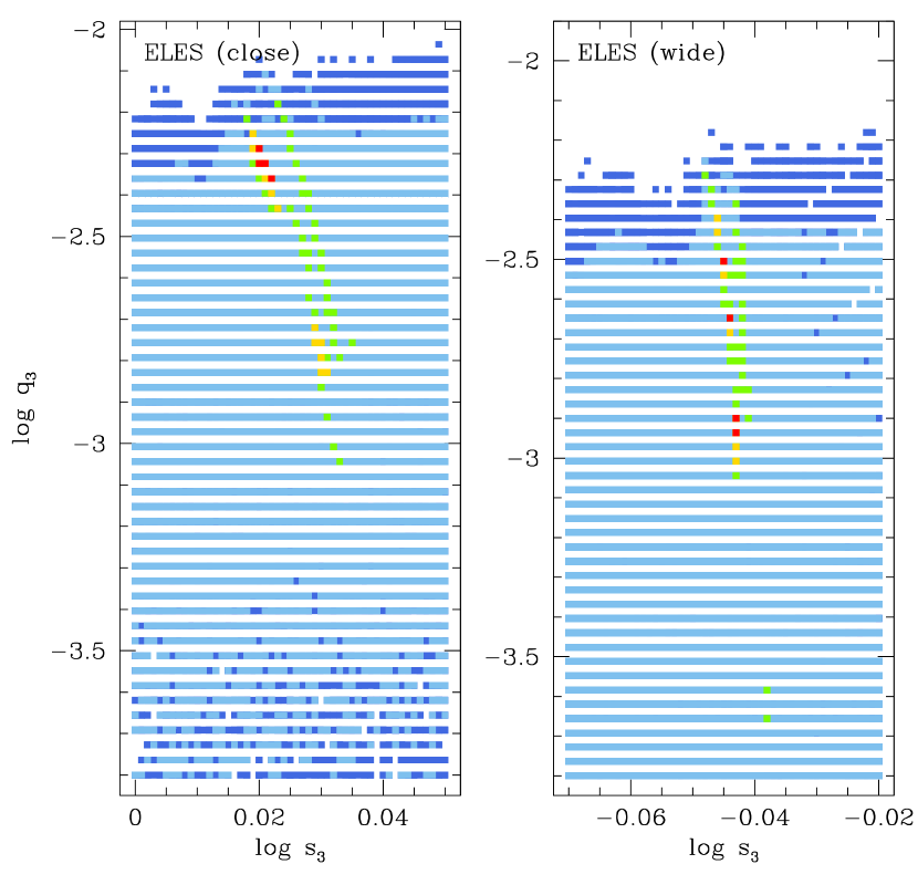
Figure 8.— $\Delta\chi^{2}$ map on the $s_{3}$–$q_{3}$ plane for the close and wide 3L1S models. The colors of points follows the same coding as in Fig. 2.

4.3. ELES solutions

We find another 3L2S solutions, in which the way of interpreting the observed anomalies is different from that of the 3L2S solutions described in the previous subsection. We find these solutions by first fitting the major anomaly from a 3L1S modeling, and then fitting the minor anomaly with the introduction of an extras source $S_{2}$. We note that the ESEL solutions, discussed in the previous subsection, are obtained by fitting the minor anomaly first from a 3L1S modeling. According to the new 3L2S solutions, the major and minor anomalies are explained with the addition of $M_{3}$ and $S_{2}$ to the baseline 2L1S model, i.e., ELES models. For each of the close and wide solutions, there is no additional degeneracy, and thus there are two ELES solutions. In Figure 8, we present the $\Delta\chi^{2}$ map on the $s_{3}$–$q_{3}$ plane.

We list the lensing parameters of the two ELES solutions (close and wide) in Table 5. The estimated mass ratio, $q_{3}\equiv M_{3}/M_{1}\sim(2$–$4)\times 10^{-3}$, is very low, suggesting that $M_{3}$ is a planetary-mass object belonging to the $M_{1}$–$M_{2}$ binary system according to the ELES model. The separation and the orientation angle of the planet from $M_{1}$ is $s_{3}\sim 1$ and $\psi=1.34$ (77.3^∘), respectively. The value of $\rho_{2}$ is not presented in the table because $S_{2}$ does not involve with caustic crossings, resulting in no finite effect.

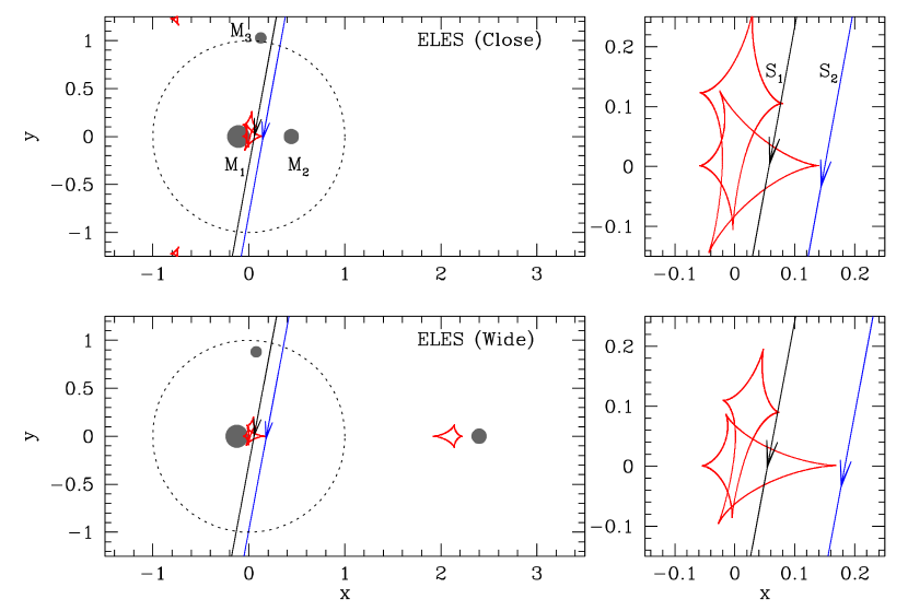
Figure 9.— Lensing configurations of the two ELES solutions: ELES (close) and ELES (wide).

The model curve and the residuals from the ELES solutions at around the times of the anomalies are shown in Figure 5. The lensing configurations are presented in Figure 9. It is found that the configuration is greatly different from that of ESEL solutions, although the lens systems of both ESEL and ELES solutions constitute the same numbers of the lens and source components, i.e., 3L2S model. We note that the caustics exhibit a self-intersecting pattern, which is a characteristic pattern of a 3L system (Gaudi et al., 1998). From the comparison of the lensing configurations with that of the 2L1S model (shown in Figure 3), one finds that $M_{3}$ induces an additional set of caustics, that overlaps with the one induced by $M_{2}$. According to the solutions, the major anomaly arises due to the crossing of $S_{1}$ over one tip of the caustic induced by $M_{3}$, while the minor anomaly is produced by the passage of $S_{2}$ just outside of the tip of caustic induced by $M_{2}$. The $I$-band flux ratio between $S_{1}$ and $S_{2}$ is $q_{F}\equiv F_{S,2}/F_{S,1}\sim 0.042$–0.043, indicating that the second source is a faint star.

5. Origins of degeneracies

Despite the great differences in the interpretations, it is found that all the degenerate solutions provide reasonably good fits to the data. In Table 6, we compared the $\chi^{2}$ values of the ten models. It shows that the close model yields a better fit than the wide model for the ELES solutions, while the fits of wide models are better than the fits of the corresponding close models for the other solutions. The middle panel of Figure 10 displays the cumulative $\Delta\chi^{2}$ distributions from the base 2L1S model, $\Delta\chi^{2}=\chi^{2}-\chi^{2}_{\rm 2L1S}$, for the five solutions, in which we show the distribution of the model providing a better fit among each pair of the close and wide solutions. The distributions show that all models well describe both the major and minor anomalies, for which the times of the anomalies, that is, $t_{1}$ and $t_{2}$, are marked by dotted lines. The presented distributions of the solutions are very alike, making it difficult to distinguish the distributions. For the better presentation of the differences in the fits among the models, we additionally show the distributions of the $\chi^{2}$ differences from the best-fit solution, i.e., $\Delta\chi^{2}=\chi^{2}-\chi^{2}_{\rm ESEL_{out}}$, in the bottom panel.

Table 6$\chi^{2}$ values of models

Solution	$\chi^{2}$ ($\Delta\chi^{2}$)
	Close	Wide
ESESin	7737.0 (69.1)	7696.1 (28.2)
ESESout	7771.2 (103.3)	7701.1 (33.2)
ESELin	7713.6 (45.7)	7668.5 (0.6)
ESELout	7741.3 (73.4)	7667.9
ELES	7689.8 (21.9)	7713.7 (45.8)

Note. — The numbers in the parenthesis represent the $\chi^{2}$ difference from the best-fit solution, i.e., $\Delta\chi^{2}=\chi^{2}-\chi^{2}_{\rm ESEL_{\rm out}}$, where the best fit is given by the wide ESEL_out model.

With the multiple interpretations of the event, we probe the origins of the degeneracy. As mentioned, the first type arises due to the ambiguity in the separation between $M_{1}$ and $M_{2}$, i.e., the degeneracy between the close and wide solutions (Griest & Safizadeh, 1998; Dominik, 1999; Albrow et al., 2001). The second type degeneracy arises because the individual short-term anomalies can be described either by an extra low-mass lens component or an extra faint source component, i.e, the degeneracy between EL and ES solutions. This degeneracy is similar to the “planet/binary-source” degeneracy, that is often confronted in interpreting a short-term anomaly superposed on a single-mass light curve, e.g., MOA-2012-BLG-486 (Hwang et al., 2013), in the sense that explaining the observed anomaly requires one to include an additional lens or source component. The third degeneracy type is caused by the ambiguity between the cusp-approach solution and cusp-crossing solution, i.e., the degeneracy between ESES_in and ESES_out solutions. This degeneracy arises because the exact trajectory of the tertiary source ($S_{3}$) cannot be specified because the region of the minor anomaly is not densely covered. A similar degeneracy was reported in the interpretation of the short anomaly appeared in the OGLE-2015-BLG-1459 light curve (Hwang et al., 2018). Finally, the ambiguity of $S_{1}$ trajectory relative to the planetary caustic causes an additional degeneracy in the interpretation of the minor anomaly. i.e,. the degeneracy between the ESEL_in and ESEL_out solutions. This degeneracy was mentioned by Gaudi & Gould (1997) for a single-host planetary event. The inspection of the degeneracy types reveals that the origins of all the degeneracy types arising in the interpretation of the event were already known before. This implies that checking known types of degeneracies in analyzing lensing light curves, especially with complex features, is important to correctly characterize the lens system.

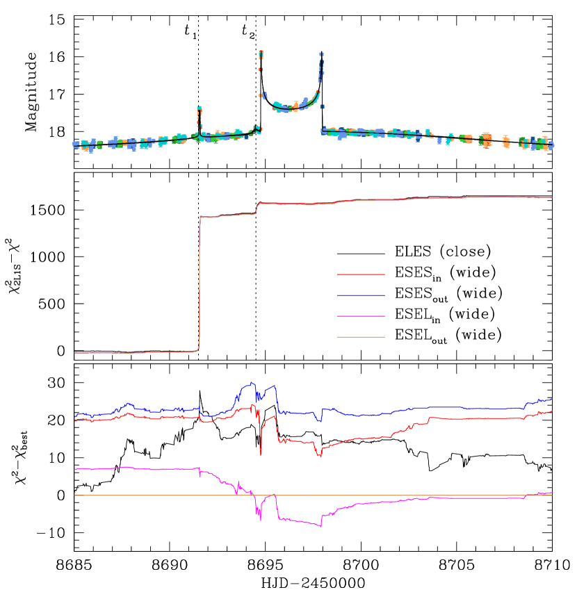
Figure 10.— Middle panel: cumulative distributions of $\Delta\chi^{2}=\chi^{2}_{\rm 2L1S}-\chi^{2}$ for the five degenerate models from the base 2L1S model. The light curve in the top panel is inserted to show where the fit improves. The two dotted lines indicate the times of the major ($t_{1}$) and minor ($t_{2}$) anomalies. Bottom panel: cumulative distributions of the $\chi^{2}$ differences from the best-fit solution, i.e., $\Delta\chi^{2}=\chi^{2}-\chi^{2}_{\rm ESEL_{out}}$.

6. Einstein radius

Measurement of $\theta_{\rm E}$ requires one to estimate the source radius, i.e., $\theta_{\rm E}=\theta_{*}/\rho$. We derive $\theta_{*}$ from the source color and brightness measured by regressing the observed $V$ and $I$ photometric data with the variation of the event magnification. We then estimate de-reddened values, $(V-I,I)_{0}$, by calibrating the instrumental values, $(V-I,I)$. This calibration is done utilizing the Yoo et al. (2004) method, in which the reference position in the color-magnitude diagram (CMD) for the calibration is the centroid of red giant clump (RGC) with $(V-I,I)_{{\rm RGC},0}=(1.060,14.347)$ known by Bensby et al. (2013) and Nataf et al. (2013).

In Figure 11, we mark the source (black dot) in the CMD. We also mark the RGC centroid and blend. We will discuss in more detail about the nature of the blend in Section 7. We note that the source position is determined using the ELES solution for the reason to be discussed in Sect 7. The source positions based on the other solutions are marked by grey-tone points. The measured color and magnitude are $(V-I,I)=(1.703\pm 0.024,20.963\pm 0.003)$ for the source and $(V-I,I)_{\rm RGC}=(1.978,15.688)$ for the RGC centroid. With the measured offsets in the source color, $\Delta(V-I)$, and magnitude, $\Delta I$, from the RGC centroid, the color and magnitude are calibrated as

 

$${(V-I,I)_{0}}$$

  (1)

The measured values points out that the source is a main sequence of a late G type. We note that the source is well below the brightness limit of Gaia observation.

In order to estimate the source radius, we convert $V-I$ into $V-K$, and interpolate $\theta_{*}$ from the $(V-K)$–$\theta_{*}$ relation. Here we use the Bessell & Brett (1988) relation for the color conversion, and the Kervella et al. (2004) relation to derive $\theta_{*}$. The source is estimated to have a radius of

$$\theta_{*}=0.41\pm 0.03~{}\mu{\rm as}.$$ (2)

For $\theta_{*}$ estimation, the source is assumed to lie at $D_{\rm S}=d_{\rm GC}/[\cos l+\sin l(\cos\phi/\sin\phi)]\sim 7.85$ kpc, where we adopt a Galactocentric distance of $d_{\rm GC}=8.16$ kpc and a bulge bar orientation angle of $\phi=40^{\circ}$. The error of the $\theta_{*}$ measurement is estimated based on the error of the measured source color and adding 7% error in quadrature to account for combined uncertainty resulting from the RGC centroiding and the color-$\theta_{*}$ conversion. We note that the source companion contributes little flux, $q_{F}/(1+q_{F})\sim 4\%$, to the combined source flux, and thus its effect on the estimated $\theta_{*}$ is minimal. Together with $\rho$ and $t_{\rm E}$, the measured $\theta_{*}$ yields the Einstein radius and the relative lens-source proper motion of

$$\theta_{\rm E}={\theta*\over\rho}=0.91\pm 0.07~{}{\rm mas},$$ (3)

and

$$\mu={\theta_{\rm E}\over t_{\rm E}}=7.59\pm 0.59~{}{\rm mas}~{}{\rm yr}^{-1},$$ (4)

respectively. The estimated value of $\theta_{\rm E}$ is substantially bigger than typical value of $\sim 0.5$ mas for events with low-mass stellar lenses lying about halfway between Earth and the bulge. This suggests that the lens lies at a close distance.

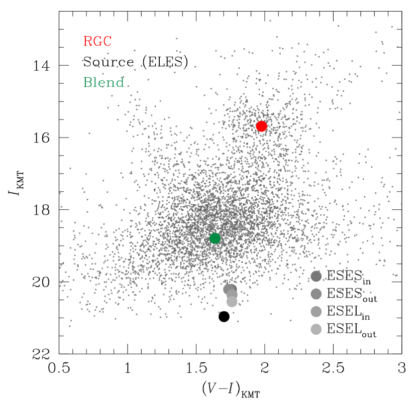
Figure 11.— Source, RGC centroid, and blend positions in the CMD. The source position is determined based on the ELES solution and those based on the other solutions are marked by grey-tone points.

7. Resolving Degeneracy

We check whether the degeneracies among the solutions can be resolved. For this, we compare the flux ratio between $S_{1}$ and $S_{2}$ measured from modeling, $q_{F,{\rm model}}=F_{S,2}/F_{S,1}$, with the flux ratio predicted from the radius ratio $\rho_{2}/\rho_{1}$, $q_{F,{\rm pred}}$. The radius ratio $\rho_{2}/\rho_{1}$ is measurable for the solutions in which the major anomaly is explained by the caustic crossing of $S_{2}$, i.e., ESXX models. We note that the major anomaly for the ELES model is explained by the caustic crossing of $S_{1}$ instead of $S_{2}$, and thus this method cannot be applied. In order to estimate $q_{F,{\rm pred}}$ from the $\rho_{2}/\rho_{1}$ ratio, we first estimate the physical radius of $S_{2}$ by

$$R_{*,S_{2}}=\left({\rho_{2}\over\rho_{1}}\right)R_{*,S_{1}}.$$ (5)

The ESXX solutions result in similar values of the color and brightness, as shown in Figure 11, and thus we use a common physical source radius of $R_{*,S_{1}}\sim 0.85~{}R_{\odot}$, which is deduced from $(V-I)_{0}$ and $I_{0}$. We then estimate the absolute $I$-band magnitudes of the source stars, $M_{I,1}$ and $M_{I,2}$, corresponding to $R_{*,S_{1}}$ and $R_{*,S_{2}}$ from the tables of Pecaut et al. (2012) and Pecaut & Mamajek (2013), and compute the flux ratio between $S_{1}$ and $S_{2}$ as

$$q_{F,{\rm pred}}=10^{-0.4(M_{I,2}-M_{I,1})}.$$ (6)

We note that a similar method could, in principle, be applied to the flux ratio $q_{F,3}=F_{S,3}/F_{S,1}$ for the models with three source stars, i.e., ESES solutions. However, the normalized radius of the tertiary source, $\rho_{3}$, is measured for none of the ESES model, and thus the method cannot be implemented.

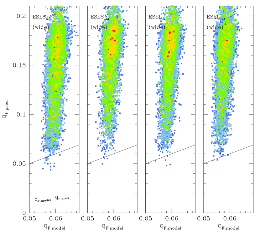
Figure 12.— Plot of $q_{F,{\rm pred}}$ versus $q_{F,{\rm model}}$ for the models explaining the major anomaly by introducing an extra source. Color codings represent points with $\leq 1\sigma$ (red), $\leq 2\sigma$ (yellow), $\leq 3\sigma$ (green), $\leq 4\sigma$ (cyan), and $\leq 5\sigma$ (blue). The oblique solid line in each panel represents the positions at which $q_{F,{\rm pred}}=q_{F,{\rm model}}$.

Figure 12 shows the scatter plot of points in the MCMC chains on the $q_{F,{\rm model}}$–$q_{F,{\rm pred}}$ parameter plane for the four tested ESXX models. In the plot, the color coding represents points with $\leq 1\sigma$ (red), $\leq 2\sigma$ (yellow), $\leq 3\sigma$ (green), $\leq 4\sigma$ (cyan), and $\leq 5\sigma$ (blue). The oblique solid line in each panel represents the positions at which $q_{F,{\rm pred}}=q_{F,{\rm model}}$. The plots show that the hypothesis of the second source’s caustic crossing for the origin of the major anomaly is rejected at more than $3\sigma$ level, suggesting that the ESXX models are unlikely to be correct interpretations of the event. With these solutions rejected, the ELES solutions remain as the only viable interpretation of the event.

8. Physical lens parameters

Recognizing that only the ELES models provide plausible interpretations of the observed lensing data, the lens parameters of the lens mass, $M$, and distance, $D_{\rm L}$, are estimated based on the observables of the ELES solutions. In order to unambiguously determine these parameters, one should measure both $\theta_{\rm E}$ and $\pi_{\rm E}$, where $\pi_{\rm E}$ represents the microlens parallax (hereafter parallax), i.e.,

$$M={\theta_{\rm E}\over\kappa\pi_{\rm E}};\qquad D_{\rm L}={{\rm au}\over\pi_{\rm E}\theta_{\rm E}+\pi_{\rm S}}.$$ (7)

Here $\kappa=4G/(c^{2}{\rm au})$, $D_{\rm S}$ is the source distance, and $\pi_{\rm S}={\rm au}/D_{\rm S}$. The Einstein radius is firmly measured, i.e., Equation (3). An additional modeling conducted considering the parallax effect indicates that secure determinations of the parallax parameters are difficult. Although $\pi_{\rm E}$ is not measured, the lensing observables of $t_{\rm E}$ and $\theta_{\rm E}$ are related as

$$t_{\rm E}={\theta_{\rm E}\over\mu};\qquad\theta_{\rm E}=(\kappa M\pi_{\rm rel})^{1/2},$$ (8)

where $\pi_{\rm rel}={\rm au}(D_{\rm L}^{-1}-D_{\rm S}^{-1})$. Then, the lens parameters can be estimated by conducting a Bayesian analysis with the prior Galactic model, defining the mass function, physical, and dynamical distributions.

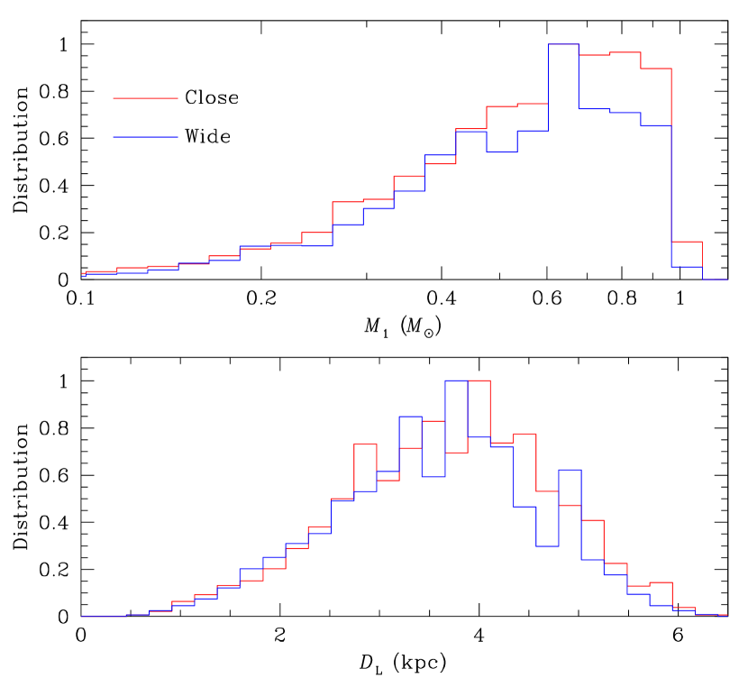
Figure 13.— Bayesian posterior distributions of $M_{1}$ and $D_{\rm L}$. The red and blue curves represent the distributions corresponding to the close and wide models, respectively.

The Bayesian analysis is carried out in two steps. The first step is producing events from a Monte Carlo simulation using a Galactic model. The models used for the analysis include Han & Gould (2003), Han & Gould (1995), Zhang et al. (2020) models for the physical, dynamical distributions, and mass function, respectively. See section 5 of Han et al. (2020b) for more details about the models. In the second step, the posterior distributions of $M$ and $D_{\rm L}$ are constructed for the events with observables, i.e., $t_{\rm E}$ and $\theta_{\rm E}$, in the 1$\sigma$ ranges of the estimated observables among the events produced from the simulation.

The posterior distributions $M_{1}$ and $D_{\rm L}$ derived from the ELES solutions are shown in Figure 13, where the red curve is the distribution resulting from the close solution, while the blue curve is the one from the wide solution. In Table 7, we summarize the estimated parameters of $M_{1}$, $M_{2}$, $M_{3}$, $D_{\rm L}$, $d_{\perp,2}$, and $d_{\perp,3}$, where the last two quantities are the separations of $M_{2}$ and $M_{3}$ from $M_{1}$. The listed values are the medians of the posterior distributions with errors determined as 16% and 84% ranges. According to the estimated parameters from the close model, the lens is a planetary system, in which a giant planet with a mass

$$M_{p}=2.56^{+1.13}_{-1.16}~{}M_{\rm J}$$ (9)

belongs to a stellar binary composed of K and M dwarfs with masses

$$M_{1}=0.61^{+0.27}_{-0.28}~{}M_{\odot},$$ (10)

and

$$M_{2}=0.15^{+0.07}_{-0.07}~{}M_{\odot},$$ (11)

respectively. As predicted by the large $\theta_{\rm E}$, the lens is located at a close distance of

$$D_{\rm L}=3.86^{+1.00}_{-1.12}~{}{\rm kpc},$$ (12)

suggesting that it is a disk object. The lens parameters derived from the wide model are also listed in Table 7. According to the ELES models, the lens is the seventh microlensing system with a planet in a stellar binary, followed by OGLE-2006-BLG-284L (Bennett et al., 2020), OGLE-2007-BLG-349L (Bennett et al., 2016), OGLE-2008-BLG-092L (Poleski et al., 2014), OGLE-2013-BLG-0341L (Gould et al., 2014), OGLE-2016-BLG-0613L (Han et al., 2017), and OGLE-2018-BLG-1700L (Han et al., 2020a).

Table 7Physical lens parameters

Parameter	Close	Wide
$M_{1}$ ($M_{\odot}$)	$0.61^{+0.27}_{-0.28}$	$0.59^{+0.26}_{-0.26}$
$M_{2}$ ($M_{\odot}$)	$0.15^{+0.07}_{-0.07}$	$0.27^{+0.12}_{-0.12}$
$M_{3}$ ($M_{\rm J}$)	$2.56^{+1.13}_{-1.16}$	$1.43^{+0.62}_{-0.62}$
$D_{\rm L}$ (kpc)	$3.86^{+1.00}_{-1.12}$	$3.77^{+0.98}_{-1.13}$
$d_{\perp,2}$ (au)	$1.73^{+0.43}_{-0.48}$	$7.82^{+2.04}_{-2.35}$
$d_{\perp,3}$ (au)	$3.32^{+0.82}_{-0.92}$	$2.80^{+0.73}_{-0.84}$

The estimated physical lens parameters suggest the possibility that the majority of the blended light comes from the lens. In Figure 11, We mark the blend, with $(V-I,I)_{b}\sim(1.6,18.8)$, in the CMD. According to the estimated $M$ and $D_{\rm L}$, the predicted brightness and color of the primary lens, which explains most of the flux from the lens, are in the ranges of

$$18.3\lesssim I_{\rm L}\lesssim 22.3$$ (13)

and

$$1.3\lesssim(V-I)_{\rm L}\lesssim 2.9.$$ (14)

Here we compute the lens brightness and color by $I_{\rm L}=M_{I}+5\log D_{\rm L}-5+A_{I}$ and $(V-I)_{\rm L}=(V-I)_{0}+E(V-I)$, where $M_{I}$ and $(V-I)_{0}$ are the absolute $I$-band magnitude and intrinsic color corresponding to $M_{1}$, and we assume $A_{I}\sim 0.5$ and $E(V-I)\sim 0.4$ by adopting the half of the values to the source considering $D_{\rm L}$. Then, the color and brightness of the blend are within the predicted ranges of the lens.

We further check this hypothesis by measuring the offset between the centroid of the apparent source image at the baseline and the source position in the difference image during the lensing magnification. We measure

$$(\Delta x,\Delta y)=(0.21\pm 0.10,0.19\pm 0.18)~{}{\rm arcsec}.$$ (15)

Considering that the measured offset is within $\sim 2\sigma$ of the measurement error, the hypothesis cannot be ruled out. Therefore, an important portion of the blended light may come from the lens, but this can only be established using high-resolution images that can be obtained from future observations with the use of adaptive optics (AO) instrument mounted on 8m-class telescopes or space-based telescopes.

9. Summary

We present the result from the investigation of KMT-2019-BLG-1715. The event light curve displayed two anomalies from a typical caustic-crossing binary-lensing light curve. We identified five pairs of solutions, in which the anomalies were explained with the inclusion of an extra lens or source component in addition to the base binary-lens model. We presented detailed analysis for the individual solutions, and trace the origins of degeneracies. To resolve the degeneracies, we compare the measured $S_{1}/S_{2}$ flux ratio with the ratio deduced from the ratio of the source radii. Applying this method left only a single pair of viable solutions, in which the anomaly with a large deviation was produced by a third body of the lens, and the anomaly with a small deviation was generated by a second source. A Bayesian analysis indicated that the lens comprised a $\sim 2.6~{}M_{\rm J}$ planet and binary stars with K and M spectral types lying in the disk. We pointed out that the lens might be the blend, and this hypothesis could be confirmed from future high-resolution followup observations.

References

- Alard & Lupton (1998) Alard, C., & Lupton, R. H. 1998, ApJ, 503, 325
- Albrow (2017) Albrow, M. 2017, MichaelDAlbrow/pyDIA: Initial Release on Github,Version v1.0.0, Zenodo, doi:10.5281/zenodo.268049
- Albrow et al. (2001) Albrow, M. D., An, J., Beaulieu, J.-P., et al. 2001, ApJ, 549, 759
- Alcock et al (1997) Alcock, C., Allsman, R. A., Alves, D., et al. 1997, ApJ, 479, 119
- An & Han (2002) An, J. H., & Han, C. 2002, ApJ, 573, 351
- Bennett (2010) Bennett, D. P. 2010, ApJ, 716, 1408
- Bennett et al. (2016) Bennett, D. P., Rhie, S. H., Udalski, A., et al. 2016, AJ, 152, 125
- Bennett et al. (2020) Bennett, D. P., Udalski, A., Bond, I. A., et al. 2020, AJ, 160, 72
- Bensby et al. (2013) Bensby, T., Yee, J. C., Feltzing, S., et al. 2013, A&A, 549, 147
- Bessell & Brett (1988) Bessell, M. S., & Brett, J. M. 1988, PASP, 100, 1134
- Bond et al. (2001) Bond, I. A., Abe, F., Dodd, R. J., et al. 2001, MNRAS, 327, 868
- Bond et al. (2002) Bond, I. A., Rattenbury, N. J., Skuljan, J., et al. 2002, MNRAS, 333, 71
- Bozza (1999) Bozza, V. 1999, A&A, 348, 311
- Bozza et al. (2018) Bozza, V., Bachelet, E., Bartolić, F., Heintz, T. M., Hoag, A. R., & Hundertmark, M. 2018, MNRAS, 479, 5157
- Bozza et al. (2012) Bozza, V., Dominik, M., Rattenbury, N. J., et al. 2012, MNRAS, 424, 902
- Daněk & Heyrovský (2015) Daněk, K., & Heyrovský, D. 2015, ApJ, 806, 99
- Daněk & Heyrovský (2019) Daněk, K., & Heyrovský, D. 2019, ApJ, 880, 72
- Di Stefano & Mao (1996) Di Stefano, R., & Mao, S. 1996, ApJ, 457, 93
- Dominik (1999) Dominik, M. 1999, A&A, 349, 108
- Dong et al. (2009) Dong, S., Bond, I. A., Gould, A., et al. 2009, ApJ, 698, 1826
- Gaudi (1998) Gaudi, B. S. 1998, ApJ, 506, 533
- Gaudi et al. (1998) Gaudi, B. S., Naber, R. M., & Sackett, P. D. 1998, ApJ, 502, L33
- Gaudi & Gould (1997) Gaudi, B. S., & Gould A. 1997, ApJ, 486, 85
- Gaudi & Han (2004) Gaudi, B. S., & Han, C. 2004, ApJ, 611, 528
- Gould (1992) Gould, A. 1992, ApJ, 392, 442
- Gould & Gaucherel (1997) Gould, A., & Gaucherel, C. 1997, ApJ, 477, 580
- Gould et al. (2014) Gould, A., Udalski, A., Shin, I.-G., et al. 2014, Science, 345, 46
- Griest & Safizadeh (1998) Griest, K., & Safizadeh, N. 1998, ApJ, 500, 37
- Han et al. (2001) Han, C., Chang, H.-Y., An, J. H., & Chang, K. 2001, MNRAS, 328, 986
- Han & Gould (1995) Han, C., & Gould, A. 1995, ApJ, 447, 53
- Han & Gould (2003) Han, C., & Gould, A. 2003, ApJ, 592, 172
- Han et al. (2021) Han, C., Lee, C.-U., Ryu, Y.-H., et al. 2021, A&A, in press [arXiv:2102.01806]
- Han et al. (2020a) Han, C., Lee, C.-U., Udalski, A., et al. 2020a, AJ, 159, 48
- Han et al. (2020b) Han, C., Shin, I.-G., Jung, Y. K., et al. 2020b, A&A, 641, A105
- Han et al. (2017) Han, C., Udalski, A., Gould, A., et al. 2017, AJ, 154, 223
- Hwang et al. (2013) Hwang, K. -H., Choi, J. -Y., Bond, I. A., et al. 2013 ApJ, 778, 55
- Hwang et al. (2018) Hwang, K.-H., Udalski, A., Bond, I. A., et al. 2018, AJ, 155, 259
- Kervella et al. (2004) Kervella, P., Thévenin, F., Di Folco, E., & Ségransan, D. 2004, A&A, 426, 29
- Kim et al. (2016) Kim, S.-L., Lee, C.-U., Park, B.-G., et al. 2016, JKAS, 49, 37
- Mao & Paczyński (1991) Mao, S., & Paczyński, B. 1991, ApJ, 374, 37
- Nataf et al. (2013) Nataf, D. M., Gould, A., Fouqué, P., et al. 2013, ApJ, 769, 88
- Pecaut & Mamajek (2013) Pecaut, M. J. & Mamajek, E. E. 2013, ApJS, 208, 9
- Pecaut et al. (2012) Pecaut, M. J., Mamajek, E. E., & Bubar, E. J. 2012, ApJ, 746, 154
- Poleski et al. (2014) Poleski, R., Skowron, J., Udalski, A., et al. 2014, ApJ, 795, 42
- Ryu et al. (2010) Ryu, Y. -H., Han, C., Hwang, K.-H., et al. 2010, ApJ, 723, 81
- Udalski (2003) Udalski, A. 2003, Acta Astron., 53, 291
- Udalski et al. (2015) Udalski, A., Szymański, M. K., & Szymański, G. 2015, Acta Astron., 65, 1
- Udalski et al. (1994a) Udalski, A., Szymański, M., Kałużny, J., Kubiak, M., Mateo, M., & Krzemiński, W. 1994, Acta Astron. 44, 1
- Udalski et al. (1994b) Udalski, A., Szymański, M., Mao, S., Di Stefano, R., Kałużny, J., Kubiak, M., Mateo, M., & Krzemiński, W. 1994, ApJ, 436, L103
- Woźniak (2000) Woźniak, P. R. 2000, Acta Astron., 50, 42
- Yee et al. (2012) Yee, J. C., Shvartzvald, Y., Gal-Yam, A., et al. 2012, ApJ, 755, 102
- Yoo et al. (2004) Yoo, J., DePoy, D. L., Gal-Yam, A., et al. 2004, ApJ, 603, 139
- Zhang et al. (2020) Zhang, X., Zang, W., Udalski, A., et al. 2020, AJ, 159, 116