Asymptotic behaviour of a linearized water waves
system in a rectangle

Abstract

We consider the asymptotic behaviour of small-amplitude gravity water waves in a rectangular domain where the water depth is much smaller than the horizontal scale. The control acts on one lateral boundary, by imposing the horizontal acceleration of the water along that boundary, as a scalar input function $u$. The state $z$ of the system consists of two functions: the water level $\zeta$ along the top boundary, and its time derivative $\frac{{\partial}\zeta}{{\partial}t}$. We prove that the solution of the water waves system converges to the solution of the one dimensional wave equation with Neumann boundary control, when taking the shallowness limit. Our approach is based on a special change of variables and a scattering semigroup, which provide the possiblity to apply the Trotter-Kato approximation theorem. Moreover, we use a detailed analysis of Fourier series for the dimensionless version of the partial Dirichlet to Neumann and Neumann to Neumann operators introduced in [1].

1 Introduction and main results

In this work we study the asymptotic behaviour of a system describing small-amplitude water waves in a rectangular domain, in the presence of a wave maker, where the horizontal scale $L$ is much larger than the typical water depth $h_{0}$. The construction of the water waves model begins from the so-called Zakharov-Craig-Sulem formulation (ZCS), which is a fully nonlinear and fully dispersive model in terms of the elevation of the free surface and the free surface velocity potential (see, for instance, Lannes’ book [2]). Based on some assumptions on the nonlinearity and the topography of the fluid domain, described by the shallowness parameter

$$\mu=\frac{h_{0}^{2}}{L^{2}},$$ (1.1)

there are many asymptotic models in the shallow water regime. The nonlinear shallow water equations is an approximation of ZCS where all the terms of order $O(\mu)$ are dropped, so that it is a fully nonlinear and non-dispersive model. Moreover, the Boussinesq equations is an approximation of ZCS of order $O(\mu^{2})$ with the weak nonlinearity assumption. The full justification (convergence) of the shallow water approximation of ZCS models mentioned above are provided in [2, Chapter 5 and Chapter 6] by considering the corresponding Cauchy problem in a strip domain that is unbounded in the horizontal direction. For more interesting asymptotic models, please refer to Lannes [2], [3] and also thereins.

Here, instead of considering a fluid filling an infinite strip, we consider the similar topic on the linearized water waves equation in a rectangular domain with a wave maker applied from the lateral boundary. Our aim is to describe the dynamics of this system when the shallowness parameter tends to zero. Now let us precisely state the problem.

The domain ${\Omega}$ is bounded by a top free surface $\Gamma_{s}$ and a flat bottom $\Gamma_{f}$. The other two components of the fluid domain, denoted by $\Gamma_{1}$ and $\Gamma_{2}$, are vertical walls, see Figure 1. The fluid filling the rectangular domain

$${\Omega}{\hbox{\hskip 1.0pt}}={\hbox{\hskip 1.0pt}}\left\{(x,y){\hbox{\hskip 1.0pt}}\left|{\hbox{\hskip 1.0pt}}(x,y)\in(0,\pi L)\times(-h_{0},0)\right\}\right.$$

is assumed to be homogeneous, incompressible, inviscid and irrotational. There is a wave maker that acts at the left boundary of ${\Omega}$, by imposing the acceleration of the fluid in the horizontal direction, as a scalar input signal $u$.

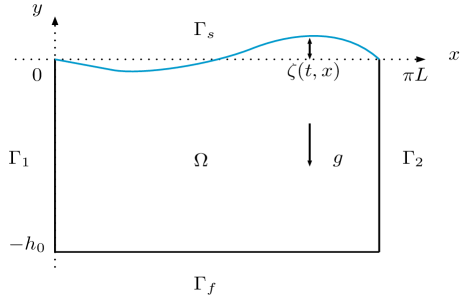
Figure 1: A rectangular domain ${\Omega}$ filled with water

We consider the water waves system in the shallow water configurations, in the sense that $\mu\ll 1$. In order to study the asymptotic behaviour of the above system, we define the following dimensionless quantities,

$$\tilde{x}=\frac{x}{L},\quad\tilde{y}=\frac{y}{h_{0}},\quad\tilde{t}=\frac{t}{L/\sqrt{gh_{0}}},\quad\tilde{\zeta}=\frac{\zeta}{a},\quad\tilde{\phi}=\frac{\phi}{aL\sqrt{g/h_{0}}},\vspace{-0.5mm}$$ (1.2)

where $a$ is the order of the surface variation, $\phi$ is the velocity potential of the fluid, $\zeta$ is the elevation of the top free surface and $g$ represents the gravity acceleration. The quantities in (1.2) marked with a tilde are their corresponding dimensionless version. With the variables $\tilde{x}$ and $\tilde{y}$, the dimensionless domain, denoted by $\tilde{\Omega}$, is

$$\tilde{\Omega}{\hbox{\hskip 1.0pt}}={\hbox{\hskip 1.0pt}}\left\{(\tilde{x},\tilde{y}){\hbox{\hskip 1.0pt}}\left|{\hbox{\hskip 1.0pt}}(\tilde{x},\tilde{y})\in(0,\pi)\times(-1,0)\right\}\right..$$ (1.3)

For the sake of simplicity, we omit the tildes in what follows and from now we always use the dimensionless quantities. Moreover, to avoid any confusion we use the notation $\zeta_{\mu}$ and $\phi_{\mu}$, instead of $\zeta$ and $\phi$, to represent the unknown functions in the dimensionless equation. The governing equations of the water waves system described above (1.2), for all $t\geqslant 0$, are

$$\left\{\begin{aligned} &\Delta_{\mu}{\hbox{\hskip 1.0pt}}\phi_{\mu}(t,x,y){\hbox{\hskip 1.0pt}}={\hbox{\hskip 1.0pt}}0\quad&\quad(\ (x,y)\in{\Omega}),\\ &\frac{{\partial}\zeta_{\mu}}{{\partial}t}(t,x){\hbox{\hskip 1.0pt}}-{\hbox{\hskip 1.0pt}}\frac{1}{\mu}{\hbox{\hskip 1.0pt}}\frac{{\partial}\phi_{\mu}}{{\partial}y}(t,x,0)=0\quad&\quad(\ x\in(0,\pi)),\\ &\frac{{\partial}\phi_{\mu}}{{\partial}t}(t,x,0)+\zeta_{\mu}(t,x){\hbox{\hskip 1.0pt}}={\hbox{\hskip 1.0pt}}0\quad&\quad(\ x\in(0,\pi)),\\ &\frac{{\partial}\phi_{\mu}}{\partial x}(t,0,y){\hbox{\hskip 1.0pt}}={\hbox{\hskip 1.0pt}}-h(y)v(t)\quad&\quad(\ y\in(-1,0)),\\ &\frac{{\partial}\phi_{\mu}}{{\partial}y}(t,x,-1)=0={\hbox{\hskip 1.0pt}}\frac{{\partial}\phi_{\mu}}{{\partial}x}(t,\pi,y)\quad&\quad(\ (x,y)\in{\Omega}),\end{aligned}\right.$$ (1.4)

where $v$ is the velocity produced by the wave maker. In the above equations $\Delta_{\mu}=\mu\frac{{\partial}^{2}}{{\partial}x^{2}}+\frac{{\partial}^{2}}{{\partial}y^{2}}$ is called the ”twisted” Laplace operator (see [2]), and the function $h$ represents the profile of the velocity imposed by the wave maker. The system (1.4) is actually a fully linear and fully dispersive approximation of ZCS constrained in a rectangle.

The controllability properties of the system derived by (1.4), as far as we know, are firstly studied in Russell and Reid [4] and further in Mottelet [5]. Now we recall here some recent works on the similar problem. Different with the control introduced in the system (1.4), Alazard discussed in [6] the stabilization of the nonlinear water waves system in a rectangle where the external pressure as the control signal acts on a part of the free surface, by absorbing the waves coming from the left. For the problem in a cubic domain, in an irregular domain and the case of the water waves with surface tension, please refer to Reid [7] and [8], Craig et al. [9], Alazard et al. [10] and [11]. Recently, for $u\in{L^{2}_{\rm loc}[0,\infty)}$, we established in our paper [1] the well-posedness of the system (1.4), and further showed that it can be recast as a well-posed linear control system (for this concept, please refer to [1], Weiss [12] or Tucsnak and Weiss [13]).

Observe that the free surface equations of (1.4) determine the whole system, which means that if we know $\psi_{\mu}(t,x)=\phi_{\mu}(t,x,0)$, thereby the velocity potential $\phi_{\mu}$ can be obtained by solving a boundary value problem for Laplacian. As explained in [1], with the help of the Dirichlet to Neumann and the Neumann to Neumann operators, the system (1.4) reduces to a second-order evolution equation in terms of $\zeta_{\mu}$. We thus propose the corresponding initial data

$$\zeta_{\mu}(0,x)=\zeta_{0}(x),\quad~{}\frac{{\partial}\zeta_{\mu}}{{\partial}t}(0,x)=\zeta_{1}(x).$$ (1.5)

Therefore, we take the acceleration $u=\frac{dv}{dt}$ as the input signal. We will provide in Section 3 more details about the formulation of the governing equations (1.4).

To state our main result, we introduce the following wave equation defined on $(0,\pi)$ with Neumann boundary control, i.e. for all $t\geqslant 0$, $x\in(0,\pi)$,

$$\left\{\begin{aligned} &\frac{{\partial}^{2}\zeta}{{\partial}t^{2}}(t,x)-\frac{{\partial}^{2}{\hbox{\hskip 1.0pt}}\zeta}{{\partial}x^{2}}(t,x)=0,\\ &\frac{{\partial}{\hbox{\hskip 1.0pt}}\zeta}{{\partial}x}(t,0)=u(t),\quad\frac{{\partial}{\hbox{\hskip 1.0pt}}\zeta}{{\partial}x}(t,\pi)=0,\\ &\zeta(0,x)=\zeta_{0}(x),\quad~{}\frac{{\partial}\zeta}{{\partial}t}(0,x)=\zeta_{1}(x).\end{aligned}\right.\vspace{-1mm}$$ (1.6)

The main contribution brought in by this work is that we justify the passage to the limit from the linear water waves system (1.4) to the system (1.6) (i.e. showing that, in an appropriate sense, $\zeta_{\mu}\to\zeta$) with the same initial data $\zeta_{0}$ and $\zeta_{1}$, as the shallowness parameter $\mu$ goes to zero.

Intuitively, the rectangular domain will reduce to a one dimensional interval when the fluid domain becomes thinner and thinner in the vertical direction. From another point of view, the dispersion relation (that is the relation between $\omega$ and $\kappa$ when the solution takes the form ${\rm e}^{{\rm i}(\kappa x-\omega t)}$) of the linearized water waves is $\omega^{2}=g\kappa\tanh\kappa h_{0}$, where $\omega$ is the angular frequency, $\kappa$ is the wave number and $h_{0}$ is the typical depth of the fluid domain. For more details about this, we refer to [2, Chapter 1] and to Whitham [14, Chapter 13]). It is obvious that the dispersion relation is approximately $\omega^{2}\sim gh_{0}\kappa^{2}$ as $\kappa h_{0}\to 0$ and the phase speed $c_{0}=\sqrt{gh_{0}}$ becomes independent of $\kappa$. The dispersive effects drop out in this limit, and in one dimension, this is exactly the property of the wave equation.

In [1] we assumed that the shape function $h$ satisfies zero mean condition $\int_{-1}^{0}h(y){\hbox{\hskip 1.0pt}}{\rm d}\hbox{\hskip 0.5pt}y=0$, to ensure the conservation of the volume of the water. This condition should be removed in this paper since the system under consideration is in the shallow water regime, where the velocity of the fluid is independent of the vertical variable (see, for instance, [2] and [14]). In this case, $h$ should be a constant, which means that the velocity or the acceleration is homogeneously imposed by the wave maker from the left edge. Without loss of generality, we might as well take $h=1$.

Before stating our main results, we need some notations. Let $\mathcal{O}\subset{\mathbb{R}}^{n}$ be an open set, we use the notation $W^{k,2}(\mathcal{O})$ ($k\in{\mathbb{N}}$) for the Sobolev space formed by the distributions $f\in\mathcal{D}^{\prime}(\mathcal{O})$ having the property that $\partial^{\alpha}f\in L^{2}(\mathcal{O})$ for every multi-index $\alpha\in{\mathbb{Z}}^{n}$ with $\alpha_{j}\geqslant 0$ and $|\alpha|\leqslant k$. For $n=1$, let $W^{s,2}(\mathcal{O})$ ($s>0$) denote the fractional order Sobolev spaces obtained by interpolation via fractional powers of a positive operator (see, for instance, Lions and Magenes [15]).

Here is our main result:

Theorem 1.1.

For $u\in{L^{2}_{\rm loc}[0,\infty)}$ and for any initial data $\zeta_{0}\in W^{1,2}[0,\pi]$ and $\zeta_{1}\in L^{2}[0,\pi]$, let $\zeta_{\mu}$ be the solution of the free surface equations of (1.4) with the initial data (1.5), satisfying

$$\zeta_{\mu}\in C([0,\infty);W^{\frac{1}{2},2}[0,\pi])\cap C^{1}([0,\infty);L^{2}[0,\pi]).$$

Let $\zeta$ be the weak solution of the system (1.6) satisfying

$$\zeta\in C([0,\infty);W^{1,2}[0,\pi])\cap C^{1}([0,\infty);L^{2}[0,\pi]).$$

Then, for every $\tau>0$, we have

$$\lim_{\mu\to 0}\sup_{t\in[0,\tau]}\lVert\zeta_{\mu}-\zeta\rVert_{W^{\frac{1}{2},2}[0,\pi]}=0,$$

$$\lim_{\mu\to 0}\sup_{t\in[0,\tau]}\left\lVert\frac{{\partial}\zeta_{\mu}}{{\partial}t}-\frac{{\partial}\zeta}{{\partial}t}\right\rVert_{L^{2}[0,\pi]}=0.$$

As we expected, according to the above theorem, the elevation of the water waves system behaves like the displacement of a string in one dimension. Although we have this relationship between the water waves system and the wave equation, their controllability properties are much different. As we know, the wave equation with Neumann boundary control is exactly controllable (see [16, Part III, Chapter 8] and [17] for the sufficiently large time, and [18] for finite time interval), while the water waves system (1.4) is even not approximately controllable (see [4] and [5]).

Our approach is based on the famous Trotter-Kato approximation theorem (see, for instance, [19, Chapter 3]) and a special change of variables, as well as a detailed analysis of Fourier series. Moreover, a scattering semigroup discussed in [20] and [21] provides the possibility for us to apply the Trotter-Kato theorem to control systems.

This paper is organized as follows. We derive, in Section 2, the dimensionless Dirichlet to Neumann and Neumann to Neumann operators. Next we do some preparations in Section 3 and propose a change of variables to rewrite the control system, which allows us to apply the Trotter-Kato theorem. In Section 4 we prove two important convergence results on the resolvent of the evolution operators. Finally, in Section 5 we focus on the proof of the main results.

2 Nondimensionalization of the Dirichlet to Neumann and Neumann to Neumann maps

In this section we derive the dimensionless form of the Dirichlet to Neumann and Neumann to Neumann maps, using the dimensionless quantities introduced in (1.2). We provided in [1] a detailed construction of these two important operators allowing us to recast (1.4) as a well-posed linear control system. Following Section 4 in [1], we go back to the definition of these two operators, which is closely related to two boundary value problems for the Laplace operator in the rectangular domain ${\Omega}$. Note that, ${\Omega}$ being a rectangle, we use separation of variables and detailed analysis of Fourier series to construct the dimensionless version of all related operators.

Recalling the dimensionless quantities introduced in (1.2), it is not difficult to see that we have

$$\frac{{\partial}}{{\partial}x}=\frac{1}{L}\frac{{\partial}}{{\partial}\tilde{x}},\quad\frac{{\partial}}{{\partial}y}=\frac{1}{h_{0}}\frac{{\partial}}{{\partial}\tilde{y}},\quad\frac{{\partial}}{{\partial}t}=\frac{\sqrt{gh_{0}}}{L}\frac{{\partial}}{{\partial}\tilde{t}}.\vspace{-0.5mm}$$ (2.1)

Based on the above relations, we define the ”twisted” gradient and Laplace operators as follows ($\mu$ is given by (1.1)):

$$\nabla_{\mu}=\left(\sqrt{\mu}\frac{{\partial}}{{\partial}\tilde{x}},\ \frac{{\partial}}{{\partial}\tilde{y}}\right),\quad\Delta_{\mu}=\mu\frac{{\partial}^{2}}{{\partial}\tilde{x}^{2}}+\frac{{\partial}^{2}}{{\partial}\tilde{y}^{2}}.\vspace{-1mm}$$

Remark 2.1.

The domain in this section is the one defined in (1.3) and we still denote it by ${\Omega}$ for simplicity.

2.1 Dirichlet and Neumann maps

We present in this part the definition and some important remarks on the Dirichlet and Neumann maps in dimensionless version. Moreover, we state several results on the properties of these maps. The proofs of these results can be obtained by slight variations of the proofs of the corresponding results in [1], so that we omit the details here.

To state the definition of the Dirichlet and Neumann maps clearly, we need some notations. We set $H=L^{2}[0,\pi]$. It is known that the family $(\varphi_{k})_{k\geqslant 0}$ defined by

$$\varphi_{k}=\left\{\varphi_{0}=\frac{1}{\sqrt{\pi}},\ \sqrt{\frac{2}{\pi}}\cos(kx)\right\}\ {\hbox{$\hskip 31.29802pt\forall\;$}}x\in[0,\pi],\vspace{-1mm}$$ (2.2)

forms an orthonormal basis in $H$. The inner product in $H$ is denoted by $\langle\cdot,\cdot\rangle$ and the associated norm by $\lVert\cdot\rVert$. The Hilbert spaces $(\mathcal{H}_{\alpha})_{\alpha\geqslant 0}$ are defined by $\mathcal{H}_{0}=H$ and

$$\mathcal{H}_{\alpha}{\hbox{\hskip 1.0pt}}={\hbox{\hskip 1.0pt}}\left\{\eta\in H\ \ \left|\ \ \sum_{k\in{\mathbb{N}}}k^{2\alpha}|\langle\eta,\varphi_{k}\rangle|^{2}<\infty\right\}\right.\qquad(\alpha\geqslant 0),$$ (2.3)

with the inner products $\langle\eta,\psi\rangle_{\alpha}=\sum_{k\in{\mathbb{N}}}k^{2\alpha}\langle\eta,\varphi_{k}\rangle{\hbox{\hskip 1.0pt}}\overline{\langle\psi,\varphi_{k}\rangle}$, for all $\eta,{\hbox{\hskip 1.0pt}}\psi\in\mathcal{H}_{\alpha}$.

Proposition 2.2.

With ${\Omega}$ as in (1.3), we consider the operator $A_{1}:\mathcal{D}(A_{1})\to L^{2}({\Omega})$ defined by

$$\mathcal{D}(A_{1})=\left\{f\in W^{2,2}({\Omega})\ \ \left|\ \ \begin{matrix}f(x,0)=0,\ \frac{\partial f}{\partial y}(x,-1)=0&x\in(0,\pi)\\ \frac{\partial f}{\partial x}(0,y)=0,\ \frac{\partial f}{\partial x}(\pi,y)=0&y\in(-1,0)\end{matrix}\right.\right\},$$

$$A_{1}f=-\Delta_{\mu}f{\hbox{$\hskip 31.29802pt\forall\;$}}f\in\mathcal{D}(A_{1}).$$

Then $A_{1}$ is a strictly positive operator on $L^{2}({\Omega})$.

We know from Proposition 2.2 that the operator $A_{1}$ is invertible since it is strictly positive (see, for instance, [13, Chapter 3]). Moreover, we have $A_{1}^{-1}\in\mathcal{L}(L^{2}({\Omega}),W^{2,2}({\Omega}))$. Based on this observation, we introduce the Dirichlet map in the following proposition.

Proposition 2.3.

For every $\eta\in H$, there exists a unique function $D_{\mu}\eta\in L^{2}({\Omega})$ such that

$$\int_{\Omega}(D_{\mu}\eta)(x,y)\overline{g(x,y)}{\hbox{\hskip 1.0pt}}{\rm d}\hbox{\hskip 0.5pt}x{\hbox{\hskip 1.0pt}}{\rm d}\hbox{\hskip 0.5pt}y{\hbox{\hskip 1.0pt}}=-\int_{0}^{\pi}\eta(x)\overline{\frac{\partial(A_{1}^{-1}g)}{\partial y}(x,0)}\,{\rm d}\hbox{\hskip 0.5pt}x\ \ \forall{\hbox{\hskip 1.0pt}}g\in L^{2}({\Omega}).$$ (2.4)

Moreover, the operator $\eta\mapsto D_{\mu}\eta$ (called a partial Dirichlet map) is bounded from $H$ into $L^{2}({\Omega})$.

Remark 2.4.

For every $\eta\in H$, we have $D_{\mu}\eta\in C^{\infty}({\Omega})$ and $\Delta_{\mu}(D_{\mu}\eta)=0$. Moreover, if $D_{\mu}\eta\in C^{1}(\overline{\Omega})$, then $D_{\mu}\eta$ is the unique function in $C^{2}({\Omega})\cap C(\overline{\Omega})$ that satisfies, in the classical sense, the following dimensionless boundary value problem:

$$\left\{\begin{aligned} &\Delta_{\mu}(D_{\mu}\eta)(x,y){\hbox{\hskip 1.0pt}}={\hbox{\hskip 1.0pt}}0\quad&\quad((x,y)\in{\Omega}),\\ &(D_{\mu}\eta)(x,0){\hbox{\hskip 1.0pt}}={\hbox{\hskip 1.0pt}}\eta(x),\quad\frac{\partial(D_{\mu}\eta)}{\partial y}(x,-1){\hbox{\hskip 1.0pt}}={\hbox{\hskip 1.0pt}}0\quad&\quad\qquad(x\in(0,\pi)),\\ &\frac{\partial(D_{\mu}\eta)}{\partial x}(0,y){\hbox{\hskip 1.0pt}}={\hbox{\hskip 1.0pt}}0,\quad\frac{\partial(D_{\mu}\eta)}{\partial x}(\pi,y){\hbox{\hskip 1.0pt}}={\hbox{\hskip 1.0pt}}0\quad&\quad\qquad(y\in(-1,0)).\end{aligned}\right.$$ (2.5)

The above equations can be obtained by taking $g=\Delta_{\mu}f$ in (2.4) and cleverly choosing the test function $f\in\mathcal{D}(A_{1})$. For more details about this, please refer to [1].

Lemma 2.5.

For every $\eta\in H$, $D_{\mu}\eta$ is given, for every $x,y\in{\Omega}$, by

$$(D_{\mu}\eta)(x,y)=\sum_{k\geqslant 0}\frac{\langle\eta,\varphi_{k}\rangle}{\cosh{(\sqrt{\mu}k)}}\varphi_{k}(x)\cosh{[\sqrt{\mu}k(y+1)]},$$

where the functions $\varphi_{k}$ have been defined in (2.2). Moreover, for every $\eta\in\mathcal{H}_{3}$ we have $D_{\mu}\eta\in C^{2}(\overline{\Omega})$.

Proof.

Note that for every $\eta\in H$, we have the Fourier expansion $\eta=\sum_{k\geqslant 0}\langle\eta,\varphi_{k}\rangle\varphi_{k}$. Therefore, the formula of $D_{\mu}\eta$ directly follows from Proposition 2.3 and Remark 2.4. The remaining proof is similar to the corresponding one in [1]. ∎

We set

$$W^{1,2}_{top}({\Omega})=\{f\in\mathcal{H}^{1}({\Omega})\ \ |\ \ f(x,0)=0,\ x\in(0,\pi)\}.$$

Next we recall in what follows the definition of the Neumann map.

Proposition 2.6.

For every $v\in L^{2}[-1,0]$, there exists a unique function $N_{\mu}v\in W^{1,2}_{top}({\Omega})$ such that

$$\int_{\Omega}\nabla_{\mu}(N_{\mu}v)\cdot\overline{\nabla_{\mu}g}\,{\rm d}\hbox{\hskip 0.5pt}x\,{\rm d}\hbox{\hskip 0.5pt}y{\hbox{\hskip 1.0pt}}={\hbox{\hskip 1.0pt}}\int_{-1}^{0}v(y)\overline{g(0,y)}\,{\rm d}\hbox{\hskip 0.5pt}y{\hbox{$\hskip 31.29802pt\forall\;$}}g\in W^{1,2}_{top}({\Omega}).$$

Moreover, the operator $N_{\mu}$, called a partial Neumann map, is linear and bounded from $L^{2}[-1,0]$ to $W^{1,2}_{top}({\Omega})$.

Remark 2.7.

The above proposition can be formulated also as follows: for every $v\in L^{2}[-1,0]$, the dimensionless boundary value problem for Laplacian

$$\left\{\begin{aligned} &\Delta_{\mu}f(x,y)=0\quad&\quad((x,y)\in{\Omega}),\\ &f(x,0)=0,\quad\frac{\partial f}{\partial y}(x,-1)=0\quad&\quad(x\in(0,\pi)),\\ &\frac{\partial f}{\partial x}(0,y)=-v,\quad\frac{\partial f}{\partial x}(\pi,y)=0\quad&\quad(y\in(-1,0)),\end{aligned}\right.$$ (2.6)

admits a unique weak solution $f=N_{\mu}v\in W^{1,2}_{top}({\Omega})$. If $f\in C^{2}(\overline{\Omega})$ and $v\in C[-1,0]$, then $f=N_{\mu}v$ is the unique classical solution of (2.6).

We note that the sequence $(\psi_{k})_{k\in{\mathbb{N}}}$ defined by

$$\psi_{k}(y)=\sqrt{2}\cos{\left[(2k-1)\frac{\pi}{2}(y+1)\right]}{\hbox{$\hskip 31.29802pt\forall\;$}}k\in{\mathbb{N}},\ y\in[-1,0],$$

is an orthonormal basis in $L^{2}[-1,0]$ (see [13, Sect. 2.6]). We define the Hilbert spaces $(\mathcal{U}_{\beta})_{\beta\geqslant 0}$ by $\mathcal{U}_{0}=L^{2}[-1,0]$ and (for $\beta>0$)

$$\mathcal{U}_{\beta}{\hbox{\hskip 1.0pt}}={\hbox{\hskip 1.0pt}}\left\{v\in\mathcal{U}_{0}\ \ \left|\ \ \sum_{k\in{\mathbb{N}}}(2k-1)^{2\beta}\left|\langle v,\psi_{k}\rangle_{\mathcal{U}_{0}}\right|^{2}<\infty\right\}\right.{\hbox{\hskip 1.0pt}},$$

with the inner products given by $\langle v,w\rangle_{\mathcal{U}_{\beta}}=\sum_{k\in{\mathbb{N}}}(2k-1)^{2\beta}\langle v,\psi_{k}\rangle_{\mathcal{U}_{0}}\overline{\langle w,\psi_{k}\rangle_{\mathcal{U}_{0}}}$, for every $v,{\hbox{\hskip 1.0pt}}w\in\mathcal{U}_{\beta}$.

Lemma 2.8.

For every $v\in L^{2}[-1,0]$ and every $(x,y)\in{\Omega}$ we have

$$(N_{\mu}v)(x,y)=\sum_{k\in{\mathbb{N}}}a_{k}\cosh\left[\frac{(2k-1)}{2\sqrt{\mu}}\pi(x-\pi)\right]\cos{\left[(2k-1)\frac{\pi}{2}(y+1)\right]},$$ (2.7)

where

$$a_{k}{\hbox{\hskip 1.0pt}}={\hbox{\hskip 1.0pt}}\frac{2\sqrt{2\mu}\langle v,\psi_{k}\rangle}{(2k-1)\pi\sinh{\left[\frac{2k-1}{2\sqrt{\mu}}\pi^{2}\right]}}{\hbox{$\hskip 31.29802pt\forall\;$}}k\in{\mathbb{N}}.\vspace{-1mm}$$

Moreover, for every $v\in\mathcal{U}_{2}$ we have $N_{\mu}v\in C^{2}(\overline{{\Omega}})$.

Proof.

For every $v\in L^{2}[-1,0]$, $v=\sum_{k\in{\mathbb{N}}}\langle v,\psi_{k}\rangle\psi_{k}$. According to Proposition 2.6 and Remark 2.7, using separation of variables we immediately obtain the formula (2.7). We omit the remaining details since it is almost the same with the one in [1]. ∎

2.2 Dirichlet to Neumann and Neumann to Neumann maps

In this subsection, we derive the dimensionless version of the Dirichlet to Neumann and Neumann to Neumann operators and study their related spectral properties.

Corollary 2.9.

Let $\gamma_{1}:C^{1}(\overline{\Omega})\to C[0,\pi]$ be the partial Neumann trace operator defined by

$$(\gamma_{1}f)(x){\hbox{\hskip 1.0pt}}={\hbox{\hskip 1.0pt}}\frac{\partial f}{\partial y}(x,0){\hbox{$\hskip 31.29802pt\forall\;$}}f\in C^{1}(\overline{\Omega}),\ x\in[0,\pi].$$

Then $\tilde{A}_{\mu}$ defined by

$$\tilde{A}_{\mu}\eta{\hbox{\hskip 1.0pt}}={\hbox{\hskip 1.0pt}}\gamma_{1}D_{\mu}\eta{\hbox{$\hskip 31.29802pt\forall\;$}}\eta\in\mathcal{H}_{3},$$

called a partial Dirichlet to Neumann map, is a linear bounded map from $\mathcal{H}_{3}$ to $C[0,\pi]$.

Proposition 2.10.

The operator $\tilde{A}_{\mu}$ introduced in Corollary 2.9 has a unique continuous extension to an operator $A_{\mu}:\mathcal{H}_{1}\to H$. Then we have $A_{\mu}\varphi_{k}=\lambda_{k}\varphi_{k}$ with $(\lambda_{0}=0)$

$$\lambda_{k}{\hbox{\hskip 1.0pt}}={\hbox{\hskip 1.0pt}}\sqrt{\mu}k\tanh(\sqrt{\mu}k){\hbox{$\hskip 31.29802pt\forall\;$}}k\in{\mathbb{N}},$$

and

$$A_{\mu}\eta{\hbox{\hskip 1.0pt}}={\hbox{\hskip 1.0pt}}\sum_{k\in{\mathbb{N}}}{\lambda}_{k}\langle\eta,\varphi_{k}\rangle\varphi_{k}{\hbox{$\hskip 31.29802pt\forall\;$}}\eta\in\mathcal{H}_{1}.$$ (2.8)

Remark 2.11.

The dimensionless Dirichlet to Neumann map $A_{\mu}$ introduced in Proposition 2.10 is positive, but not strictly positive, which is the difference with the one discussed in [1]. This is induced, as explained in the introduction, by removing zero mean condition from the state space, so that the system fits in the shallow water configurations.

Corollary 2.12.

With $\gamma_{1}$ as in Corollary 2.9, define the operator $\tilde{B}_{\mu}$ by

$$\tilde{B}_{\mu}v{\hbox{\hskip 1.0pt}}={\hbox{\hskip 1.0pt}}\gamma_{1}N_{\mu}v\ {\hbox{$\hskip 31.29802pt\forall\;$}}v\in\mathcal{U}_{2},$$

called a partial Neumann to Neumann map, where $N_{\mu}$ is the Neumann map introduced in Proposition 2.6. Then $\tilde{B}_{\mu}$ is a bounded linear operator from $\mathcal{U}_{2}$ to $C[0,\pi]$.

Proposition 2.13.

The operator $\tilde{B}_{\mu}$ introduced in Corollary 2.12 can be extended in a unique manner to a linear bounded operator $B_{\mu}\in\mathcal{L}(\mathcal{U}_{0},H)$. In particular, the operator $B_{\mu}$ belongs to $\mathcal{L}({\mathbb{C}},H)$ and for every $u\in{\mathbb{C}}$

$$(B_{\mu}u)(x){\hbox{\hskip 1.0pt}}={\hbox{\hskip 1.0pt}}\sum_{k\in{\mathbb{N}}}b_{k}\cosh\left[\frac{(2k-1)}{2\sqrt{\mu}}\pi(x-\pi)\right],$$

where

$$b_{k}{\hbox{\hskip 1.0pt}}={\hbox{\hskip 1.0pt}}\frac{-4u\sqrt{\mu}}{(2k-1)\pi\sinh\left[\frac{2k-1}{2\sqrt{\mu}}\pi^{2}\right]}.$$

The proofs of Proposition 2.10 and Proposition 2.13 are completely similar with the corresponding ones for the usual Dirichlet to Neumann and Neumann to Neumann maps (with dimension) in [1]. Therefore, we omit the details here. Next we introduce a convergence property on the Neumann to Neumann map $B_{\mu}$, which plays an important role in our arguments.

Theorem 2.14.

Let $B_{0}=-\delta_{0}$, where $\delta_{0}$ is the Dirac mass concentrated at $x=0$ and let $B_{\mu}$ be the Neumann to Neumann map defined in Proposition 2.13. Then we have

$$\lim_{\mu\to 0}\left\lVert{\hbox{\hskip 1.0pt}}\frac{1}{\mu}B_{\mu}u-B_{0}u{\hbox{\hskip 1.0pt}}\right\rVert_{\left(W^{1,2}[0,\pi]\right)^{\prime}}=0{\hbox{$\hskip 31.29802pt\forall\;$}}u\in{\mathbb{C}},\vspace{-0.5mm}$$ (2.9)

where $\left(W^{1,2}[0,\pi]\right)^{\prime}$ is the dual of $W^{1,2}[0,\pi]$ with respect to the pivot space $H$.

Proof.

One readily sees that, equivalently, we need to show that for every $u\in{\mathbb{C}}$ and for every $\phi\in W^{1,2}[0,\pi]$ with $\lVert\phi\rVert_{W^{1,2}}\leqslant 1$,

$$\lim_{\mu\to 0}\sup_{\lVert\phi\rVert_{W^{1,2}}\leqslant 1}\left|\left\langle\frac{1}{\mu}B_{\mu}u{\hbox{\hskip 1.0pt}}-{\hbox{\hskip 1.0pt}}B_{0}u,\ \phi\right\rangle\right|=0.$$ (2.10)

According to Proposition 2.13, we have

$$\frac{1}{\mu}B_{\mu}u{\hbox{\hskip 1.0pt}}={\hbox{\hskip 1.0pt}}\sum_{k\in{\mathbb{N}}}c_{k}\cosh\left[\frac{(2k-1)}{2\sqrt{\mu}}\pi(x-\pi)\right],$$ (2.11)

where

$$c_{k}{\hbox{\hskip 1.0pt}}={\hbox{\hskip 1.0pt}}\frac{-4u}{\sqrt{\mu}(2k-1)\pi\sinh\left[\frac{2k-1}{2\sqrt{\mu}}\pi^{2}\right]}.$$

We denote

$$f_{k}(x){\hbox{\hskip 1.0pt}}={\hbox{\hskip 1.0pt}}\sinh\left[\frac{2k-1}{2\sqrt{\mu}}\pi x\right],\qquad$$

and obtain by using integration by parts that

$$\int_{0}^{\pi}\cosh\left[\frac{(2k-1)}{2\sqrt{\mu}}\pi(x-\pi)\right]\phi(x){\rm d}\hbox{\hskip 0.5pt}x{\hbox{\hskip 1.0pt}}=\\ {\hbox{\hskip 1.0pt}}\frac{2\sqrt{\mu}}{(2k-1)\pi}\left\{\phi(0)f_{k}(\pi)-{\hbox{\hskip 1.0pt}}\int_{0}^{\pi}\sinh\left[\frac{2k-1}{2\sqrt{\mu}}\pi(x-\pi)\right]\phi^{\prime}(x){\rm d}\hbox{\hskip 0.5pt}x\right\}.$$ (2.12)

Furthermore, note that

$$\int_{0}^{\pi}\sinh\left[\frac{2k-1}{2\sqrt{\mu}}\pi(x-\pi)\right]\phi^{\prime}(x){\hbox{\hskip 1.0pt}}{\rm d}\hbox{\hskip 0.5pt}x=\\ {\rm e}^{-\frac{2k-1}{2\sqrt{\mu}}\pi^{2}}\int_{0}^{\pi}f_{k}(x)\phi^{\prime}(x){\hbox{\hskip 1.0pt}}{\rm d}\hbox{\hskip 0.5pt}x{\hbox{\hskip 1.0pt}}-{\hbox{\hskip 1.0pt}}f_{k}(\pi)\int_{0}^{\pi}{\rm e}^{-\frac{2k-1}{2\sqrt{\mu}}\pi x}\phi^{\prime}(x){\hbox{\hskip 1.0pt}}{\rm d}\hbox{\hskip 0.5pt}x,$$

we thus have the following estimate (using (2.12))

$$\left|\left\langle\frac{1}{\mu}B_{\mu}u-B_{0}u,{\hbox{\hskip 1.0pt}}\phi\right\rangle\right|{\hbox{\hskip 1.0pt}}\leqslant{\hbox{\hskip 1.0pt}}\sum_{k\in{\mathbb{N}}}\frac{32\mu|u|}{(2k-1)^{4}\pi^{6}}{\hbox{\hskip 1.0pt}}{\rm e}^{-\frac{2k-1}{2\sqrt{\mu}}\pi^{2}}\int_{0}^{\pi}\left|f_{k}(x)\phi^{\prime}(x)\right|{\rm d}\hbox{\hskip 0.5pt}x\\ +{\hbox{\hskip 1.0pt}}\sum_{k\in{\mathbb{N}}}\frac{8|u|}{(2k-1)^{2}\pi^{2}}\int_{0}^{\pi}\left|{\rm e}^{-\frac{2k-1}{2\sqrt{\mu}}\pi x}\phi^{\prime}(x)\right|{\rm d}\hbox{\hskip 0.5pt}x.$$ (2.13)

In the above estimate, we used the fact $\sum_{k\in{\mathbb{N}}}\frac{1}{(2k-1)^{2}}=\frac{\pi^{2}}{8}$ and $\sinh x\geqslant x^{2}$ for large $x$. Note that there exists a constant $C>0$, such that ${\rm e}^{-\frac{2k-1}{2\sqrt{\mu}}\pi^{2}}f_{k}(\pi)\leqslant C$ uniformly with respect to $\mu$ and $k$, we immediately obtain that

$$\sum_{k\in{\mathbb{N}}}\frac{\mu}{(2k-1)^{4}}{\hbox{\hskip 1.0pt}}{\rm e}^{-\frac{2k-1}{2\sqrt{\mu}}\pi^{2}}\int_{0}^{\pi}\left|f_{k}(x)\phi^{\prime}(x)\right|{\rm d}\hbox{\hskip 0.5pt}x\leqslant C\sum_{k\in{\mathbb{N}}}\frac{\mu}{(2k-1)^{4}}{\hbox{\hskip 1.0pt}}\lVert\phi^{\prime}\rVert\leqslant C\mu.$$

Moreover, since $\left\lVert{\rm e}^{-\frac{2k-1}{2\sqrt{\mu}}\pi x}\right\rVert^{2}\leqslant C\frac{2\sqrt{\mu}}{(2k-1)\pi}$ we have

$$\sum_{k\in{\mathbb{N}}}\frac{1}{(2k-1)^{2}}\int_{0}^{\pi}\left|{\rm e}^{-\frac{2k-1}{2\sqrt{\mu}}\pi x}\phi^{\prime}(x)\right|{\rm d}\hbox{\hskip 0.5pt}x\leqslant C\sum_{k\in{\mathbb{N}}}\frac{\mu^{\frac{1}{4}}}{(2k-1)^{\frac{5}{2}}}{\hbox{\hskip 1.0pt}}\lVert\phi^{\prime}\rVert\leqslant C\mu^{\frac{1}{4}}.$$

Therefore, we conclude that, for every fixed $u\in{\mathbb{C}}$, the right-hand side of (2.13) can be controlled by $C\mu^{\frac{1}{4}}$, which clearly implies (2.10). ∎

3 Operator form of the governing equations

In this section, we formulate the governing equations (1.4) as a well-posed LTI (linear time-invariant) system in an appropriate Hilbert space. To this aim, we first define a scale of Hilbert spaces associated to a certain operator and then derive the dimensionless control system related to (1.4), finally formulate the control system into the one that allows us to apply the Trotter-Kato approximation theorem in Section 5.

For a self-adjoint positive operator $A:\mathcal{D}(A)\to H$ with compact resolvents, according to the classical results (see, for instance, [13, Chapter 3]), the operator $A$ is diagonalizable, also called Riesz-spectral operator in some literatures (for instance in [22]), with an orthonormal basis $(\varphi_{k})_{k\geqslant 0}$ of eigenvectors and the corresponding positive eigenvalues $(\lambda_{k})_{k\geqslant 0}$. For any $z\in H$, we denote $z_{k}=\langle z,\varphi_{k}\rangle$. Moreover, we have

$$\mathcal{D}(A){\hbox{\hskip 1.0pt}}={\hbox{\hskip 1.0pt}}\left\{z\in H\ \left|\ \ \sum_{k\geqslant 0}(1+\left|\lambda_{k}\right|^{2}){\hbox{\hskip 1.0pt}}|z_{k}|^{2}<\infty\right\}\right.,\vspace{-1mm}$$

and

$$Az{\hbox{\hskip 1.0pt}}={\hbox{\hskip 1.0pt}}\sum_{k\geqslant 0}\lambda_{k}z_{k}\varphi_{k}\qquad(z\in\mathcal{D}(A)).$$

For every $\alpha\in{\mathbb{R}}$, we introduce the scale of Hilbert spaces $H_{\alpha}$, associated to the operator $A$, which is defined by ($H_{0}=H$)

$$H_{\alpha}{\hbox{\hskip 1.0pt}}={\hbox{\hskip 1.0pt}}\left\{z\in H\ \left|\ \ \sum_{k\geqslant 0}(1+\left|\lambda_{k}\right|^{2\alpha}){\hbox{\hskip 1.0pt}}|z_{k}|^{2}<\infty\right\}\right.,\vspace{-1mm}$$

endowed with the inner product

$$\langle\eta,\upsilon\rangle_{\alpha}=\sum_{k\geqslant 0}(1+\left|\lambda_{k}\right|^{2\alpha})\eta_{k}{\hbox{\hskip 1.0pt}}\upsilon_{k}{\hbox{$\hskip 31.29802pt\forall\;$}}\eta,{\hbox{\hskip 1.0pt}}\upsilon\in H_{\alpha}.\vspace{-1mm}$$

It is obvious to see that, for every $\alpha\geqslant 0$, Hilbert space $H_{\alpha}$ is actually the domain of the operator $A^{\alpha}$ with its graph norm $\lVert\cdot\rVert_{gr}$. Furthermore, for every $\alpha\in{\mathbb{R}}$, $H_{-\alpha}$ is the dual space of $H_{\alpha}$ with respect to the pivot space $H$. We will apply, in the following part, the above definition of a scale of Hilbert spaces to different operators.

Next we formulate the equations (1.4) into a second-order evolution equation in terms of $\zeta_{\mu}$. Recalling the definition of the Dirichlet to Neumann map $A_{\mu}$ and the Neumann to Neumann map $B_{\mu}$ in Section 2, we immediately obtain from the structure of the governing equations (1.4) that

$$\frac{{\partial}\phi_{\mu}}{{\partial}y}(t,x,0)=A_{\mu}\psi_{\mu}(t,x)+B_{\mu}v(t),\vspace{-1mm}$$ (3.1)

where $t\geqslant 0$, $x\in(0,\pi)$ and $\psi_{\mu}(t,x)=\phi_{\mu}(t,x,0)$. Taking the derivative of the second equation in (1.4) with respect to time and eliminating $\psi_{\mu}(t,x)$ by using the third equation of (1.4), we get the second-order control system associated to (1.4), i.e. for all $t\geqslant 0$, $x\in(0,\pi)$,

$$\left\{\begin{aligned} &\frac{{\partial}^{2}\zeta_{\mu}}{{\partial}t^{2}}(t,x){\hbox{\hskip 1.0pt}}+{\hbox{\hskip 1.0pt}}\frac{1}{\mu}A_{\mu}\zeta_{\mu}(t,x)=\frac{1}{\mu}B_{\mu}u(t),\\ &\zeta_{\mu}(0,x)=\zeta_{0}(x),\quad\frac{{\partial}\zeta_{\mu}}{{\partial}t}(0,x)=\zeta_{1}(x),\end{aligned}\right.$$ (3.2)

where $u=\frac{dv}{dt}$ is the input signal, the operators $A_{\mu}$ and $B_{\mu}$ are defined in Proposition 2.10 and Proposition 2.13, respectively. Moreover, we introduce the operator $A_{0}:\mathcal{D}(A_{0})\to H$ as follows:

$$A_{0}=-\frac{d^{2}}{dx^{2}}\qquad\mathcal{D}(A_{0})=\left\{f\in W^{2,2}[0,\pi]{\hbox{\hskip 1.0pt}}\left|{\hbox{\hskip 1.0pt}}\frac{df}{dx}(0)=\frac{df}{dx}(\pi)=0\right.\right\}.$$ (3.3)

With the operators $B_{0}$ defined in Theorem 2.14, we consider the following evolution equation, i.e. for all $t\geqslant 0$, $x\in(0,\pi)$,

$$\left\{\begin{aligned} &\frac{{\partial}^{2}\zeta}{{\partial}t^{2}}(t,x){\hbox{\hskip 1.0pt}}+{\hbox{\hskip 1.0pt}}A_{0}\zeta(t,x)=B_{0}u(t),\\ &\zeta(0,x)=\zeta_{0}(x),\quad\frac{{\partial}\zeta}{{\partial}t}(0,x)=\zeta_{1}(x).\end{aligned}\right.\vspace{-1mm}$$ (3.4)

It is known that the operator $A_{0}$ defined in (3.3) is diagonalizable with the eigenvalues $k^{2}$ and the corresponding eigenvectors $\varphi_{k}$ are given in (2.2). For the operator $A_{0}$, we denote by $\mathbb{H}_{\alpha}$ with $\alpha\in{\mathbb{R}}$ the scale of Hilbert spaces which has been introduced at the beginning of this section. Notice that the Dirichlet to Neumann operator $A_{\mu}$ in Proposition 2.10 is also diagonalizable, so that, for $\alpha\in{\mathbb{R}}$, we denote by $H_{\mu,\alpha}$ the scale of Hilbert spaces associated to the operator $\frac{1}{\mu}A_{\mu}$. Therefore, we have $\mathbb{H}_{0}=\mathbb{H}=H=H_{\mu,0}$ and $\mathbb{H}_{-\alpha}$ (or $H_{\mu,-\alpha}$) is the dual space of $\mathbb{H}_{\alpha}$ (or $H_{\mu,\alpha}$) with respect to the pivot space $H$. It is not difficult to see that actually we have $\mathbb{H}_{\frac{1}{2}}=W^{1,2}[0,\pi]$. For more details on a scale of Hilbert space, please refer to [13, Chapter 2].

We mention that the operator $B_{\mu}$ is bounded (see Proposition 2.13), i.e. $B_{\mu}\in\mathcal{L}(\mathbb{C},H)$, and $B_{0}$ induces an admissible control operator in the first-order system associated to (3.4) with the state $\left[\begin{smallmatrix}\zeta\\ \frac{{\partial}\zeta}{{\partial}t}\end{smallmatrix}\right]$ (please refer to [13, Proposition 6.2.5]), although it is unbounded (not contained in the state space), i.e. $B_{0}\in\mathcal{L}(\mathbb{C},\mathbb{H}_{-\frac{1}{2}})$. Based on the above analysis, the system (3.4) is well-defined.

Remark 3.1.

According to Proposition 2.10, the eigenvalues of $\frac{1}{\mu}A_{\mu}$ are $\frac{k\tanh(\sqrt{\mu}k)}{\sqrt{\mu}}$, which is equivalent to $k$ for fixed $\mu\in(0,1)$. Therefore, for every $\alpha\geqslant 0$, Hilbert space $H_{\mu,\alpha}$ is actually equivalent to $\mathcal{H}_{\alpha}$ introduced in (2.3). Moreover, according to interpolation theory (see, for instance, [15], [16, Part II] and [23]), for $\alpha\in(0,1)$, the scale of Hilbert space $\mathcal{H}_{\alpha}$ is exactly the classical Sobolev space $W^{\alpha,2}[0,\pi]$.

Remark 3.2.

The initial boundary value problem (1.6) is a well-posed boundary control system (for this concept, see for instance [13, Chapter 10]), which is equivalent to (3.4) in weak sense, that is, for every $u\in{L^{2}_{\rm loc}[0,\infty)}$, for every $\zeta_{0}\in\mathbb{H}_{\frac{1}{2}}$ and $\zeta_{1}\in\mathbb{H}$, there exists a unique function

$$\zeta\in C([0,\infty);\mathbb{H}_{\frac{1}{2}})\cap C^{1}([0,\infty);\mathbb{H}),\vspace{-0.5mm}$$

such that $\zeta(0,x)=\zeta_{0}$ and it satisfies, for every $t\geqslant 0$ and every $\psi\in\mathbb{H}_{\frac{1}{2}}$,

$$\int_{0}^{\pi}\frac{{\partial}\zeta}{{\partial}t}(t,x)\overline{\psi(x)}{\hbox{\hskip 1.0pt}}{\rm d}\hbox{\hskip 0.5pt}x-\int_{0}^{\pi}\zeta_{1}(x)\overline{\psi(x)}{\hbox{\hskip 1.0pt}}{\rm d}\hbox{\hskip 0.5pt}x\\ {\hbox{\hskip 1.0pt}}={\hbox{\hskip 1.0pt}}-\int_{0}^{t}\int_{0}^{\pi}\frac{{\partial}\zeta}{{\partial}x}(\sigma,x)\overline{\frac{d\psi}{dx}(x)}{\hbox{\hskip 1.0pt}}{\rm d}\hbox{\hskip 0.5pt}x\,{\rm d}\hbox{\hskip 0.5pt}\sigma-\int_{0}^{t}u(\sigma)\overline{\psi(0)}{\hbox{\hskip 1.0pt}}{\rm d}\hbox{\hskip 0.5pt}\sigma.$$

In what follows, we are ready to study the asymptotic behaviour of the system (3.2) when $\mu$ goes to zero. We shall consider the relationship between the solutions of (3.2) and (3.4). Normally, the state of the control system is taken as $\left[\begin{smallmatrix}\zeta\\ \frac{{\partial}\zeta}{{\partial}t}\end{smallmatrix}\right]$, but the main problem lies in the difference of the energy space of (3.2) and (3.4), one is $H_{\mu,\frac{1}{2}}\times H$ and the other is $\mathbb{H}_{\frac{1}{2}}\times\mathbb{H}$. It means that we cannot apply the Trotter-Kato theorem directly. According to the classical semigroup theory (see, for instance, [13] and [22]), for $\zeta_{0}\in\mathbb{H}_{\frac{1}{2}}$ and $\zeta_{1}\in\mathbb{H}$, (3.2) and (3.4) admit a unique solution $\zeta_{\mu}$ and $\zeta$, respectively, which satisfy

$$\zeta_{\mu}\in C([0,\infty);H_{\mu,\frac{1}{2}})\cap C^{1}([0,\infty);H),$$

and

$$\zeta\in C([0,\infty);\mathbb{H}_{\frac{1}{2}})\cap C^{1}([0,\infty);\mathbb{H}).$$

We thus consider the following change of variables,

$$\alpha_{\mu}:=\frac{{\partial}\zeta_{\mu}}{{\partial}t},\qquad\beta_{\mu}:=\left(\frac{1}{\mu}A_{\mu}\right)^{1/2}\zeta_{\mu},\vspace{-1mm}$$ (3.5)

and

$$\alpha:=\frac{{\partial}\zeta}{{\partial}t},\qquad\beta:=A_{0}^{1/2}\zeta,$$ (3.6)

where $A_{0}$ and $A_{\mu}$ are introduced in (3.3) and Proposition 2.10, respectively. In this way, we have $\alpha_{\mu},{\hbox{\hskip 1.0pt}}\beta_{\mu}\in C([0,\infty);H)$ and $\alpha,{\hbox{\hskip 1.0pt}}\beta\in C([0,\infty);\mathbb{H})$. Setting

$$w_{\mu}(t)=\left[\begin{matrix}\alpha_{\mu}(t,\cdot)\\ \beta_{\mu}(t,\cdot)\end{matrix}\right]\quad\text{and}\quad w(t)=\left[\begin{matrix}\alpha(t,\cdot)\\ \beta(t,\cdot)\end{matrix}\right],$$

we obtain from (3.2) and (3.4) that

$$\left\{\begin{aligned} &\frac{dw_{\mu}}{dt}(t)=\mathscr{A}_{\mu}w_{\mu}(t)+\mathscr{B}_{\mu}u(t),\\ &w_{\mu}(0)=w_{\mu,0},\end{aligned}\right.$$ (3.7)

and

$$\left\{\begin{aligned} &\frac{dw}{dt}(t)=\mathscr{A}_{0}w(t)+\mathscr{B}_{0}u(t),\\ &w(0)=w_{0},\end{aligned}\right.$$ (3.8)

where

$$\mathscr{A}_{\mu}{\hbox{\hskip 1.0pt}}={\hbox{\hskip 1.0pt}}\left[\begin{matrix}0&-\left(\frac{1}{\mu}A_{\mu}\right)^{1/2}\\ \left(\frac{1}{\mu}A_{\mu}\right)^{1/2}&0\end{matrix}\right],\qquad\mathscr{A}_{0}{\hbox{\hskip 1.0pt}}={\hbox{\hskip 1.0pt}}\left[\begin{matrix}0&-A_{0}^{1/2}\\ A_{0}^{1/2}&0\end{matrix}\right],$$ (3.9)

$$\mathscr{B}_{\mu}=\left[\begin{matrix}\frac{1}{\mu}B_{\mu}\\ 0\end{matrix}\right],\qquad\mathscr{B}_{0}=\left[\begin{matrix}B_{0}\\ 0\end{matrix}\right],$$ (3.10)

and

$$w_{\mu,0}=\left[\begin{matrix}\zeta_{1}\\ \left(\frac{1}{\mu}A_{\mu}\right)^{1/2}\zeta_{0}\end{matrix}\right],\qquad w_{0}=\left[\begin{matrix}\zeta_{1}\\ A_{0}^{1/2}\zeta_{0}\end{matrix}\right].$$ (3.11)

Let $X=H\times H$, then the operator $\mathscr{A}_{\mu}:\mathcal{D}(\mathscr{A}_{\mu})\to X$ with $\mathcal{D}(\mathscr{A}_{\mu})=H_{\mu,\frac{1}{2}}\times H_{\mu,\frac{1}{2}}$ and $\mathscr{A}_{0}:\mathcal{D}(\mathscr{A}_{0})\to X$ with $\mathcal{D}(\mathscr{A}_{0})=\mathbb{H}_{\frac{1}{2}}\times\mathbb{H}_{\frac{1}{2}}$. Furthermore, it is not difficult to see that $\mathscr{B}_{\mu}\in\mathcal{L}({\mathbb{C}},X)$ and $\mathscr{B}_{0}\in\mathcal{L}({\mathbb{C}},\mathbb{H}_{-\frac{1}{2}}\times\mathbb{H}_{-\frac{1}{2}})$. With the help of the new variables defined in (3.5) and (3.6), the control systems we are now focusing on are (3.7) and (3.8), which possess the same state space $X$ and provide the possibility to apply the Trotter-Kato theorem.

Based on the structure of the operators $\mathscr{A}_{\mu}$ and $\mathscr{A}_{0}$, we introduce the following lemma, which is probably known in the semigroup community. However, for the sake of completeness (and with no claim of originality) we give here its precise statement and a short proof. For simplicity, we denote by $R(\lambda:A)=(\lambda I-A)^{-1}$ the resolvent of $A$ with $\lambda\in\rho(A)$ (resolvent set of $A$).

Lemma 3.3.

Let the operator $A:\mathcal{D}(A)\to H$ be positive (i.e. $A\geqslant 0$) with compact resolvents. Then the operator $\mathscr{A}:\mathcal{D}(\mathscr{A})\to X$ defined by

$$\mathcal{D}(\mathscr{A})=\mathcal{D}\left(A^{1/2}\right)\times\mathcal{D}\left(A^{1/2}\right),$$

$$\mathscr{A}\left[\begin{matrix}\varphi\\ \psi\end{matrix}\right]{\hbox{\hskip 1.0pt}}={\hbox{\hskip 1.0pt}}\left[\begin{matrix}-A^{1/2}\psi\\ A^{1/2}\varphi\end{matrix}\right],{\hbox{$\hskip 31.29802pt\forall\;$}}\left[\begin{matrix}\varphi\\ \psi\end{matrix}\right]\in\mathcal{D}(\mathscr{A}),$$

generates a unitary group on $X$.

Proof.

The operator $\mathscr{A}$ is obviously skew-symmetric since $\operatorname{Re}\langle\mathscr{A}w,w\rangle_{X}=0$ for all $w=\left[\begin{smallmatrix}w_{1}\\ w_{2}\end{smallmatrix}\right]\in\mathcal{D}(\mathscr{A})$. Note that, for every $\left[\begin{smallmatrix}f\\ g\end{smallmatrix}\right]\in X$, there exists $\varphi$ and $\psi$ defined by

$$\varphi=-R(-1:A)(f+A^{1/2}g),\qquad\psi=R(-1:A)(-g+A^{1/2}f),$$

satisfy $\varphi,{\hbox{\hskip 1.0pt}}\psi\in\mathcal{D}(A^{1/2})$ and

$$\left(I+\mathscr{A}\right)\left[\begin{matrix}\varphi\\ \psi\end{matrix}\right]=\left[\begin{matrix}f\\ g\end{matrix}\right].$$ (3.12)

Indeed, note that since $A$ is positive, then $\sigma(A)\subset[0,\infty)$, which implies $-1\in\rho(A)$, so that the operator $I+A$ is invertible. Next we show that $\varphi,{\hbox{\hskip 1.0pt}}\psi\in\mathcal{D}(A^{1/2})$. The positive operator $A^{1/2}:H_{\frac{1}{2}}\to H$ has a unique extension (still denoted by $A^{1/2}$) such that $A^{1/2}\in\mathcal{L}(H,H_{-\frac{1}{2}})$, where the Hilbert spaces $H_{s}$ $(s\in{\mathbb{R}})$ is the scale of Hilbert space associated to the operator $A$. Moreover, $A:H_{1}\to H$ also has a unique extension such that $A\in\mathcal{L}(H_{\frac{1}{2}},H_{-\frac{1}{2}})$, which implies that $R(-1,A)\in\mathcal{L}(H_{-\frac{1}{2}},H_{\frac{1}{2}})$. Thus, for every $g\in H$, $R(-1:A)A^{1/2}g\in H_{\frac{1}{2}}$. Since $A$ is positive with compact resolvents we obtain that $A$ is diagonalizable. According to the properties of diagonablizable operator (see, for instance, [13, Section 3.6]), it is straight to verify that $R(-1,A)$ commutes with $A^{1/2}$, i.e. $R(-1,A)A^{1/2}f=A^{1/2}R(-1,A)f$, for every $f\in H$. Therefore, $\varphi$ and $\psi$ defined in the above formally satisfy (3.12). It follows that $I+\mathscr{A}$ is onto.

Similarly, we get $I-\mathscr{A}$ is also onto. Then $\mathscr{A}$ is skew-adjoint on $X$ (see, for instance, [13, Proposition 3.7.3]), so that, according to Stone’s theorem, $\mathscr{A}$ generates a group of unitary operators on $X$. ∎

Remark 3.4.

The scale of Hilbert spaces $H_{s}$ ($s\in\mathbb{R}$) associated to the positive operator $A$, where $H_{-\alpha}$ is the dual of $H_{\alpha}$ ($\alpha\geqslant 0$) with the pivot space $H$, have the dense and continuous embeddings (see [13, Section 3.4])

$$H_{1}\subset H_{\frac{1}{2}}\subset H\subset H_{-\frac{1}{2}}\subset H_{-1}.\vspace{-1mm}$$

The operators $A^{1/2}$ and $A$ have unique extensions such that $\tilde{A}^{1/2}\in\mathcal{L}(H,H_{-\frac{1}{2}})$ and $\tilde{A}\in\mathcal{L}(H,H_{-1})$. Moreover, according to [13, Section 2.10], for every $\lambda\in\rho(A)$, the resolvent also have the corresponding extensions $R(\lambda:\tilde{A})\in\mathcal{L}(H_{-1},H)$ and $R(\lambda:\tilde{A}^{1/2})\in\mathcal{L}(H_{-\frac{1}{2}},H)$, which are unitary.

4 Operator convergence

This section contains the main ingredients of the convergence results, based on appropriate decomposition of the Fourier series describing the operators $\mathscr{A}_{\mu}$, $\mathscr{A}_{0}$ introduced in (3.9) and the control operators $\mathscr{B}_{\mu}$, $\mathscr{B}_{0}$ in (3.10), which play an important role in the proof of Theorem 1.1.

We use the notation $A\in G(M,\omega)$ in what follows for an operator $A$, which is the generator of a $C_{0}$-semigroup ${\mathbb{T}}(t)$ satisfying $\lVert{\mathbb{T}}(t)\rVert\leqslant M{\rm e}^{\omega t}$ for every $t\geqslant 0$. With this notation, Lemma 3.3 implies that $\mathscr{A}_{\mu},{\hbox{\hskip 1.0pt}}\mathscr{A}_{0}{\hbox{\hskip 1.0pt}}\in G(1,0)$ since $\frac{1}{\mu}A_{\mu}$ and $A_{0}$ are positive.

Lemma 4.1.

With the operators $\mathscr{A}_{\mu}$ and $\mathscr{A}_{0}$ defined in (3.9), for every $\left[\begin{smallmatrix}f\\ g\end{smallmatrix}\right]\in X$ we have

$$\lim_{\mu\to 0}R(1:\mathscr{A}_{\mu})\left[\begin{matrix}f\\ g\end{matrix}\right]=R(1:\mathscr{A}_{0})\left[\begin{matrix}f\\ g\end{matrix}\right]\qquad{\rm in}\quad X.$$ (4.1)

Proof.

According to Lemma 3.3, the operators $\mathscr{A}_{\mu},\mathscr{A}_{0}{\hbox{\hskip 1.0pt}}\in G(1,0)$, which implies that $1\in\rho(\mathscr{A}_{\mu})\cap\rho(\mathscr{A}_{0})$. We denote, for every $\left[\begin{smallmatrix}f\\ g\end{smallmatrix}\right]\in X$,

$$\left[\begin{matrix}\varphi_{\mu}\\ \psi_{\mu}\end{matrix}\right]{\hbox{\hskip 1.0pt}}={\hbox{\hskip 1.0pt}}R(1:\mathscr{A}_{\mu})\left[\begin{matrix}f\\ g\end{matrix}\right],\qquad\left[\begin{matrix}\varphi_{0}\\ \psi_{0}\end{matrix}\right]=R(1:\mathscr{A}_{0})\left[\begin{matrix}f\\ g\end{matrix}\right].$$

It follows that

$$\varphi_{\mu}=-R\left(-1:\frac{1}{\mu}A_{\mu}\right)\left[\left(\frac{1}{\mu}A_{\mu}\right)^{1/2}f+g\right],\vspace{-1mm}$$

$$\psi_{\mu}=R\left(-1:\frac{1}{\mu}A_{\mu}\right)\left[-f+\left(\frac{1}{\mu}A_{\mu}\right)^{1/2}g\right],\vspace{-1mm}$$

and

$$\varphi_{0}=-R(-1:A_{0})(A_{0}^{1/2}f+g),\qquad\psi_{0}=R(-1:A_{0})(-f+A_{0}^{1/2}g).$$

As explained in the proof of Lemma 3.3 and Remark 3.4, we have $\left[\begin{smallmatrix}\varphi_{\mu}\\ \psi_{\mu}\end{smallmatrix}\right]\in X$ and $\left[\begin{smallmatrix}\varphi_{0}\\ \psi_{0}\end{smallmatrix}\right]\in X$, which means that the expression in (4.1) makes sense.

Next we prove the convergence of each component of (4.1) in $H$ as $\mu$ goes to zero. Since $\frac{1}{\mu}A_{\mu}$ and $A_{0}$ are diagonablizable operators, according to [13, Proposition 2.6.2], we obtain from (2.8) and (3.3) that

$$R\left(-1:\frac{1}{\mu}A_{\mu}\right)g-R(-1:A_{0})g{\hbox{\hskip 1.0pt}}={\hbox{\hskip 1.0pt}}\sum_{k\in{\mathbb{N}}}F_{\mu}(k)\langle g,\varphi_{k}\rangle\varphi_{k},\vspace{-0.5mm}$$

with

$$F_{\mu}(k)={\hbox{\hskip 1.0pt}}\frac{1}{1+k^{2}}-\frac{1}{1+\frac{k\tanh(\sqrt{\mu}k)}{\sqrt{\mu}}}.$$ (4.2)

Denoting $h(x)=\frac{\tanh x}{x}$ ($h(0):=1$), we have

$$F_{\mu}(k)=-\int_{0}^{\sqrt{\mu}k}\left(\frac{1}{1+k^{2}h(x)}\right)^{\prime}{\rm d}\hbox{\hskip 0.5pt}x.\vspace{-0.5mm}$$

Note that

$$\left|\left(\frac{1}{1+k^{2}h}\right)^{\prime}\right|{\hbox{\hskip 1.0pt}}\leqslant{\hbox{\hskip 1.0pt}}\frac{-h^{\prime}}{k^{2}h^{2}},$$

and $\frac{-h^{\prime}}{h^{2}}\leqslant 1$ on $[0,\infty)$, which implies that $|F_{\mu}(k)|\leqslant\frac{\sqrt{\mu}}{k}$. We thus arrive at

$$\left\lVert R\left(-1:\frac{1}{\mu}A_{\mu}\right)g-R(-1:A_{0})g{\hbox{\hskip 1.0pt}}\right\rVert^{2}\leqslant\mu\lVert g\rVert^{2}.$$ (4.3)

Similarly, for every $f\in H$ we have

$$R\left(-1:\frac{1}{\mu}A_{\mu}\right)\left(\frac{1}{\mu}A_{\mu}\right)^{1/2}f-R(-1:A_{0})A_{0}^{1/2}f{\hbox{\hskip 1.0pt}}={\hbox{\hskip 1.0pt}}\sum_{k\in{\mathbb{N}}}G_{\mu}(k)\langle f,\varphi_{k}\rangle\varphi_{k},\vspace{-0.5mm}$$

with

$$G_{\mu}(k)=\frac{k}{1+k^{2}}-\frac{\left(\frac{k\tanh(\sqrt{\mu}k)}{\sqrt{\mu}}\right)^{1/2}}{1+\frac{k\tanh(\sqrt{\mu}k)}{\sqrt{\mu}}}.$$ (4.4)

We similarly have

$$G_{\mu}(k)=-\int_{0}^{\sqrt{\mu}k}\left(\frac{kh^{1/2}(x)}{1+k^{2}h(x)}\right)^{\prime}{\rm d}\hbox{\hskip 0.5pt}x.$$

It is not difficult to see that

$$\left|\left(\frac{kh^{1/2}}{1+k^{2}h}\right)^{\prime}\right|\leqslant\frac{-h^{\prime}}{2k{\hbox{\hskip 1.0pt}}h^{3/2}}.$$

Moreover, note that $\frac{-h^{\prime}}{h^{3/2}}$ is bounded on $[0,\infty)$, we thus obtain that

$$|G_{\mu}(k)|\leqslant C\sqrt{\mu},$$ (4.5)

which yields that

$$\left\lVert R\left(-1:\frac{1}{\mu}A_{\mu}\right)\left(\frac{1}{\mu}A_{\mu}\right)^{1/2}f-R(-1:A_{0})A_{0}^{1/2}f{\hbox{\hskip 1.0pt}}\right\rVert^{2}\leqslant C\mu\left\lVert f\right\rVert^{2}.$$

This, together with (4.3), implies that $\displaystyle\lim_{\mu\to 0}\varphi_{\mu}=\varphi_{0}$ in $H$ and $\displaystyle\lim_{\mu\to 0}\psi_{\mu}=\psi_{0}$ in $H$, which ends the proof. ∎

Lemma 4.2.

Let $\mathscr{A}_{\mu}$ and $\mathscr{A}_{0}$ be the same as in Lemma 4.1. For the operators $\mathscr{B}_{\mu}$ and $\mathscr{B}_{0}$ defined in (3.10), for every $u\in{\mathbb{C}}$ we have

$$\lim_{\mu\to 0}R(1:\mathscr{A}_{\mu})\mathscr{B}_{\mu}u=R(1:\mathscr{A}_{0})\mathscr{B}_{0}u\qquad{\rm in}\quad X.$$

Proof.

For every $u\in{\mathbb{C}}$, it is obvious that $R(1:\mathscr{A}_{\mu})\mathscr{B}_{\mu}u\in X$ since $\mathscr{B}_{\mu}\in\mathcal{L}({\mathbb{C}},X)$. Note that $\mathscr{B}_{0}\in\mathcal{L}({\mathbb{C}},\mathbb{H}_{-\frac{1}{2}}\times\mathbb{H}_{-\frac{1}{2}})$, according to Remark 3.4, then we have $R(1:\mathscr{A}_{0})\mathscr{B}_{0}u\in X$. For every $u\in{\mathbb{C}}$, let

$$\left[\begin{matrix}\tilde{\varphi}_{\mu}\\ \tilde{\psi}_{\mu}\end{matrix}\right]{\hbox{\hskip 1.0pt}}={\hbox{\hskip 1.0pt}}R(1:\mathscr{A}_{\mu})\mathscr{B}_{\mu}u,\qquad\left[\begin{matrix}\tilde{\varphi}_{0}\\ \tilde{\psi}_{0}\end{matrix}\right]=R(1:\mathscr{A}_{0})\mathscr{B}_{0}u.$$

We immediately have

$$\tilde{\varphi}_{\mu}=-R\left(-1:\frac{1}{\mu}A_{\mu}\right)\frac{1}{\mu}B_{\mu}u,\vspace{-1mm}$$

$$\tilde{\psi}_{\mu}=-R\left(-1:\frac{1}{\mu}A_{\mu}\right)\left(\frac{1}{\mu}A_{\mu}\right)^{1/2}\frac{1}{\mu}B_{\mu}u,$$

and

$$\tilde{\varphi}_{0}=-R(-1:A_{0})B_{0}u,\qquad\tilde{\psi}_{0}=-R(-1:A_{0})A_{0}^{1/2}B_{0}u.$$

For the sake of clarity, we split the remaining proof into two steps.

Step 1: We prove that $\displaystyle\lim_{\mu\to 0}\tilde{\varphi}_{\mu}=\tilde{\varphi}_{0}$ in $H$. To this aim, we first note, using a triangle inequality, that

$$\left\lVert\tilde{\varphi}_{\mu}-\tilde{\varphi}_{0}\right\rVert\leqslant{\hbox{\hskip 1.0pt}}\left\lVert\left[R\left(-1:\frac{1}{\mu}A_{\mu}\right)-R(-1:A_{0})\right]\frac{1}{\mu}B_{\mu}u{\hbox{\hskip 1.0pt}}\right\rVert\\ {\hbox{\hskip 1.0pt}}+{\hbox{\hskip 1.0pt}}\left\lVert R(-1:A_{0})\left(\frac{1}{\mu}B_{\mu}u-B_{0}u\right)\right\rVert,\vspace{-2mm}$$ (4.6)

where we used the fact that $R(-1:A_{0})\frac{1}{\mu}B_{\mu}u\in H$. We note that $R(-1:A_{0})\in\mathcal{L}(\mathbb{H}_{-\frac{1}{2}},\mathbb{H}_{\frac{1}{2}})$ and this is unitary. Indeed, by the Riesz representation theorem, for every $f\in\mathbb{H}_{-\frac{1}{2}}$, there exists a unique $\varphi\in\mathbb{H}_{\frac{1}{2}}$ such that

$$\langle\varphi,\psi\rangle+\langle A_{0}^{1/2}\varphi,A_{0}^{1/2}\psi\rangle=\langle f,\psi\rangle_{\mathbb{H}_{-\frac{1}{2}},\mathbb{H}_{\frac{1}{2}}}\qquad{\hbox{$\hskip 31.29802pt\forall\;$}}\psi\in\mathbb{H}_{\frac{1}{2}},$$ (4.7)

which is $(I+A_{0})\varphi=f$ in $\mathbb{H}_{-\frac{1}{2}}$. Taking $\psi=\varphi$ in (4.7), it follows that

$$\lVert{\hbox{\hskip 1.0pt}}\varphi{\hbox{\hskip 1.0pt}}\rVert_{\mathbb{H}_{\frac{1}{2}}}^{2}\leqslant\lVert f{\hbox{\hskip 1.0pt}}\rVert_{\mathbb{H}_{-\frac{1}{2}}}\cdot\lVert{\hbox{\hskip 1.0pt}}\varphi{\hbox{\hskip 1.0pt}}\rVert_{\mathbb{H}_{\frac{1}{2}}},$$

which implies that $\lVert\varphi\rVert_{\mathbb{H}_{\frac{1}{2}}}\leqslant\lVert f\rVert_{\mathbb{H}_{-\frac{1}{2}}}$, i.e. $\lVert R(-1:A_{0})\rVert_{\mathcal{L}(\mathbb{H}_{-\frac{1}{2}},\mathbb{H}_{\frac{1}{2}})}\leqslant 1$. This, together with (2.9), yields that the last term on the right-hand side of (4.6) converges to zero, where we used the fact that $\mathbb{H}_{\frac{1}{2}}=W^{1,2}[0,\pi]$ and the continuous dense embedding $\mathbb{H}_{\frac{1}{2}}\hookrightarrow H$.

Next we estimate the square of the first norm on the right side of (4.6). According to [13, Proposition 2.6.2], we write it in form of Fourier series, which reads

$$\sum_{k\in{\mathbb{N}}}\left|F_{\mu}(k)\right|^{2}\cdot\left|\left\langle\frac{1}{\mu}B_{\mu}u,\varphi_{k}\right\rangle\right|^{2},$$ (4.8)

where $F_{\mu}(k)$ has been defined in (4.2). According to (2.11), it is not difficult to see that

$$\left\langle\frac{1}{\mu}B_{\mu}u,\varphi_{k}\right\rangle{\hbox{\hskip 1.0pt}}={\hbox{\hskip 1.0pt}}\frac{-2\sqrt{2}u}{\mu\sqrt{\pi}}\sum_{l\in{\mathbb{N}}}{\hbox{\hskip 1.0pt}}H_{\mu}(k,l),$$ (4.9)

with

$$H_{\mu}(k,l){\hbox{\hskip 1.0pt}}={\hbox{\hskip 1.0pt}}\frac{1}{\left(\frac{2l-1}{2\sqrt{\mu}}\pi\right)^{2}+k^{2}}.$$

Moreover, we readily see that

$$\sum_{l\in{\mathbb{N}}}H_{\mu}(k,l)\leqslant\sum_{l\in{\mathbb{N}}}\frac{4\mu}{(2l-1)^{2}\pi^{2}}=\frac{\mu}{2}.$$ (4.10)

Recalling that $|F_{\mu}(k)|\leqslant\frac{\sqrt{\mu}}{k}$, we thus conclude that (4.8) can be controlled by $C\mu$. Therefore, we obtain that (4.6) converges to zero as $\mu\to 0$.

Step 2: We prove that $\displaystyle\lim_{\mu\to 0}\tilde{\psi}_{\mu}=\tilde{\psi}_{0}$ in $H$. Since $R(-1:A_{0})A_{0}^{1/2}\frac{1}{\mu}B_{\mu}u\in H$ for fixed $\mu$, we consider the following triangle inequality:

$$\left\lVert\tilde{\psi}_{\mu}-\tilde{\psi}_{0}\right\rVert\leqslant{\hbox{\hskip 1.0pt}}\left\lVert R(-1:A_{0})A_{0}^{1/2}\left(\frac{1}{\mu}B_{\mu}u-B_{0}u\right)\right\rVert\\ +{\hbox{\hskip 1.0pt}}\left\lVert\left[R\left(-1:\frac{1}{\mu}A_{\mu}\right)\left(\frac{1}{\mu}A_{\mu}\right)^{1/2}-R(-1:A_{0})A_{0}^{1/2}\right]\frac{1}{\mu}B_{\mu}u{\hbox{\hskip 1.0pt}}\right\rVert.\vspace{-2mm}$$ (4.11)

We first, using Fourier series, prove that $R(-1:A_{0})A_{0}^{1/2}\in\mathcal{L}(\mathbb{H}_{-\frac{1}{2}},H)$. For every $f\in\mathbb{H}_{-\frac{1}{2}}$, we have $f=\langle f,1\rangle\frac{1}{\pi}+\sum_{k\in{\mathbb{N}}}(1+k^{2})^{-1/2}\langle f,\varphi_{k}\rangle\varphi_{k}$ and then, according to [13, Proposition 2.6.2],

$$R(-1:A_{0})A_{0}^{1/2}f=\sum_{k\in{\mathbb{N}}}\frac{-k}{(1+k^{2})^{3/2}}\langle f,\varphi_{k}\rangle\varphi_{k}.$$

It follows that

$$\left\lVert R(-1,A_{0})A_{0}^{1/2}f\right\rVert^{2}\leqslant\lVert f\rVert_{\mathbb{H}_{-\frac{1}{2}}}^{2}.$$

This, combined with (2.9), implies that the first norm on the right side of (4.11) converges to zero.

Note that the square of the second norm on the right side of (4.11) is

$$\frac{8{\hbox{\hskip 1.0pt}}u^{2}}{\mu^{2}\pi}\sum_{k\in{\mathbb{N}}}\left|G_{\mu}(k)\right|^{2}\left|\sum_{l\in{\mathbb{N}}}H_{\mu}(k,l)\right|^{2},$$

where $G_{\mu}(k)$ and $H_{\mu}(k,l)$ are defined in (4.4) and (4.9), respectively. Different with Step 1 we need here a more precise estimate for $G_{\mu}(k)$ and $H_{\mu}(k,l)$, such that the double series goes to zero as $\mu\to 0$. Besides (4.10), we have the following alternative estimate

$$\sum_{l\in{\mathbb{N}}}H_{\mu}(k,l)=\sum_{l\in{\mathbb{N}}}\frac{\mu}{l^{2}+(\sqrt{\mu}k)^{2}}\leqslant\sum_{l\leqslant\sqrt{\mu}k}\frac{1}{k^{2}}+\sum_{l\geqslant\sqrt{\mu}k}\frac{\mu}{l^{2}}\leqslant 2\frac{\sqrt{\mu}}{k},$$ (4.12)

where we used the fact $\sum_{k\geqslant a}\frac{1}{k^{2}}\leqslant\frac{1}{a}$. Recalling the definition of $G_{\mu}(k)$ and the function $h$ introduced in the proof of Lemma 4.1, we have

$$|G_{\mu}(k)|=\left|\frac{k(1-h_{\mu,k})(1-k^{2}h_{\mu,k})}{(1+k^{2}h^{2}_{\mu,k})(1+k^{2})}\right|,$$

where $h_{\mu,k}=\left(h(\sqrt{\mu}k)\right)^{1/2}$. If $\sqrt{\mu}k\leqslant\delta<1$, we still use the estimate (4.5) $|G_{\mu}(k)|\leqslant C\sqrt{\mu}$. It is not difficult to see that in this case we further have $|G_{\mu}(k)|\leqslant C\frac{\mu^{1/4}}{k^{1/2}}$. If $\sqrt{\mu}k>\delta$, there exists $c>0$ such that $\tanh(\sqrt{\mu}k)\geqslant c$, which yields that

$$1>h_{\mu,k}\geqslant\frac{C}{\mu^{1/4}k^{1/2}}.$$

It follows that we have

$$|G_{\mu}(k)|{\hbox{\hskip 1.0pt}}\leqslant{\hbox{\hskip 1.0pt}}\frac{k\left|1-k^{2}h_{\mu,k}\right|}{k^{4}h^{2}_{\mu,k}}\leqslant C\frac{\mu^{1/4}}{k^{1/2}}.$$ (4.13)

If $k^{2}h_{\mu,k}\geqslant 1$, (4.13) is a direct consequence. Otherwise, we still have

$$|G_{\mu}(k)|\leqslant\frac{1}{k^{3}{\hbox{\hskip 1.0pt}}h_{\mu,k}^{2}}\leqslant C\frac{\mu^{1/2}}{k^{2}}\leqslant C\frac{\mu^{1/4}}{k^{1/2}},$$

since $\mu<1$. We thus conclude that (4.13) holds for every $\mu\in(0,1)$ and $k\in{\mathbb{N}}$. Putting together (4.5), (4.10), (4.12) and (4.13) we thus arrive at

$$\frac{1}{\mu^{2}}\sum_{k\in{\mathbb{N}}}\left|G_{\mu}(k)\right|^{2}\left|\sum_{l\in{\mathbb{N}}}H_{\mu}(k,l)\right|^{2}\leqslant C\mu^{1/4}.$$

Therefore, the proof of Lemma 4.2 is completed. ∎

5 Proof of the main result

For any $\omega\in{\mathbb{R}}$, we introduce the Hilbert space $L^{2}_{\omega}[0,\infty):={\rm e}_{\omega}L^{2}[0,\infty)$, where $({\rm e}_{\omega}v)(t)={\rm e}^{\omega t}v(t)$ for every $t\geqslant 0$, with the norm $\lVert v\rVert_{L^{2}_{\omega}}=\lVert{\rm e}_{-\omega}v\rVert_{L^{2}}$. Similarly, the Hilbert space $W^{1,2}_{\omega}[0,\infty):={\rm e}_{\omega}W^{1,2}[0,\infty)$ contains the elements $({\rm e}_{\omega}\nu)(t)={\rm e}^{\omega t}\nu(t)$ for every $\nu\in W^{1,2}[0,\infty)$, with the norm $\lVert\nu\rVert_{W^{1,2}_{\omega}}=\lVert{\rm e}_{-\omega}\nu\rVert_{W^{1,2}}$. For every $\tau>0$, we consider the zero extension of the input space $L^{2}[0,\tau]$ on $(\tau,\infty)$, which gives a subspace of $L^{2}_{\omega}[0,\infty)$.

Now we are in a position to prove Theorem 1.1.

Proof of Theorem 1.1.

To present the proof clearly, we divide it into the following three steps.

Step 1: The convergence of a scattering semigroup. For every $u\in\mathcal{U}=L_{\omega}^{2}[0,\infty)$, according to Lemma 3.3, we denote by ${\mathbb{T}}_{\mu}=({\mathbb{T}}_{\mu,t})_{t\geqslant 0}$ the $C_{0}$-semigroup generated by the operator $\mathscr{A}_{\mu}$, and by ${\mathbb{T}}=({\mathbb{T}}_{t})_{t\geqslant 0}$ the $C_{0}$-semigroup generated by $\mathscr{A}_{0}$. Since $\mathscr{A}_{\mu},{\hbox{\hskip 1.0pt}}\mathscr{A}_{0}\in G(1,0)$, then the growth bound $\omega({\mathbb{T}})=0=\omega({\mathbb{T}}_{\mu})$. The solutions of the differential equations (3.7) and (3.8) are

$$w_{\mu}={\mathbb{T}}_{\mu,t}{\hbox{\hskip 1.0pt}}w_{\mu,0}+\Phi_{\mu,t}{\hbox{\hskip 1.0pt}}u,\vspace{-1mm}$$

and

$$w=\mathbb{T}_{t}{\hbox{\hskip 1.0pt}}w_{0}+\Phi_{t}{\hbox{\hskip 1.0pt}}u,\vspace{-1mm}$$

where the initial data $w_{\mu,0}$ and $w_{0}$ are introduced in (3.11). Note that it is not difficult to check that $\mathscr{B}_{0}$ is an admissible control operator, then the controllability map $\Phi_{t}$ defined by

$$\Phi_{t}u=\int_{0}^{t}{\mathbb{T}}_{t-\sigma}{\hbox{\hskip 1.0pt}}\mathscr{B}_{0}u(\sigma){\hbox{\hskip 1.0pt}}{\rm d}\hbox{\hskip 0.5pt}\sigma,\vspace{-1mm}$$

is bounded from $\mathcal{U}$ to $X$. Similarly, we have $\Phi_{\mu,t}\in\mathcal{L}(\mathcal{U},X)$ since $\mathscr{B}_{\mu}\in\mathcal{L}({\mathbb{C}},X)$. To justify the limit $\displaystyle\lim_{\mu\to 0}w_{\mu}=w$ in $X$, we first define bounded operators $\mathfrak{T}_{\mu,t}$ and $\mathfrak{T}_{t}$ by

$$\mathfrak{T}_{\mu,t}=\left[\begin{matrix}{\mathbb{T}}_{\mu,t}&\Phi_{\mu,t}\\ 0&S_{t}\end{matrix}\right],\qquad\mathfrak{T}_{t}=\left[\begin{matrix}{\mathbb{T}}_{t}&\Phi_{t}\\ 0&S_{t}\end{matrix}\right],$$

where $(S_{t})_{t\geqslant 0}$ is the unilateral left shift simigroup on $\mathcal{U}$, i.e. $S_{t}u(\xi)=u(\xi+t)$ for every $\xi\geqslant 0$. Then $(\mathfrak{T}_{\mu,t})_{t\geqslant 0}$ and $(\mathfrak{T}(t))_{t\geqslant 0}$ form $C_{0}$-semigroups on $X\times\mathcal{U}$, respectively, with the same growth bound $\omega>\omega({\mathbb{T}})=0$ (Such semigroups were used in [13, Section 4.1], [20] and [21]). The generators of $\mathfrak{T}_{\mu,t}$ and $\mathfrak{T}_{t}$ are

$$\mathcal{A}_{\mu}=\left[\begin{matrix}\mathscr{A}_{\mu}&\mathscr{B}_{\mu}\delta_{0}\\ 0&\frac{d}{d\xi}\end{matrix}\right],\qquad\mathcal{A}_{0}=\left[\begin{matrix}\mathscr{A}_{0}&\mathscr{B}_{0}\delta_{0}\\ 0&\frac{d}{d\xi}\end{matrix}\right],$$

where $\delta_{0}u(\xi)=u(0)$ for every $u\in\mathcal{U}$, and

$$\mathcal{D}(\mathcal{A}_{\mu})=\left\{\left[\begin{matrix}x_{0}\\ u_{0}\end{matrix}\right]\in X\times W^{1,2}_{\omega}[0,\infty)\left|{\hbox{\hskip 1.0pt}}\mathscr{A}_{\mu}x_{0}+\mathscr{B}_{\mu}u_{0}(0)\in X\right.\right\}.$$

Similarly, $\mathcal{D}(\mathcal{A}_{0})$ can be defined by using $\mathscr{A}_{0}$ and $\mathscr{B}_{0}$ in the above set. Here for simplicity we choose $\omega\in(0,1)$ such that $1\in\rho(\mathcal{A}_{\mu})\cap\rho(\mathcal{A}_{0})$. Setting, for every $\left[\begin{smallmatrix}x\\ u\end{smallmatrix}\right]\in X\times\mathcal{U}$,

$$\left[\begin{matrix}x_{\mu,0}\\ u_{0}\end{matrix}\right]=R(1:\mathcal{A}_{\mu})\left[\begin{matrix}x\\ u\end{matrix}\right],\qquad\left[\begin{matrix}x_{0}\\ u_{0}\end{matrix}\right]=R(1:\mathcal{A}_{0})\left[\begin{matrix}x\\ u\end{matrix}\right],$$

we have

$$\left\{\begin{aligned} &x_{0}-\mathscr{A}_{0}x_{0}-\mathscr{B}_{0}u_{0}(0)=x,\\ &u_{0}-\frac{du_{0}}{d\xi}=u.\end{aligned}\right.$$ (5.1)

The second equation in (5.1) admits a unique solution $u_{0}$ given via its Laplace transform

$$\hat{u}_{0}(s)=\frac{\hat{u}(s)-u_{0}(0)}{1-s}.$$

According to the Paley-Wiener theorem (see, for instance, [13, Theorem 12.4.2]), $u_{0}(0)=\hat{u}(1)$ is the only choice such that $\hat{u}_{0}(s)\in\mathcal{H}^{2}({\mathbb{C}}_{0})$, where $\mathcal{H}^{2}({\mathbb{C}}_{0})$ is the Hardy space with ${\mathbb{C}}_{0}=\{s\in{\mathbb{C}}|\operatorname{Re}s>0\}$. We obtain from (5.1) that

$$x_{0}=R(1:\mathscr{A}_{0})(x+\mathscr{B}_{0}u_{0}(0)).\vspace{-1mm}$$

Similarly, we have

$$x_{\mu,0}=R(1:\mathscr{A}_{\mu})(x+\mathscr{B}_{\mu}u_{0}(0)).$$

Recalling Lemma 4.1 and Lemma 4.2 we thus conclude that $\displaystyle\lim_{\mu\to 0}x_{\mu,0}=x_{0}$ in $X$. It yields that, for every $\left[\begin{smallmatrix}x\\ u\end{smallmatrix}\right]\in X\times\mathcal{U}$,

$$\lim_{\mu\to 0}R(1:\mathcal{A}_{\mu})\left[\begin{matrix}x\\ u\end{matrix}\right]=R(1:\mathcal{A}_{0})\left[\begin{matrix}x\\ u\end{matrix}\right]\qquad\text{in}\quad X\times\mathcal{U}.$$

By applying the Trotter-Kato theorem (see, for instance, [19, Chapter 3]), it follows that

$$\lim_{\mu\to 0}\mathfrak{T}_{\mu,t}\left[\begin{matrix}x\\ u\end{matrix}\right]=\mathfrak{T}_{t}\left[\begin{matrix}x\\ u\end{matrix}\right]\qquad\text{in}\quad X\times\mathcal{U},$$

uniformly with respect to $t$ on compact intervals. Thus we have

$$\lim_{\mu\to 0}({\mathbb{T}}_{\mu,t}{\hbox{\hskip 1.0pt}}x+\Phi_{\mu,t}{\hbox{\hskip 1.0pt}}u)={\mathbb{T}}_{t}{\hbox{\hskip 1.0pt}}x+\Phi_{t}{\hbox{\hskip 1.0pt}}u\qquad\text{in}\quad X\times\mathcal{U}.$$

In particular (when $u=0$), for every $x\in X$, we have

$$\lim_{\mu\to 0}{\mathbb{T}}_{\mu,t}x={\mathbb{T}}_{t}x\qquad\text{in}\quad X.$$ (5.2)

Step 2: We prove that $\displaystyle\lim_{\mu\to 0}w_{\mu}=w$ in $X$. In order to justify this limit, it suffices to prove $\displaystyle\lim_{\mu\to 0}{\mathbb{T}}_{\mu,t}w_{\mu,0}={\mathbb{T}}_{t}w_{0}$, where $w_{\mu,0}$ and $w_{0}$ are introduced in (3.11). We first show that for every $\zeta_{0}\in\mathbb{H}_{\frac{1}{2}}$, we have

$$\lim_{\mu\to 0}\left(\frac{1}{\mu}A_{\mu}\right)^{1/2}\zeta_{0}=A_{0}^{1/2}\zeta_{0}\qquad\text{in}\quad H.\vspace{-1mm}$$ (5.3)

Since $\frac{1}{\mu}A_{\mu}$ and $A_{0}$ are diagonalizable we have

$$\left(\frac{1}{\mu}A_{\mu}\right)^{1/2}\zeta_{0}-A_{0}^{1/2}\zeta_{0}=\sum_{k\in{\mathbb{N}}}k{\hbox{\hskip 1.0pt}}I_{\mu}(k)\langle\zeta_{0},\varphi_{k}\rangle\varphi_{k},$$

with

$$I_{\mu}(k)=\left(\frac{\tanh(\sqrt{\mu}k)}{\sqrt{\mu}k}\right)^{1/2}-1.$$

Just like estimating $F_{\mu}(k)$ in Lemma 4.1, we use the similar argument here and obtain that $|I_{\mu}(k)|\leqslant\sqrt{\mu}k$. It implies that for every $\bar{\zeta}\in\mathbb{H}_{1}$,

$$\left\lVert\left(\frac{1}{\mu}A_{\mu}\right)^{1/2}\bar{\zeta}-A_{0}^{1/2}\bar{\zeta}{\hbox{\hskip 1.0pt}}\right\rVert^{2}\leqslant\mu{\hbox{\hskip 1.0pt}}\lVert\bar{\zeta}\rVert_{\mathbb{H}_{1}}^{2}.$$

Note that embedding $\mathbb{H}_{1}\hookrightarrow\mathbb{H}_{\frac{1}{2}}$ is dense and continuous, for every $\varepsilon>0$, there exists $\bar{\zeta}\in\mathbb{H}_{1}$, such that $\left\lVert\bar{\zeta}-\zeta_{0}\right\rVert_{\mathbb{H}_{\frac{1}{2}}}<\frac{\varepsilon}{3}$. Moreover, it is not difficult to check that

$$\left(\frac{1}{\mu}A_{\mu}\right)^{1/2}\in\mathcal{L}\left(\mathbb{H}_{\frac{1}{2}},\mathbb{H}\right),\quad A_{0}^{1/2}\in\mathcal{L}\left(\mathbb{H}_{\frac{1}{2}},\mathbb{H}\right),\vspace{-1mm}$$

and their operator norms are uniformly bounded. We thus have the following estimate

$$\left\lVert\left(\frac{1}{\mu}A_{\mu}\right)^{1/2}\zeta_{0}-A_{0}^{1/2}\zeta_{0}\right\rVert\leqslant\left\lVert\left(\frac{1}{\mu}A_{\mu}\right)^{1/2}\left(\zeta_{0}-\bar{\zeta}\right)\right\rVert\\ +\left\lVert\left(\frac{1}{\mu}A_{\mu}\right)^{1/2}\bar{\zeta}-A_{0}^{1/2}\bar{\zeta}\right\rVert+\left\lVert A_{0}^{1/2}(\bar{\zeta}-\zeta_{0})\right\rVert.$$

Hence, for every $\varepsilon>0$, there exists $\mu_{0}=\left(\frac{\varepsilon}{3}\right)^{2}$, such that for every $\mu<\mu_{0}$, we have

$$\left\lVert\left(\frac{1}{\mu}A_{\mu}\right)^{1/2}\zeta_{0}-A_{0}^{1/2}\zeta_{0}\right\rVert\leqslant C\varepsilon.$$

Now we estimate the following difference by using a trangle inequality,

$$\left\lVert{\mathbb{T}}_{\mu,t}{\hbox{\hskip 1.0pt}}w_{\mu,0}-{\mathbb{T}}_{t}{\hbox{\hskip 1.0pt}}w_{0}\right\rVert_{X}\leqslant\left\lVert{\mathbb{T}}_{\mu,t}{\hbox{\hskip 1.0pt}}w_{\mu,0}-{\mathbb{T}}_{\mu,t}{\hbox{\hskip 1.0pt}}w_{0}\right\rVert_{X}+\left\lVert{\mathbb{T}}_{\mu,t}{\hbox{\hskip 1.0pt}}w_{0}-{\mathbb{T}}_{t}{\hbox{\hskip 1.0pt}}w_{0}\right\rVert_{X}.$$

Note that ${\mathbb{T}}_{\mu,t}$ is unitary and

$$\left\lVert{\mathbb{T}}_{\mu,t}{\hbox{\hskip 1.0pt}}w_{\mu,0}-{\mathbb{T}}_{\mu,t}{\hbox{\hskip 1.0pt}}w_{0}\right\rVert_{X}\leqslant\lVert{\mathbb{T}}_{\mu,t}\rVert_{\mathcal{L}(X)}\left\lVert\left(\frac{1}{\mu}A_{\mu}\right)^{1/2}\zeta_{0}-A_{0}^{1/2}\zeta_{0}\right\rVert,\vspace{-0.5mm}$$

we have $\displaystyle\lim_{\mu\to 0}{\mathbb{T}}_{\mu,t}{\hbox{\hskip 1.0pt}}(w_{\mu,0}-{\hbox{\hskip 1.0pt}}w_{0})=0$ for every $\zeta_{0}\in\mathbb{H}_{\frac{1}{2}}$ and $\zeta_{1}\in\mathbb{H}$. This, together with (5.2), implies that $\displaystyle\lim_{\mu\to 0}{\mathbb{T}}_{\mu,t}{\hbox{\hskip 1.0pt}}w_{\mu,0}={\mathbb{T}}_{t}{\hbox{\hskip 1.0pt}}w_{0}$ in $X$. We thus achieve that $\displaystyle\lim_{\mu\to 0}w_{\mu}=w$ in $X$ (that is, for every $t\geqslant 0$, $\displaystyle\lim_{\mu\to 0}\alpha_{\mu}=\alpha$ and $\displaystyle\lim_{\mu\to 0}\beta_{\mu}=\beta$ hold in $H$).

Step 3: We prove that $\displaystyle\lim_{\mu\to 0}\zeta_{\mu}=\zeta$ in $C^{1}([0,\tau];H){\hbox{\hskip 1.0pt}}\cap{\hbox{\hskip 1.0pt}}C([0,\tau];\mathcal{H}_{\frac{1}{2}})$. Recalling the definition of $\alpha_{\mu}$, $\beta_{\mu}$ in (3.5), and $\alpha$, $\beta$ in (3.6), we need to translate the convergence results in Step 2 in form of the original variables $\zeta_{\mu}$ and $\zeta$. According to Leibniz formula, we obtain from the first convergence, $\displaystyle\lim_{\mu\to 0}\alpha_{\mu}=\alpha$ in $H$, that

$$\lim_{\mu\to 0}\sup_{t\in[0,\tau]}\lVert\zeta_{\mu}-\zeta\rVert\leqslant\lim_{\mu\to 0}\tau\sup_{t\in[0,\tau]}\lVert\alpha_{\mu}-\alpha\rVert.$$

We thus arrive at $\displaystyle\lim_{\mu\to 0}\zeta_{\mu}=\zeta$ in $C^{1}([0,\tau];H)$. Moreover, taking the second convergence $\displaystyle\lim_{\mu\to 0}\beta_{\mu}=\beta$ into account we further have

$$\lim_{\mu\to 0}\left[I+\left(\frac{1}{\mu}A_{\mu}\right)^{1/2}\right]\zeta_{\mu}=(I+A_{0}^{1/2})\zeta\qquad\text{in}\quad H.$$ (5.4)

Notice that, for every $x\geqslant 0$, $\frac{\tanh x}{x}\sim\frac{1}{1+x}$ (that is, each function can be controlled by the other one multiplied by a positive constant), we obtain that

$$R\left(-1:\left(\frac{1}{\mu}A_{\mu}\right)^{1/2}\right)\in\mathcal{L}(H,\mathcal{H}_{\frac{1}{2}}),$$

and its operator norm is uniformly bounded. It follows from (5.4) that

$$\lim_{\mu\to 0}\left[\zeta_{\mu}+R\left(-1:\left(\frac{1}{\mu}A_{\mu}\right)^{1/2}\right)\left(I+A_{0}^{1/2}\right)\zeta\right]=0\qquad\text{in}\quad\mathcal{H}_{\frac{1}{2}}.$$

Furthermore, we have

$$\lVert\zeta_{\mu}-\zeta\rVert_{\mathcal{H}_{\frac{1}{2}}}\leqslant\left\lVert\zeta_{\mu}+R\left(-1:\left(\frac{1}{\mu}A_{\mu}\right)^{1/2}\right)\left(I+A_{0}^{1/2}\right)\zeta{\hbox{\hskip 1.0pt}}\right\rVert_{\mathcal{H}_{\frac{1}{2}}}\\ +\left\lVert R\left(-1:\left(\frac{1}{\mu}A_{\mu}\right)^{1/2}\right)\left(I+A_{0}^{1/2}\right)\zeta+\zeta{\hbox{\hskip 1.0pt}}\right\rVert_{\mathcal{H}_{\frac{1}{2}}}.\vspace{-1mm}$$ (5.5)

Observing that it remains to prove that the second norm on the right side of (5.5) converges to zero, we estimate its square, i.e.

$$\sum_{k\in{\mathbb{N}}}k{\hbox{\hskip 1.0pt}}|J_{\mu}(k)|^{2}|\langle\zeta,\varphi_{k}\rangle|^{2},\vspace{-1mm}$$

where

$$J_{\mu}(k)=\frac{1+k}{1+k\left(\frac{\tanh(\sqrt{\mu}k)}{\sqrt{\mu}k}\right)^{1/2}}-1.$$

Still using the function $h_{\mu,k}$ defined in the proof of Lemma 4.2, we have

$$\left|J_{\mu}(k)\right|=\frac{k\left(1-h_{\mu,k}\right)}{1+k{\hbox{\hskip 1.0pt}}h_{\mu,k}},$$

since $h_{\mu,k}\in(0,1)$. If $\sqrt{\mu}k\leqslant\delta<1$, there exists $c>0$ such that $h_{\mu,k}\geqslant c$. According to the Taylor expansion of $h_{\mu,k}$, we obtain that $1-h_{\mu,k}\leqslant C\sqrt{\mu}k$, so that

$$|J_{\mu}(k)|\leqslant C\sqrt{\mu}k\leqslant C\mu^{1/4}k^{1/2}.$$

If $\sqrt{\mu}k>\delta$, we have $h_{\mu,k}\geqslant\frac{C}{\mu^{1/4}k^{1/2}}$, which clearly implies that $|J_{\mu}(k)|\leqslant C\mu^{1/4}k^{1/2}$. Hence we have

$$\sum_{k\in{\mathbb{N}}}k{\hbox{\hskip 1.0pt}}|J_{\mu}(k)|^{2}|\langle\zeta,\varphi_{k}\rangle|^{2}\leqslant\sqrt{\mu}{\hbox{\hskip 1.0pt}}\lVert\zeta\rVert_{\mathbb{H}_{\frac{1}{2}}}^{2}\leqslant C\sqrt{\mu},\vspace{-1mm}$$

where we used $\zeta\in C([0,\infty);\mathbb{H}_{\frac{1}{2}})$ for every $\zeta_{0}\in\mathbb{H}_{\frac{1}{2}}$ and $\zeta_{1}\in\mathbb{H}$.

Therefore, we finish the proof of Theorem 1.1. ∎

Remark 5.1.

The scattering semigroup $(\mathfrak{T}_{t})_{t\geqslant 0}$ used in Step 1 is actually a part of the so-called Lax-Philips semigroup of index $\omega$ introduced in [20].

6 Conclusion

In this work, we studied the dispersive limit of the linearized water waves equation in a rectangle where the fluid domain is actuated by a wave maker from the lateral boundary. To achieve this, we first introduced the dimensionless Dirichlet to Neumann map and the Neumann to Neumann map, so that the governing equations of the linear water waves system can be recast to a second-order evolution equation in terms of the elevation of the free surface. Secondly, we used a special change of variables to obtain a new equivalent system which possesses the same state space with the wave equation. Finally, we employed a scattering semigroup to justify the limit from the linear water waves equation to the one dimensional wave equation with Neumann boundary control by using the famous Trotter-Kato approximation theorem.

We will discussed in the coming paper the strong well-posedness of the linear water waves model and the corresponding asymptotic behaviour of the solution. In a general bounded convex domain, the well-posedness of the linear water waves system with a control is still open. At least, the construction of the Dirichlet to Neumann operator can be the first step to start this topic.

References

- [1] P. Su, M. Tucsnak, G. Weiss, Stabilizability properties of a linearized water waves system, Systems & Control Letters 139 (2020) 104672.
- [2] D. Lannes, The Water Waves Problem: Mathematical Analysis and Asymptotics, Vol. 188, American Math. Soc., Providence, RI, 2013.
- [3] D. Lannes, Modeling shallow water waves, Nonlinearity 33 (5) (2020) R1.
- [4] R. M. Reid, D. L. Russell, Boundary control and stability of linear water waves, SIAM J. on Control and Optim. 23 (1) (1985) 111–121.
- [5] S. Mottelet, Controllability and stabilization of a canal with wave generators, SIAM J. on Control and Optim. 38 (3) (2000) 711–735.
- [6] T. Alazard, Stabilization of gravity water waves, Journal de Mathématiques Pures et Appliquées 114 (2018) 51–84.
- [7] R. M. Reid, Open loop control of water waves in an irregular domain, SIAM journal on control and optimization 24 (4) (1986) 789–796.
- [8] R. M. Reid, Control time for gravity-capillary waves on water, SIAM J. on Control and Optim. 33 (5) (1995) 1577–1586.
- [9] W. Craig, D. Lannes, C. Sulem, Water waves over a rough bottom in the shallow water regime, in: Annales de l’Institut Henri Poincare (C) Non Linear Analysis, Vol. 29, Elsevier, 2012, pp. 233–259.
- [10] T. Alazard, N. Burq, C. Zuily, On the water-wave equations with surface tension, Duke Mathematical Journal 158 (3) (2011) 413–499.
- [11] T. Alazard, Boundary observability of gravity water waves, in: Annales de l’Institut Henri Poincaré C, Analyse non linéaire, Vol. 35, Elsevier, 2018, pp. 751–779.
- [12] G. Weiss, Admissibility of unbounded control operators, SIAM J. on Control and Optim. 27 (3) (1989) 527–545.
- [13] M. Tucsnak, G. Weiss, Observation and Control for Operator Semigroups, Birkhäuser Verlag, Basel, 2009.
- [14] G. B. Whitham, Linear and Nonlinear Waves, Vol. 42, John Wiley & Sons, 2011.
- [15] J.-L. Lions, E. Magenes, Non-homogeneous Boundary Value Problems and Applications. Vol. I, Springer-Verlag, New York, 1972.
- [16] A. Bensoussan, G. Da Prato, M. C. Delfour, S. K. Mitter, Representation and Control of Infinite Dimensional Systems, 2nd Edition, Systems & Control: Foundations & Applications, Birkhäuser, Boston, MA, 2007.
- [17] M. Moreira Cavalcanti, Exact controllability of the wave equation with Neumann boundary condition and time-dependent coefficients, in: Annales de la Faculté des sciences de Toulouse: Mathématiques, Vol. 8, 1999, pp. 53–89.
- [18] I. Lasiecka, R. Triggiani, Exact controllability of the wave equation with Neumann boundary control, Applied Mathematics and Optimization 19 (1) (1989) 243–290.
- [19] A. Pazy, Semigroups of Linear Operators and Applications to Partial Differential Equations, Appl. Math. Sci. 44, Springer-Verlag, New York, 1983.
- [20] O. J. Staffans, G. Weiss, Transfer functions of regular linear systems, Part II: The system operator and the Lax-Phillips semigroup, Trans. Amer. Math. Society 354 (2002) 3329–3262.
- [21] P. Grabowski, F. Callier, Admissible observation operators. semigroup criteria of admissibility, Integral Equations and Operator Theory 25 (1996) 182–198.
- [22] R. F. Curtain, H. Zwart, An Introduction to Infinite-dimensional Linear Systems Theory, Springer Verlag, New York, 1995.
- [23] S. N. Chandler-Wilde, D. P. Hewett, A. Moiola, Interpolation of Hilbert and Sobolev spaces: quantitative estimates and counterexamples, Mathematika 61 (2) (2015) 414–443.