Allocation of Fungible Resources via a Fast, Scalable Price Discovery Method

Abstract

We consider the problem of assigning or allocating resources to a set of jobs. We consider the case when the resources are fungible, that is, the job can be done with any mix of the resources, but with different efficiencies. In our formulation we maximize a total utility subject to a given limit on the resource usage, which is a convex optimization problem and so is tractable. In this paper we develop a custom, parallelizable algorithm for solving the resource allocation problem that scales to large problems, with millions of jobs. Our algorithm is based on the dual problem, in which the dual variables associated with the resource usage limit can be interpreted as resource prices. Our method updates the resource prices in each iteration, ultimately discovering the optimal resource prices, from which an optimal allocation is obtained. We provide an open-source implementation of our method, which can solve problems with millions of jobs in a few seconds on CPU, and under a second on a GPU; our software can solve smaller problems in milliseconds. On large problems, our implementation is up to three orders of magnitude faster than a commerical solver for convex optimization.

1 Introduction

We consider the problem of allocating fungible resources to a set of jobs. The goal is to maximize a concave utility function of the allocation, given limits on the amount of available resources. This is a convex optimization problem, and so is tractable.

For this problem we develop a custom, efficient method amenable to parallel computation, allowing it to scale to problem sizes larger than can be handled by off-the-shelf solvers for convex optimization. Our method solves the dual problem, adjusting the dual variable for the resource constraint to its optimal value. For a given dual variable value, the dual function splits into several small resource allocation problems, one per job, which can be solved in parallel using an analytical solution that we derive. (In this sense our method can be interpreted as a simple dual decomposition method [Ber99, §6.4] [Boy+07, §3.2], with an efficient method for evaluating the dual function.) Because this dual variable can be interpreted as resource prices [BV04, §5.4.4], our method has a natural interpretation. Roughly speaking, each job determines its resource usage independently. Our method iteratively adjusts the prices to their optimal values, i.e., it discovers the optimal resource prices. From these, we obtain an optimal allocation.

Our motivating application comes from computer systems. Here, the jobs are computational tasks that are to be scheduled on a number of interchangeable hardware configurations (for example, as in [Nar+20], where each resource is a different type of GPU). Each allocation or schedule leads to an estimated throughput, and the quality of the allocation is judged by a utility function of the achieved throughput. (We note that the resource allocation problem studied in this paper arises in several other contexts, and that our method is generically applicable across all of them.)

Outline.

We state the resource allocation problem in §2. The remainder of the paper develops and demonstrates our price discovery algorithm. In §3 we describe the (partial) Lagrangian, dual function, and dual problem for the resource allocation problem, and we explain how the dual function can be evaluated, and how an optimal resource allocation can be found from the optimal dual variables (prices). In §4 we give an analytical solution to the subproblems that arise for each job when evaluating the dual function. In §5 we give our price discovery algorithm. In §6 we describe our software implementation of the method, which heavily exploits the parallelism inherent to solving the subproblems, and can be run on a CPU or a GPU. In this same section we demonstrate our implementation on some numerical examples, and show that it is often orders of magnitude faster than a commerical solver for convex optimization. Finally in §7 we explain how our problem connects to other types of resource allocation problems, and mention some extensions to the problem that are compatible with our method.

1.1 Related work

Price discovery methods.

Resource allocation problems arise in many fields, and they are frequently solved by price adjustment methods that are similar in spirit to ours. Price adjustment methods are an instance of a general family of methods called dual decomposition [Ber99, §6.4] [Boy+07, §3.2], in which Lagrange multipliers are introduced for complicating constraints in a way that makes it efficient to evaluate the dual function (and obtain a subgradient). These methods have been applied widely, especially in communication networks [KMT98, XJB04, YL06, PC06, BGH92] and energy management [FS06, ZGG13, Hu+18], but also in other contexts [YL06, Ran09, KPT07, STA09]. In communications, it has been shown that under certain conditions, the TCP/IP protocol can be interpreted as a distributed dual method for solving a utility maximization problem, with different congestion control mechanisms optimizing for different utility functions [Chi+07].

Real-time optimization.

In this paper we develop an extremely fast method for solving a specific class of convex optimization problems that scales to very large problems (with tens or hundreds of millions of jobs). Because our method is so fast, it could conceivably be deployed in a real-time setting, in which the problem would be solved several times a second, resulting in a new allocation each time (in the setting of computer systems, this might be reasonable for time-slicing threads across CPU cores, but less so for moving whole tasks across different servers). (As we will discuss later, our method also has other uses, such as pricing resources in a shared or cloud data center.) There is a large body of work on real-time optimization, for more general classes of problems than ours. Small to medium-size problems can be solved extremely quickly using embedded solvers [DCB13, Ste+20, WB10] or code generation tools that emit solvers specialized to parametric problems  [MB12, Chu+13, Ban+17]. For example, the aerospace and space transportation company SpaceX uses the quadratic program code generation tool CVXGEN [MB12] to land its rockets [Bla16].

Indeed, for slower rates, in which a problem needs to be solved just once every few minutes, even high-level domain-specific languages for optimization such as CVXPY [DB16, Agr+18] have been found to be sufficiently fast, especially when symbolic parameters are used, which make recompilations of a single problem with different numerical data essentially free [Agr+19]. For example, the technology and media company Netflix partially replaced the Linux CFS scheduler with a combinatorial optimization subroutine, implemented using CVXPY, to allocate containers to CPUs in a way that minimizes interference [RH19].

2 Resource allocation problem

In this section we state the resource allocation problem and study some of its basic properties. In 2.1, we lay out the main parts of the resource allocation problem and introduce the concept of throughput, which is a linear function of a job’s resource allocation. In 2.2, we introduce the concept of utilities, which are functions of the throughput that measure the quality of an allocation; we also give some examples of utility functions. In 2.3, we give some additional interpretations of utility functions. Finally in 2.4, we tie together these concepts and present the resource allocation problem in its entirety.

2.1 Resource allocation to jobs

We consider a setting with $n$ jobs (or processes or tasks), labeled $i=1,\ldots,n$, and $m$ types of resources, labeled $j=1,\ldots,m$. In the problems we are interested in, $n$ is typically large, and $m$ is typically small (though the amount of resources available for each type may be large). We let $x_{i}\in{\mbox{\bf R}}_{+}^{m}$ denote the allocation of the $m$ resources to job $i$. We collect these resource allocation vectors into a matrix $X\in{\mbox{\bf R}}^{n\times m}$, with $i$th row $x_{i}^{T}$. We interpret $X_{ij}=(x_{i})_{j}$ as the fraction of time job $i$ gets to use resource $j$. Thus we have $\mathbf{1}^{T}x_{i}\leq 1$ for each $i$, or matrix terms, $X\mathbf{1}\leq\mathbf{1}$, where $\mathbf{1}$ is the vector with all entries one and the inequality is elementwise. We refer to $X$, or the collection of vectors $x_{i}$, as the resource allocation.

Total resource usage limit.

The $m$-vector $r=\sum_{i=1}^{n}x_{i}=X^{T}\mathbf{1}$ gives the total usage of each of the $m$ resources. The total resource usage cannot exceed a given limit $R\in{\mbox{\bf R}}_{+}^{m}$, i.e., $r\leq R$. (We mention that we can easily handle the case in which some jobs consume more than one unit of resource while running, in which case the constraint becomes $X^{T}d\leq R$, where $d\in{\mbox{\bf R}}^{m}_{++}$ gives the amount of resources demanded by each job.)

Throughput.

The throughput of job $i$ is $t_{i}=a_{i}^{T}x_{i}$, where $a_{i}\in{\mbox{\bf R}}_{+}^{m}$ is a given efficiency vector. The particular form $t_{i}=a_{i}^{T}x_{i}$ says that job $i$ can be carried out using any mixture of the resources, with $(a_{i})_{j}$ interpreted as the effectiveness or efficiency of using resource $j$ for job $i$. Another interpretation is that the resources are fungible, i.e., they can be substituted for each other. We obtain the same throughput $t_{i}$ for any allocation that satisfies $a_{i}^{T}x_{i}=t_{i}$. In particular, we can ‘exchange’ resource $j$ for resource $j^{\prime}$, by decreasing $(x_{i})_{j}$ by $\delta>0$, and increasing $(x_{i})_{j^{\prime}}$ by $(a_{i})_{j}/(a_{i})_{j^{\prime}}\delta$ (assuming these changes do not violate the constraints $x_{i}\geq 0$, $\mathbf{1}^{T}x_{i}\leq 1$). We can interpret $(a_{i})_{j}/(a_{i})_{j^{\prime}}$ as the exchange rate between resource $j$ and $j^{\prime}$, for job $i$.

Note that the throughput of job $i$ ranges between the minimum value $t_{i}=0$ (obtained with $x_{i}=0$) and a maximum value $t_{i}=\max_{j}(a_{i})_{j}$, obtained with $x_{i}=e_{q}$, where $q=\mathop{\rm argmax}_{j}(a_{i})_{j}$. (In other words, the maximum throughput for a given job is obtained by using the most efficient resource, at $100\%$.)

2.2 Utility

The utility of the allocation to job $i$ is given by $u_{i}(t_{i})$, where $u_{i}:{\mbox{\bf R}}_{++}\to{\mbox{\bf R}}$ is the utility associated with job $i$, for $i=1,\ldots,n$. We will assume these are nondecreasing and concave functions. Nondecreasing means that we derive more (or the same) utility from higher throughput, and concavity means that there is decreasing marginal utility as we increase the throughput. The total utility is given by $U(t)=\sum_{i=1}^{n}u_{i}(t_{i})$, where $t\in{\mbox{\bf R}}_{+}^{n}$ is the vector of job throughputs. The average utility, which can be more interpretable than the total utility, is $U(t)/n$.

Below, we give a few examples of utility functions.

Linear utility.

The simplest utility is linear utility, with $u_{i}(t_{i})=t_{i}$; in this case the overall utility is the total throughput, and the average utility is the average throughput. Roughly speaking the linear utility gives equal weight to increasing throughput; nonlinear concave utilities give more weight to increasing the throughput of a job when the throughput is small.

Worst-case or min utility.

A utility function that is used in some applications is the minimum throughput or worst-case utility $U(t)=\min_{i}t_{i}$. This utility function is not separable, and so does not fit our requirement of separability. Nevertheless we will see below that it is can be approximated by separable utilities. We note that the min-utility is at the opposite extreme from the linear utility, since roughly speaking it gives no weight to increasing any utility above the minimum, and focuses all its attention on the jobs with minimum throughput.

Log utilities.

A commonly used strictly concave utility function is the logarithmic utility

$$u_{i}(t_{i})=\log t_{i},$$ (1)

which is used in economics (e.g., in Kelly gambling [KJ56, MTZ11, BRB16]) and networking, where it leads to allocations that are called proportionally fair [KMT98].

Power utilities.

Another family of strictly concave utility functions is the power utility $u_{i}(t_{i})=t_{i}^{p}$, with $p\in(0,1]$ or $u_{i}(t_{i})=-t_{i}^{p}$ with $p<0$. These utility functions are widely used in economics, where they are called the constant relative risk aversion (CRRA) or isoelastic utilities [EGS11, §1.7]. For $p$ positive and small, or negative and large, the power utility approximates the min-throughput utility (up to a constant), since it gives much higher weights to smaller throughputs than larger throughputs.

Log and power utility functions are sometimes described as one family of utility functions, called $\alpha$-fairness [MW00], with the form

$$u_{i}(t_{i})=\begin{cases}\frac{1}{1-\alpha}t_{i}^{1-\alpha}&\alpha\geq 0\text{ and }\alpha\neq 1\\ \log t_{i}&\alpha=1.\end{cases}$$

The choice $\alpha=0$ yields linear utility, while $\alpha=1$ yields the log utility. In networking, it has been shown that taking $\alpha\to\infty$ yields max-min fairness [MW00] (in practice, a large value of $\alpha$ suffices).

Target-priority utility.

Another useful family of utility functions is based on a target throughput and a priority,

$$u_{i}(t_{i})=w_{i}\min\{t_{i}-t_{i}^{\text{des}},0\},$$ (2)

where $w_{i}$ is a positive weight parameter and $t_{i}^{\text{des}}$ is a positive target throughput. This utility is zero when the throughput meets or exceeds the target value, and decreases linearly, with slope $w_{i}$, when the throughput comes short of the target. The parameter $w_{i}$ encodes the priority of job $i$, with higher weight giving higher priority. With target-priority utility, the total utility is zero if all job target throughputs are achieved, and negative otherwise; it is the total of (weighted) shortfalls. These utility functions are not differentiable, or strictly increasing, or strictly concave.

2.3 Utility interpretations

Utility-derived averages.

Utility functions, and the resulting utility, are meant to measure the quality of an aggregate throughput. Linear utility treats all throughputs, large and small, the same; concavity or curvature of a utility function puts more weight on the smaller job throughputs than larger ones. (The extreme here is the worst-case utility, which focuses all its attention on the smallest throughput.) When the same utility $u$ is used for all jobs, and $u$ is invertible, we can interpret the quantity

$$u^{-1}\left(\frac{1}{n}\sum_{i=1}^{n}u(t_{i})\right)$$ (3)

as a kind of average of the throughputs, skewed toward the smaller ones. It has the same units and scale as the throughput itself, and coincides with well known averages for some choices of utilities. For example, it is the (arithmetic) average for linear utility, the geometric mean for log utility, and the harmonic mean for the inverse utility $u(t_{i})=-1/t_{i}$. The latter two have been proposed as measures of system performance that in some cases are more appropriate than the simple arithmetic average [HP11, §1.8].

Connection to risk-adjusted average throughput.

Utilities are closely related to the concept of risk-adjusted average throughput. Let $\mathop{\bf avg}(t)$ denote the average throughput and $\mathop{\bf var}(t)$ denote the variance of the throughput across jobs, i.e.,

$$\mathop{\bf avg}(t)=\frac{1}{n}\sum_{i=1}^{n}t_{i},\qquad\mathop{\bf var}(t)=\frac{1}{n}\sum_{i=1}^{n}t_{i}^{2}-\left(\frac{1}{n}\sum_{i=1}^{n}t_{i}\right)^{2}.$$

The average throughput is a natural measure of overall throughput; the variance is a natural measure of fairness since it quantifies how different the job throughputs are. The risk-adjusted throughput is defined as

$$\mathop{\bf avg}(t)-\frac{\gamma}{2}\mathop{\bf var}(t),$$

where $\gamma>0$ is the so-called risk aversion parameter. It measures an aggregate throughput, with an adjustment for fairness, scaled by $\gamma$. The risk-adjusted throughput metric is large when the average throughput is large and the variation in throughput across the jobs is small. If we maximize it, it means we will accept a reduction in the average throughput, if it comes with a sufficient decrease in the variance of the throughputs. This concept is widely used in finance, especially in portfolio construction, where it dates back to the 1950s [Mar52, Tob+65].

Now suppose that $\phi:{\mbox{\bf R}}_{+}\to{\mbox{\bf R}}$ is concave, increasing, and twice differentiable, with $\phi(0)=0$, $\phi^{\prime}(0)=1$, and $\phi^{\prime\prime}(0)=-1$. (For example, $\phi(a)=1-e^{-a}$.) We can define a family of utility functions $u_{i}(t_{i})=\phi(\gamma t_{i})$, where $\gamma>0$. A basic result is that small $\gamma$, we have

$$\frac{1}{\gamma}\phi^{-1}(U(t)/n)=\mathop{\bf avg}(t)-\frac{\gamma}{2}\mathop{\bf var}(t)+o(\gamma^{2}).$$

(This can be seen by taking second-order Taylor expansions of the utility functions $u_{i}$ and $\phi^{-1}$ around $0$, and dropping higher order terms.) The lefthand side is the utility average (3) defined by $u_{i}$, scaled by $1/\gamma$; the righthand side is the risk-adjusted average throughput, plus higher order terms in $\gamma$. Thus for small $\gamma$, the utility, mapped through the monotone increasing mapping $a\mapsto(1/\gamma)\phi^{-1}(a/n)$, is approximately the risk-adjusted average throughput.

Connections between utility maximization and risk aversion have been studied extensively in economics; e.g., see [FS48, Tob58, Pra64, Arr71, Gol01].

2.4 Resource allocation problem

The resource allocation problem is

$$\begin{array}[]{ll}\mbox{maximize}&U(t)\\ \mbox{subject to}&x_{i}\geq 0,\quad\mathbf{1}^{T}x_{i}\leq 1,\quad t_{i}=a_{i}^{T}x_{i},\quad i=1,\ldots,n\\ &\sum_{i=1}^{n}x_{i}\leq R,\end{array}$$ (4)

with variables $x_{i}\in{\mbox{\bf R}}^{m}$ and $t_{i}\in{\mbox{\bf R}}$, $i=1,\ldots,n$. The problem data are the utility functions $u_{1},\ldots,u_{n}$, the efficiency vectors $a_{1},\ldots,a_{n}$, and the total resource usage limit $R$. We recall that $x_{i}$ is the allocation of resources to job $i$, $t_{i}=a_{i}^{T}x_{i}$ is the throughput achieved by job $i$, the constraint $\mathbf{1}^{T}x_{i}\leq 1$ says that each job consumes resources for at most the total schedulable time, and the constraint $\sum_{i=1}^{n}x_{i}\leq R$ says that jobs cannot consume more resources than there are at hand. We denote an optimal allocation as $x_{i}^{\star}$, $i=1,\ldots,n$, and its associated optimal throughput as $t^{\star}$, and utility as $U^{\star}=U(t^{\star})$.

The resource allocation problem (4) is a convex optimization problem and therefore tractable [BV04, §1]. We observe that the objective and the first line of constraints are separable across jobs; the total resource usage limit (the last constraint) couples the different jobs. In other words, without the last total resource usage constraint, the resource allocation problem splits into $n$ separate problems, one for each job $i$. Our method will leverage this idea.

The resource allocation problem is infeasible only in obvious pathological cases such as $a_{i}=0$ with log utility. We assume henceforth that the problem is feasible. It always has a solution, since the feasible set is compact. The problem is bounded above; the maximum possible utility is $\sum_{i}u_{i}(\max_{j}(a_{i})_{j})$, the utility when all throughputs take on their maximum possible values. Our analysis later will show that the solution need not be unique, even when the utilities are strictly concave.

In the resource allocation problem (4) we can replace the utility $U(t)$ with the average utility $U(t)/n$ or, when the utilities $u_{i}$ are the same and invertible, the utility average (3). These monotone transformations of the utility yield an equivalent problem.

Pareto optimality.

If the utility functions are strictly increasing, then the throughput $t$ achieved by an optimal allocation $X$ is Pareto efficient [BV04, §4.7.3], in the following sense. If $\tilde{t}$ is a throughput vector for another feasible allocation for which $\tilde{t}_{i}>t_{i}$ for some job $i$, then there must be some other job $j$ for which $\tilde{t}_{j}<t_{j}$ (if this were not the case, then evidently $X$ would not be optimal).

Application to computer systems.

In our motivating application, the jobs represent computational tasks or services. The resources represent different hardware configurations on which the jobs may be run, such as types of CPUs (differing in cache sizes, clock frequency, core count), GPUs (differing in memory, core count); or servers (differing in, say, CPU, GPU, RAM, storage, network bandwidth). The resources are fungible because a job can be run on any of the $m$ hardware configurations, but with different efficiencies. The entry $(x_{i})_{j}$ is the fraction of time job $i$ will run on hardware type $j$, and $(a_{i})_{j}$ is the throughput job $i$ would obtain if it were to run entirely on hardware $j$ (the entries of $a_{i}$ can be obtained by profiling each job on the different hardware configurations). Throughput can be measured in several ways, such as number of individual tasks that can be processed per second, or the number of MIPS (millions of instructions per second) that a hardware configuration can achieve on a job type.

We can interpret the resource allocation problem as finding an optimal time-slicing of the $n$ jobs across the $m$ hardware configurations, where optimality is measured by total utility. This problem (with linear and worst-case utility) was recently studied in [Nar+20], as part of a system for scheduling deep learning jobs on GPUs. (The problem of scheduling tasks across interchangeable servers was studied in [Tum+16], but using a different formulation of the allocation problem than ours.)

In addition to finding an optimal time-slicing of the jobs, our method discovers the optimal prices of the different hardware configurations. These prices could be used to inform markets that provide several users access to a shared pool of computational resources, as they convey the value of each resource relative to the others. They could also be used to actually charge jobs for hardware usage.

3 Duality and resource prices

In the remainder of the paper, we develop and demonstrate our price discovery method for efficiently solving (4). We recall that our method is based on solving the dual problem: we introduce a Lagrange multiplier for the constraint on resource usage, which splits the dual function into one small resource allocation problem per job. These subproblems can be solved efficiently and in parallel using an analytical solution. This lets us evaluate the dual function and a subgradient very cheaply; we use the subgradients to adjust the prices to their optimal values, from which we obtain an optimal allocation.

In this section we cover some standard results about duality in convex analysis and optimization that we will use in our solution method. For background on duality in convex optimization, see [BV04, Chap. 5], [HUL93, Chap. XII], or [Roc70, §VI.28].

Lagrangian and dual function.

We first reformulate the problem (4) as

$$\begin{array}[]{ll}\mbox{maximize}&U(t)-\mathcal{I}(X,t)\\ \mbox{subject to}&r\leq R,\end{array}$$

with variables $X$ and $t$, where $r=X^{T}\mathbf{1}$ is the total resource usage, and $\mathcal{I}$ is the indicator function of the constraints

$$x_{i}\geq 0,\quad\mathbf{1}^{T}x_{i}\leq 1,\quad t_{i}=a_{i}^{T}x_{i},\quad i=1,\ldots,n.$$

(This means that $\mathcal{I}(X,t)=0$ when these constraints are satisfied, and $\mathcal{I}(X,t)=\infty$ when they are not.) We introduce $p\in{\mbox{\bf R}}_{+}^{m}$ as a dual variable (or Lagrange multiplier or shadow price) for the constraint $r\leq R$, and form the Lagrangian

$$L(X,t,p)=U(t)-\mathcal{I}(X,t)-p^{T}(r-R).$$

We can interpret $p$ as a set of prices for the resources [BV04, §5.4.4], and the part of the Lagrangian $U(t)-p^{T}r$ as the net utility, i.e., the utility derived from the throughput minus the cost of using the resources, at the prices given by $p$.

The dual function is defined as

$$g(p)=\max_{X,t}L(X,t,p).$$

The dual function is convex. This is the optimal value of the Lagrangian for the resource price vector $p$.

Evaluating the dual function.

We first observe that the Lagrangian is separable across jobs $i$, i.e., a sum of functions of $x_{i}$ and $t_{i}$:

$$L(X,t,p) = U(t)-p^{T}(r-R)-\mathcal{I}(X,t)$$

$$= p^{T}R+\sum_{i=1}^{n}\left(u_{i}(t_{i})-p^{T}x_{i}-\mathcal{I}(x_{i}\geq 0,~{}\mathbf{1}^{T}x_{i}\leq 1,~{}t_{i}=a_{i}^{T}x_{i})\right).$$

To evaluate the dual function $g(p)$ we maximize this over all $x_{i}$ and $t_{i}$; by separability we can maximize separately for each $i$. For $i=1,\ldots,n$ we solve the problem

$$\begin{array}[]{ll}\mbox{maximize}&u_{i}(t_{i})-p^{T}x_{i}\\ \mbox{subject to}&x_{i}\geq 0,\quad\mathbf{1}^{T}x_{i}\leq 1,\quad t_{i}=a_{i}^{T}x_{i}.\end{array}$$ (5)

This is a small convex optimization problem with $m+1$ variables, which we will show to how to solve analytically in §4. Its objective is the net utility for job $i$, i.e., the utility minus the cost of resources used. The dual function value $g(p)$ is the sum of the optimal values of the subproblems (5), plus $p^{T}R$.

Optimal value bounds from the dual function.

Since for any feasible $X,t$ and any $p\in{\mbox{\bf R}}_{+}^{m}$ we have $L(X,t,p)\geq U(t)$, it follows that

$$g(p)\geq U^{\star}.$$ (6)

In other words, the dual function gives an upper bound on the optimal utility of the resource allocation problem (4).

Dual problem.

The dual problem has the form

$$\begin{array}[]{ll}\mbox{minimize}&g(p)\\ \mbox{subject to}&p\geq 0,\end{array}$$ (7)

with variable $p\in{\mbox{\bf R}}^{m}$. This has the natural interpretation of choosing $p$ to obtain the best (i.e., smallest) upper bound on $U^{\star}$ in (6). The dual problem (7) is convex. We denote an optimal $p$ as $p^{\star}$, and refer to $p^{\star}$ as the optimal resource prices. Solving the dual problem is sometimes called price discovery, since solving it finds the optimal prices.

Strong duality.

A standard result from convex optimization states that

$$g(p^{\star})=U^{\star},$$

i.e., the upper bound on optimal utility from the dual function (6) is tight when evaluated at the optimal prices. (Strong duality holds here since the only constraints are linear equalities and inequalities; see [BV04, §5.2.3].)

Recovering an optimal allocation from optimal prices.

A basic duality result from convex optimization states that any optimal allocation $X^{\star}$ and throughput $t^{\star}$ maximizes $L(X,t,p^{\star})$ over $X$ and $t$. But since $L$ is separable across jobs $i$, this means that for each job $i$, $x_{i}^{\star}$ and $t_{i}^{\star}$ are solutions of the problem

$$\begin{array}[]{ll}\mbox{maximize}&u_{i}(t_{i})-(p^{\star})^{T}x_{i}\\ \mbox{subject to}&x_{i}\geq 0,\quad\mathbf{1}^{T}x_{i}\leq 1,\quad t_{i}=a_{i}^{T}x_{i}.\end{array}$$

This has a very nice interpretation. Each job derives utility $u_{i}(t_{i})$, and pays for the resources consumed at the optimal prices $p^{\star}$. The optimal allocation maximizes the net utility, i.e., the utility derived from the resources minus the amount paid for the resources. This relation between optimal allocation and optimal prices is key to our price-based method.

Resource prices.

The interpretation of $p^{\star}$ as a set of resource prices is standard throughout applications that use optimization. To explain the interpretation, define $U(R)$ to be the optimal value of the resource allocation problem (4), i.e., the maximum utility, as a function of the total resource usage limit $R$. A standard duality result is

$$p^{\star}=\nabla_{R}U^{\star}(R),$$ (8)

the gradient of the optimal utility with respect to the resource limits. Thus $p_{j}^{\star}$ is the (approximate) increase in optimal utility obtained per increase in resource $j$. (When $U^{\star}(R)$ is not differentiable, we replace the gradient above with a subgradient of $-U$.) The interpretation of the partial derivative of maximum utility with respect to a resource limit as a price for the resource is common in many fields, e.g., in communication networks [KJ56] and power networks [BCS84].

Subgradient of dual function.

We mention for future use how to find a subgradient of $g$ at $p$. Let $\tilde{x}_{i}$ and $\tilde{t}_{i}$ be the solutions of the subproblems (5), for $i=1,\ldots,n$. Then a subgradient of $g$ is given by

$$q=R-r=\sum_{i=1}^{n}R-\tilde{x}_{i}$$ (9)

If $g$ is differentiable at $p$, then $q=\nabla g(p)$. The subgradient $q$ has a nice interpretation: it is the difference between the total resource limit $R$ and the total resource usage $r$, when you choose the allocations via the subproblems (5) with resource prices $p$.

4 Solving the subproblem

In this section we explain how to analytically solve the subproblems (5). In this section we will drop the subscript $i$ (which indexes the jobs), to keep the notation light, and express the problem as

$$\begin{array}[]{ll}\mbox{maximize}&u(t)-p^{T}x\\ \mbox{subject to}&x\geq 0,\quad\mathbf{1}^{T}x\leq 1,\quad t=a^{T}x,\end{array}$$ (10)

with variables $x\in{\mbox{\bf R}}^{m}$ and $t\in{\mbox{\bf R}}$. We write this as

$$\begin{array}[]{ll}\mbox{maximize}&u(t)-c(t),\end{array}$$ (11)

with variable $t\in{\mbox{\bf R}}$, where $c(t)$ is the optimal value of the linear program (LP)

$$\begin{array}[]{ll}\mbox{minimize}&p^{T}x\\ \mbox{subject to}&x\geq 0,\quad\mathbf{1}^{T}x\leq 1,\quad a^{T}x=t,\end{array}$$

with variables $x\in{\mbox{\bf R}}^{m}$ and $t\in{\mbox{\bf R}}$. We now show how to solve this LP analytically. Indeed, we will give the solution parametrically, and obtain an explicit formula for $c(t)$.

4.1 Parametric solution of the LP

We introduce a slack variable $s\in{\mbox{\bf R}}$ and express it in standard form

$$\begin{array}[]{ll}\mbox{minimize}&p^{T}x\\ \mbox{subject to}&(x,s)\geq 0\\ &\left[\begin{array}[]{cc}a^{T}&0\\ \mathbf{1}^{T}&1\end{array}\right]\left[\begin{array}[]{c}x\\ s\end{array}\right]=\left[\begin{array}[]{c}t\\ 1\end{array}\right].\end{array}$$

A basic result for LPs states that there is always a basic feasible solution, i.e., one in which at most two entries of $(x,s)$ are nonzero [BT97, §2.2]. (Two is the number of linear equality constraints.) There are $m(m+1)/2$ such choices of two nonzero entries of $(x,s)$. This tells us that the resource allocation subproblem always has a solution that uses at most two of the resources.

This is illustrated in figure 1 for a subproblem with $m=4$, and

$$a=(1,2,3,5),\qquad p=(1,1,4,6).$$ (12)

The figure shows a basic feasible solution of the subproblem as $t$ ranges from $0$ to $5$, its range of feasible values. For $0\leq t\leq 2$, only the second resource (which has the highest value of $a_{j}/p_{j}$) is used; for $2<t<5$, both the second and fourth resources are used; and for $t=5$, only the fourth resource (which has the largest value $a_{j}$) is used. We note that the first and third resources are never used.

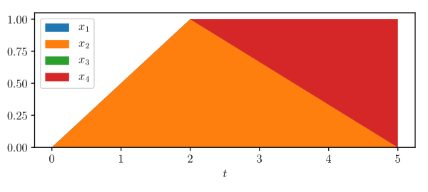
Figure 1: Basic feasible solutions for a subproblem with $m=4$ resources, with data (12), as $t$ varies. The first and third resources are never used.

We will now assume that the efficiencies are sorted and distinct, so $a_{1}<\cdots<a_{m}$. (The results given below are readily extended to the case when they are not distinct.) First suppose that $x_{i}$ and $x_{j}$ are nonzero, with $i<j$. (This corresponds to the case when the job uses only resources $i$ and $j$.) Then $s=0$, so $x_{i}+x_{j}=1$ and $a_{i}x_{i}+a_{j}x_{j}=t$, so

$$x_{i}=\frac{a_{j}-t}{a_{j}-a_{i}},\qquad x_{j}=\frac{t-a_{i}}{a_{j}-a_{i}}.$$ (13)

For these to be nonnegative, we must have $t\in[a_{i},a_{j}]$. The associated objective value is

$$p_{i}\frac{a_{j}-t}{a_{j}-a_{i}}+p_{j}\frac{t-a_{i}}{a_{j}-a_{i}}.$$ (14)

As $t$ varies between $a_{i}$ and $a_{j}$, this varies affinely between $p_{i}$ and $p_{j}$, respectively.

Now consider the special case when $x_{j}$ and $s$ are nonzero. (This corresponds to the case when the job uses only resource $j$.) Then we have $a_{j}x_{j}=t$, so

$$x_{j}=t/a_{j}.$$

For $x_{j}$ and $s=1-x_{j}$ to be nonnegative, we need $t\in[0,a_{j}]$. The corresponding objective value is

$$p_{j}t/a_{j}.$$

These are the same as the formulas (13) and (14) above, with $i=0$, where we define $a_{0}=p_{0}=0$.

The optimal value $c(t)$ is the pointwise minimum of the $m(m+1)/2$ affine functions, restricted to an interval,

$$p_{i}\frac{a_{j}-t}{a_{j}-a_{i}}+p_{j}\frac{t-a_{i}}{a_{j}-a_{i}}+\mathcal{I}(t\in[a_{i},a_{j}]),\quad i<j.$$

The graphs of these functions are line segments that connect the points $(a_{i},p_{i})$ and $(a_{j},p_{j})$, including the additional point $(a_{0},p_{0})=(0,0)$. The graph of $c(t)$ is the pointwise minimum of these. It is easy to see that $c$ is piecewise affine with kinks points that are a subset of the values $a_{1},\ldots,a_{m}$. It is increasing and convex, and satisfies $c(0)=0$, and has domain $[0,a_{m}]$.

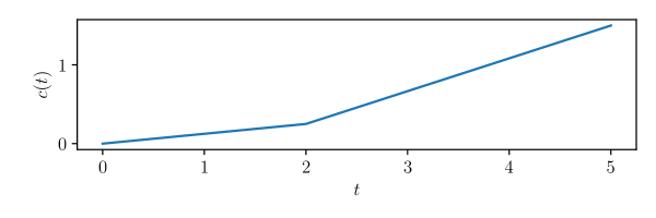
Figure 2: A graph of the piecewise affine optimal cost $c(t)$, for a fixed price vector and four resources.

Given $a$ and $p$, it is straightforward to directly compute the piecewise affine function $c$, i.e., to find its kink points and the slope in between successive kink points. It is completely specified by a subset of $\{0,\ldots,m\}$, given by $0=i_{1}<\cdots<i_{r}=m$. The kink points are $a_{i_{l}}$, $l=1,\ldots,r$, and the value of $c$ at these points is $p_{i_{l}}$.

This is illustrated in figure 2, for the same example as above with data (12). In this case the active subset is $0,2,4$, and $c$ is piecewise affine with kink points $0,a_{2}=2,a_{4}=5$, and associated values $0,p_{2}=1,p_{4}=6$.

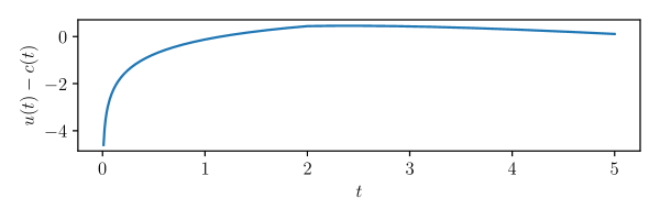
Figure 3: Net utility, i.e., utility minus cost, for a log utility and four resources.

4.2 Solving the subproblem

Once we have the explicit function $c$, we can readily solve the one dimensional problem (11). To do this we maximize $u$ minus an affine function over each of the intervals between successive kink points and choose the one with largest objective. Thus we need to maximize $u(t)-(\alpha t+\beta)$ over $t\in[\gamma,\delta]$, where $\alpha,\beta,\gamma,\delta$ are given, with $\alpha>0$. This is readily done for any utility function. For example, if $u$ is increasing and strictly concave (e.g., log utility) we have the explicit formula

$$t=\Pi(u^{\prime})^{-1}(\alpha),$$ (15)

where $\Pi$ is the projection onto the interval $[\gamma,\delta]$. (Since $u$ is strictly concave, $u^{\prime}$ is increasing and therefore invertible.) Figure 3 plots $u(t)-c(t)$ for our running example with $m=4$ resources, data (12), and log utility; in this case, a value of $t\approx 2.4$ is optimal.

This small problem is also easily solved for cases when the utility is neither increasing nor strictly concave, e.g., the target-priority utility (2). For this utility function, the solution is

$$t=\left\{\begin{array}[]{ll}t^{\text{des}}&w>\alpha,~{}\gamma\leq t^{\text{des}}\leq\delta,\\ \gamma&w\leq\alpha,\\ \delta&w>\alpha,~{}\delta\leq t^{\text{des}}.\end{array}\right.$$ (16)

Summary.

We summarize the algorithm for solving the job subproblem (2) below.

Algorithm 1 Maximizing net utility given prices $p\in{\mbox{\bf R}}^{m}_{+}$, efficiency vector $a\in{\mbox{\bf R}}^{m}_{+}$ ($a_{1}<a_{2}<\cdots<a_{m}$), utility function $u:{\mbox{\bf R}}\to{\mbox{\bf R}}$ 1. Compute $c(t)$. Compute the piecewise affine function $c$ as the pointwise minimum of $m(m+1)/2$ affine functions. 2. Compute optimal throughput. Compute the $t$ maximizing $u(t)-c(t)$ (e.g., via (15) or (16)) 3. Compute optimal allocation. Compute the allocation for the pair $(i,j)$ achieving the maximum net utility, as in (13). Note that we access the utility function $u$ in just two ways: we must be able to evaluate $u$ at any throughput $t$, and obtain the $t$ maximizing $u(t)-c(t)$.

Complexity.

The complexity of this method of solving the job subproblem is quadratic in $m$. By solving it in parallel for all $n$ jobs (in §6, we describe one way to parallelize these solves) , we go from a proposed resource price vector $p$ to an allocation that satisfies all constraints, except possibly the total resource usage limit. At the same time we can evaluate the dual function $g(p)$, and a subgradient of it, as described above.

5 Price discovery algorithm

Now we can give our method for solving the resource allocation problem (2). We will instead solve the dual problem (7), in order to discover the optimal resource prices; we recover an optimal allocation from solutions of the subproblems (5).

Our dual or price discovery algorithm adjusts the resource prices. We let $p^{k}\in{\mbox{\bf R}}_{+}^{m}$ denote the prices in iteration $k$. We first evaluate the dual function $g(p^{k})$ and a subgradient $q^{k}$. We do this by solving the subproblems as in §4 for each $i$, using algorithm 4.2, in parallel. This gives us an upper bound on $U^{\star}$, and a resource allocation $X^{k}$ that satisfies the job constraints $x_{i}\geq 0$ and $\mathbf{1}^{T}x_{i}\leq 1$, but need not satisfy the total resource usage limit $(X^{k})^{T}\mathbf{1}\leq R$.

From this allocation we create a feasible allocation, by scaling down each column of $X^{k}$ so that the resource usage limit holds. We refer to this feasible allocation as $\tilde{X}^{k}$. We evaluate its utility, which is a lower bound on $U^{\star}$. Thus we have lower and upper bounds on $U^{\star}$,

$$U(\tilde{X}^{k})\leq U^{\star}\leq g(p^{k}).$$

We refer to $g(p^{k})-U(\tilde{X}^{k})$ as the duality gap in iteration $k$. We quit when this is small, with a guarantee on how far from optimal the current allocation is.

Standard subgradient price update.

To move to the next iteration we update the prices. A standard subgradient method uses the projected gradient update

$$p^{k+1}=\max\{p^{k}-\alpha_{k}q^{k},0\},$$

where $\alpha_{k}$ are positive step lengths that satisfy $\alpha_{k}\to 0$ and $\sum_{k=1}^{\infty}\alpha_{k}=\infty$. This simple update guarantees convergence, i.e., $p^{k}\to p^{\star}$ [Sho85, BXM03]. It is also extremely intuitive. Recall that $q^{k}=R-r^{k}$, so that $-q^{k}$ tells us how much we are over-using the resources, i.e., $-q^{k}_{j}>0$ means that using the prices $p^{k}$, we have $r^{k}_{j}>R_{j}$. The subgradient update above says that we should increase the price for resources we are currently over-using, and decrease the price for any resource we are under-using (but never decrease a price below zero).

Recall that the optimal price vector gives the true prices of each resource, from which an optimal allocation is easily obtained (see §3).

More efficient price updates.

The projected subgradient method described above always works, even when $g$ is nondifferentiable. We can also use more efficient and sophisticated methods for minimizing $g$ that rely on $g$ being differentiable, for example a quasi-Newton method such as the BFGS method [Bro70, Fle70, Gol70, Sha70] or its limited memory variants [Noc80, LN89]. While $g$ need not be differentiable, for example with target-priority utility, it is quite smooth when $n$ is large, and we have observed no practical cases where it failed. (In any case, we can always fall back on the basic subgradient method.)

Initialization.

The initial price vector $p^{1}$ can be anything, including $0$ or $\mathbf{1}$. We have found a simple initialization that depends on the data ($a_{i}$, $R$, and $u_{i}$) and yields prices that are reasonably close to the optimal ones. We start with the simple allocation $x_{i}=(1/n)R$ for all $i$, which distributes the full usage budget uniformly across the jobs. (If $\kappa=\mathbf{1}^{T}(1/n)R>1$, we take $x_{i}=(1/(\kappa n)R$, so $\mathbf{1}^{T}x_{i}=1$.) We take as a starting price

$$p^{1}=\nabla_{R}U(R)=\frac{1}{n}\sum_{i=1}^{n}u_{i}^{\prime}(a_{i}^{T}x_{i})a_{i}.$$ (17)

(When $u_{i}$ is not differentiable, we can take a supergradient, i.e., the negative of a subgradient of $-u$.) This simple initialization is motivated by the observation that the optimal prices give the sensitivity of the total utility to the resource constraint [BV04, §5.6.3]. We have found it to work well in practice.

Algorithm summary.

We summarize our price discovery algorithm for solving the resource allocation problem (4) below.

Algorithm 2 Resource allocation price discovery given efficiency vectors $a_{i}\in{\mbox{\bf R}}^{m}_{+}$, utility functions $u_{i}:{\mbox{\bf R}}\to{\mbox{\bf R}}$, total resource usage limit $R$, initial resource prices $p^{1}\in{\mbox{\bf R}}_{+}^{m}$, tolerance $\epsilon>0$ For iteration $k=1,2,\ldots,K^{\text{max}}$ 1. With prices $p^{k}$, solve $n$ subproblems in parallel to find • allocation $X^{k}$ • dual function value $g(X^{k})$ • dual function gradient $q^{k}$ • feasible allocation utility value $U(\tilde{X}^{k})$ 2. Quit if $g(p^{k})-U(\tilde{X}^{k})\leq\epsilon$ 3. Update prices to obtain $p^{k+1}$

A reasonable choice of the tolerance $\epsilon$ is $10^{-3}n$, which guarantees that our final allocation is no more than $10^{-3}$ suboptimal in average utility. With log utility, this means the throughputs are optimal to within around 0.1%, which is far more than good enough for any practical application. (The algorithm can be run to much higher accuracy as well.)

6 Numerical examples

6.1 Implementation

We have implemented the price discovery algorithm 5 in PyTorch [Pas+19], along with an object-oriented interface for specifying and solving resource allocation problems of the form (4). In our library, users can select from a library of utility functions (or define their own). Our code is open-source, and available at

https://github.com/cvxgrp/resalloc.

Solving the subproblems in parallel.

Our implementation of algorithm 4.2 is completely vectorized and exploits the fact that for each subproblem, there is a basic feasible solution in which at most two resources are used. In particular, we compute the slopes of the affine functions on which $c(t)$ depends using vectorized operations (across all jobs), and collect them into a matrix of shape $n$ by $m(m-1)/2$ (this is tractable, because in the problems we are interested in $m\ll n$). We then operate on this matrix in a vectorized fashion to obtain the allocation solving the subproblem.

Roughly speaking, this means we solve the $n$ subproblems in parallel, but not by spawning multiple threads that solve the problems in isolation. Instead, we make heavy use of vector and matrix operations (avoiding control flow such as for loops as much as possible), and let our numerical linear algebra software (i.e., PyTorch) exploit the parallelism that is intrinsic to these operations. On a CPU, this means we exploit parallelism at multiple levels: the vector and matrix operations are split over multiple threads, and each thread in turn can take advantage of SIMD (single instruction, multiple data) operations supported by the hardware [HP11, Chap. 4]. Additionally, our software library supports CUDA acceleration via PyTorch, i.e., users can run the price discovery method on GPUs; in this case, the vector and matrix operations in our implementation are split over the GPU’s streaming multiprocessors, each of which can be thought of as a SIMD processor.

Because we efficiently exploit parallelism, our implementation is often orders of magnitude faster than off-the-shelf solvers for convex optimization, and it can scale to much larger problems. We will see some experiments that demonstrate this in the following subsections.

Utility functions.

Our implementation is modular, and can support any utility function that implements three specific methods: one that evaluates the utility, one that solves the subproblem (11) (given the slopes of the affine functions on which $c(t)$ depends), and one that computes an initial guess for the price vector (this guess need not be intelligent). These methods must be vectorized over jobs, which is simple to do using PyTorch.

Code example.

Below we show a code example that formulates a simple resource allocation problem using our software. (Here, the entries of the resource limits and throughput matrix are randomly generated; in an application, a user would use their real data for these variables.)

⬇

import torch

from resalloc.fungible import AllocationProblem, utilities

n_jobs, n_resources = int(1e6), 4

throughput_matrix = torch.rand((n_jobs, n_resources))

resource_limits = torch.rand(n_resources) * n_jobs + 1e3

problem = AllocationProblem(

throughput_matrix=throughput_matrix,

resource_limits=resource_limits,

utility_function=utilities.Log()

)

The problem can then be solved by calling the solve method:

⬇

problem.solve(verbose=True)

This yields the following verbose output, tracking the progress of the algorithm; each line prints the average utility, dual function value (divided by the number of jobs), and the gap between the two at a specific iteration of the price discovery algorithm. (By default the solver uses L-BFGS for the price updates, and terminates when the gap is less than $10^{-3}$.)

⬇

iteration 00 | utility=-0.349803 | dual_value=0.275906 | gap=6.26e-01

iteration 05 | utility=-0.274916 | dual_value=-0.26548 | gap=9.44e-03

Converged in 009 iterations, with residual 0.000161

After calling the solve method, the optimal allocation can be obtained by accessing the X attribute of the problem object (problem.X), and the optimal prices can be obtained via the prices attribute (problem.prices).

Solving this problem using a GPU requires just two changes to the code sample, shown below.

⬇

problem = AllocationProblem(

throughput_matrix=throughput_matrix.cuda(),

resource_limits=resource_limits.cuda(),

utility_function=utilities.Log()

Experiment set-up.

In the following subsections, we demonstrate our implementation on numerical examples. All experiments use our implementation with default parameter values and 32-bit floating points. We use L-BFGS with memory $10$ for the price updates, and we run the algorithms with tolerance $\epsilon=10^{-3}n$, which is more accuracy than needed in any practical application. We run the algorithm on a CPU, an Intel i7-6700K CPU with four physical cores clocked at 4 GHz, and also a GPU, an NVIDIA GeForce GTX 1070 with 1920 cores clocked at 1.5 GHz and a peak of 6.5 TFLOPs. We also give some experiments on a more compute-intensive configuration, an NVIDIA DGX-1 equipped with an NVIDIA Tesla V100 SXM2 GPU, which has 5120 cores clocked at 1.29 GHz and a peak of 15.7 TFLOPs.

Where possible, we cross check each solution found by our method using CVXPY [DB16, Agr+18] with the MOSEK solver [ApS21], a high performance commercial interior-point solver. (CVXPY is unable to compile one very large instance, and we suspect MOSEK would be unable to solve it on our machine.) In all cases, the allocations found using our method and MOSEK agreed.

6.2 A medium size problem

We consider a medium size problem, with $n=10^{6}$ jobs and $m=4$ resources. The data are synthetic but realistic. We choose the entries of $a_{i}$ from uniform distributions,

$$(a_{i})_{1}\sim U(0.1,0.3)\quad(a_{i})_{2}\sim U(0.1,0.5)\quad(a_{i})_{3}\sim U(0.3,0.8)\quad(a_{i})_{4}\sim U(0.6,1.0)$$

and we choose $R$ as

$$R=(8\times 10^{5},10^{5},10^{4},10^{3}),$$

so that the resources that are more efficient (on average) are also more scarce. We consider two problems, one with log utility and another with target-priority utility, with $t_{i}=0.2$ and priorities randomly chosen to be $w_{i}=1$ or $w_{i}=2$ (each with probability one half).

We ran the price discovery algorithm on these problems, using the initialization (17) for the prices. Maximizing the log utility took 3.9 seconds on our CPU and 0.30 seconds on our GPU; maximizing the target-priority utility took 11 seconds on our CPU and 0.89 seconds on our GPU. These are impressive solve times, considering our problem has 4 million variables. For comparison, MOSEK (which solves to high accuracy) took 300 seconds and 36 iterations for the log utility and 99 seconds and 74 iterations for the target-priority. MOSEK’s set-up time for the problems was 18 seconds and 13 seconds, respectively, and it it took MOSEK approximately 111 seconds and 85 seconds to reach solutions of the same accuracy as ours.

The progress of the algorithm is shown in figures 4 and 5, for the log and target-priority utilities, respectively. In each figure the top plot shows the prices $p^{k}$ versus iteration, with dashed lines showing the optimal prices $p^{\star}$. We can see that the prices converge to optimal (within $10^{-3}$) in 11 iterations for log utility and 21 iterations for target-priority utilities. The second plot shows the resource usage $r^{k}$ versus iteration, with dashed lines showing the resource limits. The resource usage constraints are violated early on but are satisfied by the end, as the prices converge to their optimal values. The third plot shows the upper and lower bounds on average utility, and the bottom plot shows the duality gap divided by $n$, $(g(X^{k})-U(\tilde{X}^{k}))/n$ (which is known at iteration $k$) and the true suboptimality divided by $n$, $(U^{\star}-U(\tilde{X}^{k}))/n$ (which is not known at iteration $k$). For $U^{\star}$ we used the optimal value obtained by MOSEK.

Figure 6 visualizes 50 rows of the optimal allocation matrices, along with the slack; the rows were selected by embedding the efficiency vectors $a_{i}$ into a line (using principal component analysis, via PyMDE [AAB21], a Python package for embedding), sorting the resulting embedding, and permuting the rows of the allocation matrix to match the sort order. For the allocation maximizing log utility, around 17 percent of jobs use two resources, the remaining use just one resource, and roughly 18 percent of jobs have a positive slack (meaning that $\mathbf{1}^{T}x_{i}<1$, i.e., these jobs would run for less than 100% total time). For the allocation maximizing the target-priority utility, 67 percent of jobs use two resources, the remaining use just one, and 50 percent have positive slack.

The job throughput distributions for the initial allocation, the allocation obtained after a few iterations, and the final optimal allocation $X^{\star}$ are shown for the two problems in figure 7. We can see that the target-priority allocation is able to obtain the target throughput $0.20$ for over 95% of the jobs. Figure 8 shows the throughput distributions for the target-priority optimal allocation, for the jobs with low priority ($w_{i}=1$) and higher priority ($w_{i}=2$), respectively. Virtually all of the high priority jobs achieve the target throughput, while around 10% of the low priority jobs do not. (Recall that roughly half the jobs are high priority, and half are low priority.)

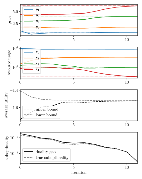
Figure 4: Log utility. Prices, resource usage, bounds on average log utility, and suboptimality versus iteration number.

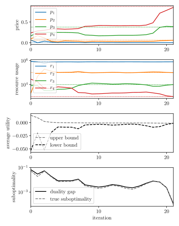
Figure 5: Target-priority utility. Prices, resource usage, bounds on average target-priority utility, and suboptimality versus iteration number.

Figure 6: Fifty rows of the optimal allocation matrices, along with the slack. Each row represents an allocation vector $x_{i}$, and each column a resource (or slack). Each job uses at most two resources. Top. Log utility. Bottom. Target-priority utility.

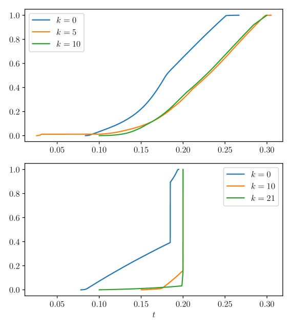
Figure 7: CDFs of throughputs, at various iteration numbers $k$. Top. Log utility. Bottom. Target-priority utility.

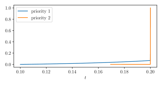
Figure 8: CDFs of throughputs for optimal target-priority allocations, for the low and high priority jobs.

6.3 A large problem

For our next example we consider a large problem with $n=50$ million jobs, $m=4$ resources, and log utility. This is a convex optimization problem with 200 million variables. We generate the entries of $a_{i}$ in the same way as the previous example, and use the previous resource limits scaled by 50.

We solved this problem on our smaller machine’s CPU, and on the Tesla V100 GPU (the problem was too large to fit on the smaller GPU). The problem was solved in 228 seconds on our CPU, and in roughly 7.9 seconds on the GPU. (This problem was too large to solve with MOSEK.) Figure 9 shows the progress of the algorithm. In the final allocation, 17 percent of jobs use two resources, the remaining use one, and 18 percent have positive slack.

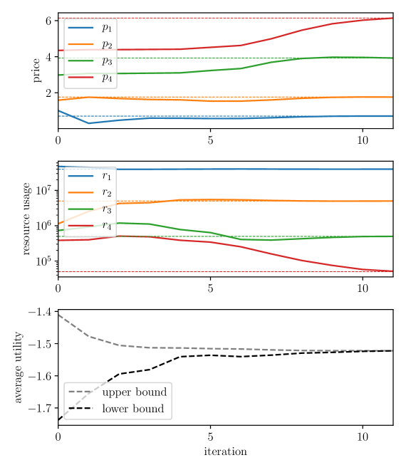
Figure 9: A large problem. Prices, resource usage, and bounds on average log utility versus iteration number, for a large problem with $n=50$ million jobs and $m=4$ resources. This problem was solved in 228 seconds on CPU and 7.9 seconds on GPU.

6.4 Scaling with jobs and resources

In this subsection we show how our method scales in the number of jobs and resources, and compare solve times for a number of problems against low-accuracy MOSEK solves.

Evaluating the dual function.

The main computation in each iteration of our algorithm is evaluating the dual function (i.e., solving the $n$ subproblems). To give an idea of how our implementation scales, we timed how long it took to evaluate the dual function for synthetic problems, varying the number of jobs $n$ and resources $m$. We conducted two experiments. In one, we held $n$ fixed at $10^{5}$, and varied $m$ from $2$ to $100$; in the other, we held $m$ fixed at $4$, and varied $n$ from $10^{2}$ to $10^{7}$. For each instance we evaluated the dual function five times. The mean times are plotted in figure 10. To study the scaling, for each plot we log-transformed the inputs and outputs and fit linear regressions, i.e., we fit models of the form

$$\log(s)\approx a+b\log(m),\quad\log(s)\approx a+b\log(n),$$

where $s$ is the elapsed time. We fit these models in ranges where the constant overhead of our software implementation no longer dominated. These fits are plotted as dashed lines in figure 10.

For CPU, the coefficient $b$ is 2.03 for resources and 1.05 for jobs; for GPU (we used the Tesla V100), $b$ is 1.75 for resources and 0.81 for jobs. (The coefficients $a$ are very small: for CPU, $\exp(a)$ is $1.4\times 10^{-3}$ and $1.6\times 10^{-7}$ for resources and jobs respectively, and for GPU the values are $6.7\times 10^{-5}$ and $1.7\times 10^{-7}$.) This means that CPU time scales quadratically in the number of resources and linearly in the number of jobs, while GPU times scales less than quadratically in the number of resources and sublinearly in the number of jobs, at least over the range considered.

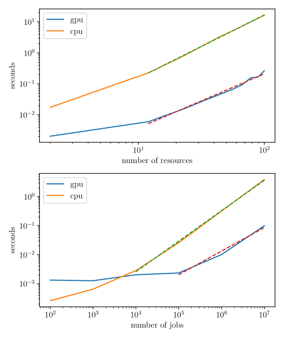
Figure 10: Evaluating the dual function. Mean time elapsed evaluating the dual function, with dashed lines showing scaling over ranges where the fixed overhead no longer dominates. Top. $n=10^{5}$, with $m$ varying. Bottom. $m=4$, with $n$ varying.

Comparison to MOSEK.

For large problems, our method outperforms high-quality off-the-shelf solvers for convex optimization, such as MOSEK. To demonstrate this, we timed how long it took our method to solve a number of synthetic problems (with log utility and accuracy $\epsilon=10^{-3}n$), varying the number of jobs $n$ and resources $m$; we solved the same problems with MOSEK, to low accuracy (setting all tolerances to $10^{-3}$). In the first set of experiments, we held $n$ fixed at $10^{6}$, and varied $m$ from $2$ to $16$; in the second, we held $m$ fixed at $4$, and varied $n$ from $10^{2}$ to $10^{6}$. The columns of the throughput matrices were sampled from uniform distributions, so that (on average) the resources were ordered from least to most efficient. The resource limits were generated by sampling each entry from a uniform distribution on $[0.1,1]$, and scaling the first component by the number of jobs, the second by the number of jobs divided by 1.5, the third by the number of jobs divided by $1.5^{2}$, and so on. We solved five instances of each problem.

The mean solve times are plotted in figure 11. For large problems, our method appears to be between one to three orders of magnitude faster than low-accuracy MOSEK solves. We point out that we solve the largest instance, which has 16 million variables ($n=10^{6}$ jobs and $m=16$ resources), in just 5 seconds on a GPU. On this same instance, MOSEK takes over 200 seconds.

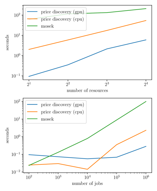
Figure 11: Comparison to MOSEK. Mean time elapsed solving resource allocation problems with log utility, comparing our method and low-accuracy MOSEK solves. Top. $n=10^{6}$, with $m$ varying. Bottom. $m=4$, with $n$ varying.

7 Conclusion

We have described a custom solver for the fungible resource allocation problem that scales to extremely large problem instances, especially when run on a GPU. For example, problems with millions of variables can be solved in well under a second. Smaller problems can be solved in milliseconds.

The method uses the dual problem, and manipulates a set of resource prices until we achieve an optimal allocation. The optimal prices, which our algorithm discovers, can be used for other tasks as well as a solving the allocation problem. For example we can actually charge jobs in proportion to $(p^{\star})^{T}x_{i}$, the total cost of the resources used with the optimal prices.

The prices can also be used in situations where an allocation problem is broken into $M$ shards or subproblems, and each of these solved independently with resource budget $(1/M)R$ (as proposed in [Nar+21]). If the optimal resource prices for the different shards are close, we can conclude that the solution found from the partitioned problems is nearly optimal for the allocation problem, had they been solved together. If the resource prices vary across the shards, they can be used to re-allocate resources to the shards, by moving resources from the shards with lower prices to those with higher prices. This method, which is very interpretable, can be shown to converge to the solution of the larger problem [Boy+07, §3.1], and it can be used to improve suboptimal solutions obtained via the method from [Nar+21]. This method could also be used to re-allocate resources across separate virtual data centers in a principled way.

7.1 Extensions and variations

We mention a few extensions and variations on our method, and related problems. The first is the min-throughput utility. This objective function is concave and nondecreasing, but it is not separable, so the methods of this paper cannot be directly used. But very similar methods can be. Methods described in this paper can be used to approximate the min-throughput utility; for example, just using a utility function with strong curvature, like a power utility with $p$ near zero, already gives a good approximation of the minimum throughput. Or we can use a target-priority utility and decrease the target throughput until all (or a large fraction) of the jobs meet the target.

Our formulation (4) can easily be extended to the case in the constraint on the resource usage is replaced with $\sum_{i=1}^{n}d_{i}x_{i}\leq R$, where $d_{i}\in{\mbox{\bf R}}_{++}$ is the number of resources demanded by job $i$ (this constraint was proposed in [Nar+20]). For example, if $d_{i}=2$, and the resources are GPUs, this means that job $i$ requires two GPUs in order to run. We can also handle the case in which jobs demand different amounts of different resources (leading to demands that are vectors in ${\mbox{\bf R}}^{m}_{++}$, not scalars). These extensions would require very minimal changes to our price discovery method (the only change is that the price vector in each subproblem (10) is multiplied by the job’s demand); indeed, we have implemented them in our software.

In this paper we only considered the problem of allocating the fraction of time that a job should spend consuming each resource; we did not consider the problem of coming up with a schedule, which says when each job should consume its resources during the time interval. In our motivating application of computer systems, some pairs of jobs exhibit poor performance when colocated on the same hardware (i.e., when using the same resource) [Kam+12, Zha+13, Ver+15, Nar+20]. This kind of interference could be mitigated by a lower-level scheduler, which takes as input an optimal allocation matrix, and comes up with a concrete schedule that respects the time-slicing while minimizing cross-job interference. The lower-level scheduler could itself be based on solving an optimization problem; Netflix’s optimization-based scheduler is one such example [RH19]. We mention that it is also possible to take interference into account in a higher-level optimization-based scheduler, possibly using a formulation of the resource allocation problem that is different from ours (one such formulation is given in [Nar+20, §3.1]).

Finally, another related and important problem is the allocation of non-fungible resources. This occurs when the resources are heterogeneous, and not fully exchangeable. For example in a data center, we can allocate number of cores, I/O bandwidth, memory, and disk space. (These are not fungible, because you cannot get any throughput if you only use I/O bandwidth and no cores, memory, or disk space.) In this setting, the utility function for each job does not have the form of a scalar utility function of a linear function of the resources allocated; instead it is a utility function of $x_{i}$. These problems can often be posed as convex optimization problems (e.g., [Gho+11, BS11].) The specific solution of the subproblem described in §4 no longer applies, but the price discovery method in general does. We will address that problem in a future paper.

References

- [AAB21] Akshay Agrawal, Alnur Ali and Stephen Boyd “Minimum-distortion embedding” In arXiv, 2021
- [Agr+19] Akshay Agrawal, Brandon Amos, Shane Barratt, Stephen Boyd, Steven Diamond and J Zico Kolter “Differentiable Convex Optimization Layers” In Advances in Neural Information Processing Systems, 2019, pp. 9558–9570
- [Agr+18] Akshay Agrawal, Robin Verschueren, Steven Diamond and Stephen Boyd “A rewriting system for convex optimization problems” In Journal of Control and Decision 5.1, 2018, pp. 42–60
- [ApS21] MOSEK ApS “MOSEK optimization suite”, http://docs.mosek.com/9.2/intro.pdf, 2021
- [Arr71] Kenneth Arrow “Essays in the Theory of Risk-Bearing” Markham Publishing Company, 1971
- [Ban+17] Goran Banjac, Bartolomeo Stellato, Nicholas Moehle, Paul Goulart, Alberto Bemporad and Stephen Boyd “Embedded Code Generation Using the OSQP Solver” In IEEE Conference on Decision and Control, 2017
- [Ber99] D Bertsekas “Nonlinear Programming” Athena Scientific, 1999
- [BGH92] Dimitri Bertsekas, Robert Gallager and Pierre Humblet “Data Networks” Prentice-Hall International New Jersey, 1992
- [BT97] Dimitris Bertsimas and John Tsitsiklis “Introduction to Linear Optimization” Athena Scientific, 1997
- [BS11] Sarah Bird and Burton Smith “PACORA: Performance aware convex optimization for resource allocation” In Proceedings of the 3rd USENIX Workshop on Hot Topics in Parallelism, 2011
- [Bla16] Lars Blackmore “Autonomous Precision Landing of Space Rockets” In The BRIDGE 26.4 National Academy of Engineering, 2016
- [BCS84] Roger Bohn, Michael Caramanis and Fred Schweppe “Optimal pricing in electrical networks over space and time” In The RAND Journal of Economics JSTOR, 1984, pp. 360–376
- [BV04] Stephen Boyd and Lieven Vandenberghe “Convex Optimization” New York, NY, USA: Cambridge University Press, 2004
- [BXM03] Stephen Boyd, Lin Xiao and Almir Mutapcic “Subgradient methods” Lecture notes for the course Convex Optimization II, 2003
- [Boy+07] Stephen Boyd, Lin Xiao, Almir Mutapcic and Jacob Mattingley “Notes on decomposition methods” Lecture notes for the course Convex Optimization II, 2007
- [Bro70] Charles George Broyden “The convergence of a class of double-rank minimization algorithms, general considerations” In IMA Journal of Applied Mathematics 6.1 Oxford University Press, 1970, pp. 76–90
- [BRB16] Enzo Busseti, Ernest Ryu and Stephen Boyd “Risk-constrained Kelly gambling” In The Journal of Investing 25.3, 2016, pp. 118–134
- [Chi+07] Mung Chiang, Steven Low, A Robert Calderbank and John Doyle “Layering as optimization decomposition: A mathematical theory of network architectures” In Proceedings of the IEEE 95.1 IEEE, 2007, pp. 255–312
- [Chu+13] Eric Chu, Neal Parikh, Alexander Domahidi and Stephen Boyd “Code generation for embedded second-order cone programming” In European Control Conference, 2013, pp. 1547–1552 IEEE
- [DB16] Steven Diamond and Stephen Boyd “CVXPY: A Python-embedded modeling language for convex optimization” In Journal of Machine Learning Research 17.1 JMLR. org, 2016, pp. 2909–2913
- [DCB13] Alexander Domahidi, Eric Chu and Stephen Boyd “ECOS: An SOCP solver for embedded systems” In European Control Conference, 2013, pp. 3071–3076 IEEE
- [EGS11] Louis Eeckhoudt, Christian Gollier and Harris Schlesinger “Economic and Financial Decisions under Risk” Princeton University Press, 2011
- [FS06] Erlon Cristian Finardi and Edson Luiz Silva “Solving the hydro unit commitment problem via dual decomposition and sequential quadratic programming” In IEEE Transactions on Power Systems 21.2 IEEE, 2006, pp. 835–844
- [Fle70] Roger Fletcher “A new approach to variable metric algorithms” In The Computer Journal 13.3 Oxford University Press, 1970, pp. 317–322
- [FS48] Milton Friedman and L. Savage “The Utility Analysis of Choices Involving Risk” In Journal of Political Economy 56.4, 1948, pp. 279–304
- [Gho+11] Ali Ghodsi, Matei Zaharia, Benjamin Hindman, Andy Konwinski, Scott Shenker and Ion Stoica “Dominant resource fairness: Fair allocation of multiple resource types” In 8th USENIX Symposium on Networked Systems Design and Implementation (NSDI 20) 11.2011, 2011, pp. 24–24
- [Gol70] Donald Goldfarb “A family of variable-metric methods derived by variational means” In Mathematics of Computation 24.109, 1970, pp. 23–26
- [Gol01] Christian Gollier “The Economics of Risk and Time” MIT press, 2001
- [HP11] John Hennessy and David Patterson “Computer Architecture: A Quantitative Approach” Morgan Kaufmann Publishers Inc., 2011
- [HUL93] Jean-Baptiste Hiriart-Urruty and Claude Lemaréchal “Convex Analysis and Minimization Algorithms. II” Advanced theory and bundle methods 306, Grundlehren der Mathematischen Wissenschaften [Fundamental Principles of Mathematical Sciences] Springer-Verlag, Berlin, 1993
- [Hu+18] Mian Hu, Jiang-Wen Xiao, Shi-Chang Cui and Yan-Wu Wang “Distributed real-time demand response for energy management scheduling in smart grid” In International Journal of Electrical Power & Energy Systems 99 Elsevier, 2018, pp. 233–245
- [Kam+12] Melanie Kambadur, Tipp Moseley, Rick Hank and Martha Kim “Measuring interference between live datacenter applications” In Proceedings of the International Conference on High Performance Computing, Networking, Storage and Analysis (SC’12), 2012, pp. 1–12 IEEE
- [KMT98] Frank Kelly, Aman Maulloo and David Tan “Rate control for communication networks: Shadow prices, proportional fairness and stability” In Journal of the Operational Research Society 49.3 Taylor & Francis, 1998, pp. 237–252
- [KJ56] John Kelly Jr “A new interpretation of information rate” In IRE Transactions on Information Theory 2.3, 1956, pp. 185–189
- [KPT07] Nikos Komodakis, Nikos Paragios and Georgios Tziritas “MRF optimization via dual decomposition: Message-passing revisited” In 2007 IEEE 11th International Conference on Computer Vision, 2007, pp. 1–8 IEEE
- [LN89] Dong Liu and Jorge Nocedal “On the limited memory BFGS method for large scale optimization” In Mathematical Programming 45.1-3 Springer, 1989, pp. 503–528
- [MTZ11] Leonard MacLean, Edward Thorp and WilliaT Ziemba “The Kelly Capital Growth Investment Criterion: Theory and Practice” World Scientific, 2011
- [Mar52] Harry Markowitz “Portfolio Selection” In The Journal of Finance 7.1, 1952, pp. 77–91
- [MB12] Jacob Mattingley and Stephen Boyd “CVXGEN: A code generator for embedded convex optimization” In Optimization and Engineering 13.1, 2012, pp. 1–27
- [MW00] Jeonghoon Mo and Jean Walrand “Fair end-to-end window-based congestion control” In IEEE/ACM Transactions on Networking 8.5 IEEE, 2000, pp. 556–567
- [Nar+21] Deepak Narayanan, Fiodar Kazhamiaka, Firas Abuzaid, Peter Kraft and Matei Zaharia “Don’t give up on large optimization problems; POP them!” In arXiv, 2021
- [Nar+20] Deepak Narayanan, Keshav Santhanam, Fiodar Kazhamiaka, Amar Phanishayee and Matei Zaharia “Heterogeneity-aware cluster scheduling policies for deep learning workloads” In 14th USENIX Symposium on Operating Systems Design and Implementation (OSDI 20), 2020, pp. 481–498
- [Noc80] Jorge Nocedal “Updating quasi-Newton matrices with limited storage” In Mathematics of Computation 35.151, 1980, pp. 773–782
- [PC06] Daniel Pérez Palomar and Mung Chiang “A tutorial on decomposition methods for network utility maximization” In IEEE Journal on Selected Areas in Communications 24.8 IEEE, 2006, pp. 1439–1451
- [Pas+19] Adam Paszke, Sam Gross, Francisco Massa, Adam Lerer, James Bradbury, Gregory Chanan, Trevor Killeen, Zeming Lin, Natalia Gimelshein and Luca Antiga “PyTorch: An imperative style, high-performance deep learning library” In Advances in Neural Information Processing Systems, 2019, pp. 8024–8035
- [Pra64] John Pratt “Risk Aversion in the Small and in the Large” In Econometrica 32.1/2, 1964, pp. 122–136
- [Ran09] Anders Rantzer “Dynamic dual decomposition for distributed control” In 2009 American Control Conference, 2009, pp. 884–888 IEEE
- [Roc70] R Rockafellar “Convex Analysis” Princeton University Press, 1970
- [RH19] Benoit Rostykus and Gabriel Hartman “Predictive CPU isolation of containers at Netflix”, 2019 URL: https://medium.com/netflix-techblog/predictive-cpu-isolation-of-containers-at-netflix-91f014d856c7
- [STA09] Peter Schütz, Asgeir Tomasgard and Shabbir Ahmed “Supply chain design under uncertainty using sample average approximation and dual decomposition” In European Journal of Operational Research 199.2 Elsevier, 2009, pp. 409–419
- [Sha70] David Shanno “Conditioning of quasi-Newton methods for function minimization” In Mathematics of Computation 24.111, 1970, pp. 647–656
- [Sho85] Naum Shor “Minimization Methods for Non-Differentiable Functions” Translated from Russian by K. Kiwiel and A. Ruszczyński 3, Springer Series in Computational Mathematics Springer-Verlag, 1985
- [Ste+20] Bartolomeo Stellato, Goran Banjac, Paul Goulart, Alberto Bemporad and Stephen Boyd “OSQP: An Operator Splitting Solver for Quadratic Programs” In Mathematical Programming Computation, 2020
- [Tob58] James Tobin “Liquidity preference as behavior towards risk” In The Review of Economic Studies 25.2 JSTOR, 1958, pp. 65–86
- [Tob+65] James Tobin “The theory of portfolio selection” In The Theory of Interest Rates 364 Macmillan London, 1965, pp. 364
- [Tum+16] Alexey Tumanov, Timothy Zhu, Jun Woo Park, Michael Kozuch, Mor Harchol-Balter and Gregory Ganger “TetriSched: Global rescheduling with adaptive plan-ahead in dynamic heterogeneous clusters” In Proceedings of the Eleventh European Conference on Computer Systems, 2016, pp. 1–16
- [Ver+15] Abhishek Verma, Luis Pedrosa, Madhukar Korupolu, David Oppenheimer, Eric Tune and John Wilkes “Large-scale cluster management at Google with Borg” In Proceedings of the Tenth European Conference on Computer Systems, 2015, pp. 1–17
- [WB10] Yang Wang and Stephen Boyd “Fast evaluation of quadratic control-Lyapunov policy” In IEEE Transactions on Control Systems Technology 19.4 IEEE, 2010, pp. 939–946
- [XJB04] Lin Xiao, Mikael Johansson and Stephen P Boyd “Simultaneous routing and resource allocation via dual decomposition” In IEEE Transactions on Communications 52.7 IEEE, 2004, pp. 1136–1144
- [YL06] Wei Yu and Raymond Lui “Dual methods for nonconvex spectrum optimization of multicarrier systems” In IEEE Transactions on Communications 54.7 IEEE, 2006, pp. 1310–1322
- [Zha+13] Xiao Zhang, Eric Tune, Robert Hagmann, Rohit Jnagal, Vrigo Gokhale and John Wilkes “: CPU performance isolation for shared compute clusters” In Proceedings of the 8th ACM European Conference on Computer Systems, 2013, pp. 379–391
- [ZGG13] Yu Zhang, Nikolaos Gatsis and Georgios B Giannakis “Robust energy management for microgrids with high-penetration renewables” In IEEE Transactions on Sustainable Energy 4.4 IEEE, 2013, pp. 944–953