Nonlinear optimized Schwarz preconditioner for elliptic optimal control problems

1 Introduction

Consider the nonlinear optimal control problem

$$\begin{split}\min_{y,u}&\;J(y,u):=\frac{1}{2}\|y-y_{d}\|_{L^{2}}^{2}+\frac{\nu}{2}\|u\|_{L^{2}}^{2}+\beta\|u\|_{L^{1}},\\ \text{s.t. }&-\Delta y+cy+b\varphi(y)=f+u\text{ in $\Omega$},\>y=0\text{ on $\partial\Omega$},\\ &u\in U_{\rm ad}:=\{v\in L^{2}(\Omega)\,:\,|v|\leq\bar{u}\text{ in $\Omega$}\},\end{split}$$ (1)

where $\|\cdot\|_{L^{r}}$ denotes the usual norm for $L^{r}(\Omega)$ with $1\leq r\leq\infty$, the functions $y_{d},f\in L^{2}(\Omega)$ are given, and the scalar parameters $b,c,\beta\geq 0$ and $\nu,\beta\geq 0$ are known. Our model includes problems such as the simplified Ginzburg-Landau superconductivity equation as well as inverse problems where $L^{1}$-regularization is used to enhance sparsity of the control function $u$. For simplicity, the domain $\Omega\subset\mathbb{R}^{2}$ is assumed to be a rectangle $(0,\widetilde{L})\times(0,\widehat{L})$. The function $\varphi:\mathbb{R}\rightarrow\mathbb{R}$ is assumed to be of class $C^{2}$, with locally bounded and locally Lipschitz second derivative and such that $\partial_{y}\varphi(y)\geq 0$. These assumptions guarantee that the Nemytskii operator $y(\cdot)\mapsto\varphi(y(\cdot))$ is twice continuously Fréchet differentiable in $L^{\infty}(\Omega)$. In this setting, the optimal control problem (1) is well posed in the sense that there exists a minimizer $(y,u)\in X\times L^{2}(\Omega)$, with $X:=H^{1}_{0}(\Omega)\cap L^{\infty}(\Omega)$, cf. troltzsch2010optimal ; Herzog . Our goal is to derive efficient nonlinear preconditioners for solving (1) using domain decomposition techniques.

Let $(y,u)\in X\times L^{2}(\Omega)$ be a solution to (1). Then there exists an adjoint variable $p\in X$ such that $(y,u,p)$ satisfies the system (Stadler2009, , Theorem 2.3)

$$-\Delta y+cy+b\varphi(y) =f+u \text{in $\Omega$ with $y=0$ on $\partial\Omega$},$$

$$-\Delta p+cp+b\varphi^{\prime}(y)p =y-y_{d} \text{in $\Omega$ with $p=0$ on $\partial\Omega$},$$

$$u =\mu(p),$$

where $\mu:L^{\infty}(\Omega)\rightarrow L^{2}(\Omega)$ is

$$\begin{split}\mu(p)=&\max(0,(-\beta-p)/\nu)+\min(0,(\beta-p)/\nu)\\ &-\max(0,-\bar{u}+(-p-\beta)/\nu)-\min(0,\bar{u}+(-p+\beta)/\nu).\end{split}$$ (2)

We remark that for $\beta=0$, the previous formula becomes $\mu(p)=\mathbb{P}_{U_{\rm ad}}(-p/\nu)$, which is the usual projection formula that leads to the optimality condition $u=\mathbb{P}_{U_{\rm ad}}(-p/\nu)$; see troltzsch2010optimal . Moreover, if $\beta=0$ with $\bar{u}=\infty$, one obtains that $\mu(p)=-p/\nu$, which implies the usual optimality condition $\nu u+p=0$, where $\nu u+p$ is the gradient of the reduced cost functional $\widehat{J}(u)=J(y(u),u)$ troltzsch2010optimal .

Eliminating the control using $\mu(p)$, the first-order optimality system becomes

$$\begin{split}-\Delta y+cy+b\varphi(y)&=f+\mu(p)\text{ in $\Omega$ with $y=0$ on $\partial\Omega$},\\ -\Delta p+cp+b\varphi^{\prime}(y)(p)&=y-y_{d}\quad\text{ in $\Omega$ with $p=0$ on $\partial\Omega$}.\end{split}$$ (3)

This nonlinear and nonsmooth system admits a solution $(y,p)\in X^{2}$ Herzog ; troltzsch2010optimal .

2 Optimized Schwarz method and preconditioner

In this section, we introduce an optimized Schwarz method (OSM) for solving the optimality system (3).

Figure 1: Non-overlapping domain decomposition.

We consider the non-overlapping decomposition of $\Omega$ shown in Fig. 1 and given by disjoint subdomains $\Omega_{j}$, $j=1,\dots,N$ such that $\overline{\Omega}=\cup_{j=1}^{N}\overline{\Omega}_{j}$. The sets $\Gamma_{j}:=\overline{\Omega}_{j}\cap\overline{\Omega}_{j+1}$, $j=1,\dots,N-1$ are the interfaces. Moreover, we define $\Gamma_{j}^{\rm ext}:=\partial\Omega_{j}\cap\partial\Omega$, $j=1,\dots,N$, which represent the external boundaries of the subdomains. The optimality system (3) can be written as a coupled system of $N$ subproblems defined on the subdomains $\Omega_{j}$, $j=1,\dots,N$, of the form

$$-\Delta y_{j}+cy_{j}+b\varphi(y_{1}) =f_{j}+\mu(p_{j}) \text{ in $\Omega_{j}$},$$ (4a)

$$-\Delta p_{j}+cp_{j}+b\varphi^{\prime}(y_{j})(p_{j}) =y_{j}-y_{d,j} \Omega_{j}$$ in (4b)

$$y_{j} =0,\;p_{j}=0 \text{ on $\Gamma_{j}^{\rm ext}$},$$ (4c)

$$q\,y_{j}+\partial_{x}y_{j} =q\,y_{j+1}+\partial_{x}y_{j+1} \text{ on $\Gamma_{j}$},$$ (4d)

$$q\,p_{j}+\partial_{x}p_{j} =q\,p_{j+1}+\partial_{x}p_{j+1} \text{ on $\Gamma_{j}$},$$ (4e)

$$q\,y_{j}-\partial_{x}y_{j} =q\,y_{j-1}-\partial_{x}y_{j-1} \text{ on $\Gamma_{j-1}$},$$ (4f)

$$q\,p_{j}-\partial_{x}p_{j} =q\,p_{j-1}-\partial_{x}p_{j-1} \text{ on $\Gamma_{j-1}$},$$ (4g)

for $j=1,\dots,N$, where for $j\in\{1,N\}$ the boundary conditions at $\Gamma_{0}$ and $\Gamma_{N}$, respectively, must be replaced with homogeneous Dirichlet conditions. Here, $q>0$ is a parameter that can be optimized to improve the convergence of the OSM; see, e.g, Gander2006 ; Chaouqui2018 . The system (4) leads to the OSM, which, for a given $(y_{j}^{0},p_{j}^{0})_{j=1}^{N}$, is defined by solving the subdomain problems

$$-\Delta y_{j}^{k}+cy_{j}^{k}+b\varphi(y_{1}^{k}) =f_{j}+\mu(p_{j}^{k}) \text{ in $\Omega_{j}$},$$ (5a)

$$-\Delta p_{j}^{k}+cp_{j}^{k}+b\varphi^{\prime}(y_{j}^{k})(p_{j}^{k}) =y_{j}^{k}-y_{d,j} \Omega_{j}$$ in (5b)

$$y_{j}^{k} =0,\;p_{j}^{k}=0 \text{ on $\Gamma_{j}^{\rm ext}$},$$ (5c)

$$q\,y_{j}^{k}+\partial_{x}y_{j}^{k} =q\,y_{j+1}^{k-1}+\partial_{x}y_{j+1}^{k-1} \text{ on $\Gamma_{j}$},$$ (5d)

$$q\,p_{j}^{k}+\partial_{x}p_{j}^{k} =q\,p_{j+1}^{k-1}+\partial_{x}p_{j+1}^{k-1} \text{ on $\Gamma_{j}$},$$ (5e)

$$q\,y_{j}^{k}-\partial_{x}y_{j}^{k} =q\,y_{j-1}^{k-1}-\partial_{x}y_{j-1}^{k-1} \text{ on $\Gamma_{j-1}$},$$ (5f)

$$q\,p_{j}^{k}-\partial_{x}p_{j}^{k} =q\,p_{j-1}^{k-1}-\partial_{x}p_{j-1}^{k-1} \Gamma_{j-1}$$ on (5g)

for $k\in\mathbb{N}^{+}$. Now, we use the OSM to introduce a nonlinear preconditioner by setting ${\bf y}_{j}:=(y_{j},p_{j})$, $j=1,\dots,N$, and defining the solution maps $S_{j}$ as

$$S_{1}({\bf y}_{2}) ={\bf y}_{1} \text{solution to \eqref{eq:sub1} with $j=1$ and ${\bf y}_{2}$ given},$$

$$S_{j}({\bf y}_{j-1},{\bf y}_{j+1}) ={\bf y}_{j} \text{solution to \eqref{eq:sub1} with $2\leq j\leq N-1$ and ${\bf y}_{j-1},{\bf y}_{j+1}$ given},$$

$$S_{N}({\bf y}_{N-1}) ={\bf y}_{N} \text{solution to \eqref{eq:sub1} with $j=N$ and ${\bf y}_{N-1}$ given}.$$

Hence, using the variable ${\bf y}=({\bf y}_{1},\dots,{\bf y}_{N})$, we can rewrite (4) as

$$\mathcal{F}_{\rm P}({\bf y})=0\text{, }\quad\text{where}\quad\mathcal{F}_{\rm P}({\bf y}):=\small\begin{bmatrix}{\bf y}_{1}-S_{1}({\bf y}_{2})\\ {\bf y}_{2}-S_{2}({\bf y}_{1},{\bf y}_{3})\\ \vdots\\ {\bf y}_{N-1}-S_{N-1}({\bf y}_{N-2},{\bf y}_{N})\\ {\bf y}_{N}-S_{N}({\bf y}_{N-1})\\ \end{bmatrix}.$$ (6)

This is the nonlinearly preconditioned form of (3) induced by the OSM (4)-(5), to which we can apply a generalized Newton method. For a given initialization ${\bf y}^{0}$, a Newton method generates a sequence $({\bf y}^{k})_{k\in\mathbb{N}}$ defined by

$$\text{solve }\quad D\mathcal{F}_{\rm P}({\bf y}^{k})({\bf d}^{k})=-\mathcal{F}_{\rm P}({\bf y}^{k})\quad\text{ and update }\quad{\bf y}^{k+1}={\bf y}^{k}+{\bf d}^{k}.$$ (7)

Notice that at each iteration of (7) one needs to evaluate the residual function $\mathcal{F}_{\rm P}({\bf y}^{k})$, which requires the (parallel) solution of the $N$ subproblems (4). The computational cost is therefore equivalent to one iteration of the OSM (5). As an inner solver for the subproblems, which involve the (mildly) non-differentiable function $\mu$, a semi-smooth Newton can be employed.

We now discuss the problem of solving the Jacobian linear system in (7). Let ${\bf d}=({\bf d}_{1},\dots,{\bf d}_{N})$, where ${\bf d}_{j}=(d_{y,j},d_{p,j})$, $j=1,\dots,N$. Then a direct calculation (omitted for brevity) shows that the action of the operator $D\mathcal{F}_{\rm P}({\bf y})$ on the vector ${\bf d}$ is given by $D\mathcal{F}_{\rm P}({\bf y})({\bf d})={\bf d}-\widetilde{{\bf y}}({\bf d})$, where $\widetilde{{\bf y}}:=(\widetilde{{\bf y}}_{1},\dots,\widetilde{{\bf y}}_{N})$, and each $\widetilde{{\bf y}}_{j}=(\widetilde{y}_{j},\widetilde{p}_{j})$ satisfies the linearized subdomain problems

$$-\Delta\widetilde{y}_{j}+c\widetilde{y}_{j}+b\varphi^{\prime}(y_{j})\widetilde{y}_{j} =D\mu(p_{j})(\widetilde{p}_{j}) \text{ in $\Omega_{j}$},$$ (8a)

$$-\Delta\widetilde{p}_{j}+c\widetilde{p}_{j}+b\varphi^{\prime\prime}(y_{j})[p_{j},\widetilde{y}_{j}] =\widetilde{y}_{j} \Omega_{j}$$ in (8b)

$$\widetilde{y}_{j} =0,\widetilde{p}_{j}=0 \text{ on $\Gamma_{j}^{\rm ext}$},$$ (8c)

$$q\,\widetilde{y}_{j}+\partial_{x}\widetilde{y}_{j} =q\,d_{y,j+1}+\partial_{x}d_{y,j+1} \text{ on $\Gamma_{j}$},$$ (8d)

$$q\,\widetilde{p}_{j}+\partial_{x}\widetilde{p}_{j} =q\,d_{p,j+1}+\partial_{x}d_{p,j+1} \text{ on $\Gamma_{j}$},$$ (8e)

$$q\,\widetilde{y}_{j}-\partial_{x}\widetilde{y}_{j} =q\,d_{y,j-1}-\partial_{x}d_{y,j-1} \text{ on $\Gamma_{j-1}$},$$ (8f)

$$q\,\widetilde{p}_{j}-\partial_{x}\widetilde{p}_{j} =q\,d_{p,j-1}-\partial_{x}d_{p,j-1} \text{ on $\Gamma_{j-1}$},$$ (8g)

where

$$\begin{split}D\mu(p)(\widetilde{p})=&\frac{1}{\nu}\Bigl{[}-\mathcal{G}_{\max}(-\beta-p)-\mathcal{G}_{\min}(\beta-p)\\ &+\mathcal{G}_{\max}(-p-\beta-\nu\bar{u})+\mathcal{G}_{\min}(-p+\beta+\nu\bar{u})\Bigr{]}\widetilde{p},\end{split}$$

with $\mathcal{G}_{\max}(v)(x)=\begin{cases}1&\text{if $v(x)>0$},\\ 0&\text{if $v(x)\leq 0$},\\ \end{cases}$ and $\mathcal{G}_{\min}(v)(x)=\begin{cases}1&\text{if $v(x)\leq 0$},\\ 0&\text{if $v(x)>0$},\\ \end{cases}$
and where the boundary values for $j\in\{1,N\}$ have to be modified as in (4).

Note that this is the same linearized problem that must be solved repeatedly within the inner iterations of semi-smooth Newton, so its solution cost is only a fraction of the cost required to calculate $\mathcal{F}_{\rm P}({\bf y})$.

We are now ready to state our matrix-free preconditioned semismooth Newton algorithm that corresponds to the Newton procedure (7).

Algorithm 1 Matrix-free preconditioned generalized Newton method

0:  Initial guess ${\bf y}^{0}$, tolerance $\epsilon$, maximum number of iterations $k_{\max}$.

1:  Compute $S_{1}({\bf y}_{2}^{0})$, $S_{j}({\bf y}_{j-1}^{0},{\bf y}_{j+1}^{0})$, $j=2,\dots,N-1$, and $S_{N}({\bf y}_{N-1}^{0})$.

2:  Set $k=0$ and assemble $\mathcal{F}_{\rm P}({\bf y}^{0})$ using (6).

3:  while $\|\mathcal{F}_{\rm P}({\bf y}^{k})\|\geq\epsilon$ and $k\leq k_{\max}$ do

4:     Compute ${\bf d}^{k}$ by solving $D\mathcal{F}_{\rm P}({\bf y}^{k})({\bf d}^{k})=-\mathcal{F}_{\rm P}({\bf y}^{k})$ using a matrix-free Krylov method, e.g., GMRES (together with a routine for solving (8) to compute the action of $D\mathcal{F}_{\rm P}({\bf y}^{k})$ on a vector ${\bf d}$).

5:     Update ${\bf y}^{k+1}={\bf y}^{k}+{\bf d}^{k}$.

6:     Set $k=k+1$.

7:     Compute $S_{1}({\bf y}_{2}^{k})$, $S_{j}({\bf y}_{j-1}^{k},{\bf y}_{j+1}^{k})$, $j=2,\dots,N-1$, and $S_{N}({\bf y}_{N-1}^{k})$.

8:     Assemble $\mathcal{F}_{\rm P}({\bf y}^{k})$ using (6).

9:  end while

10:  Output: ${\bf y}^{k}$.

3 Numerical experiments

In this section, we present results of numerical experiments. Let us begin with a two subdomain case for $\Omega=(0,1)^{2}$, $y_{d}(x,y)=10\sin(4\pi x)\sin(3\pi y)$, $f=0$, $c=1$ and $\varphi(y)=y+\exp(y)$. The domain $\Omega$ is discretized with a uniform mesh of $51$ interior points on each edge of the unit square. The discrete optimality system is obtained by the finite difference method. An example of the solution computed for $b=10$, $\nu=10^{-7}$, $\bar{u}=10^{3}$ and $\beta=10^{-2}$ is shown in Fig. 2. Here, we can observe how the computed optimal state (middle) has the same shape as the target $y_{d}$ (left). Even though the regularization parameter $\nu$ is quite small, the control constraints and the $L^{1}$-penalization prevent the control function from making the state equal to the desired target.

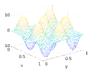
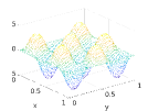
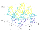
Figure 2: Target $y_{d}$ (left), optimal state $y$ (middle), and optimal control $u$ (right) computed for $b=10$, $\nu=10^{-7}$ and $\beta=10^{-2}$.

To study the efficiency and the robustness of the proposed numerical framework, we test the nonlinearly preconditioned Newton for several values of parameters $\nu$, $\beta$, $\bar{u}$, $b$ and $q$, and compare the obtained number of iterations with the ones performed by a (damped) semismooth Newton applied directly to (3). Moreover, to improve the robustness of our preconditioned Newton method, we implemented a continuation procedure with respect to the regularization parameter $\nu$. This parameter is reduced over successive iterations according to the rule $\nu_{k+1}=\max\{\nu_{k}/4\,,\,\nu\}$, where $\nu_{1}=10^{-1}$ and $\nu$ is the desired final value; see, e.g., CiaramellaNewton for convergence results about similar continuation procedures. We initialize the three methods by randomly chosen vectors. The number of iterations performed by both methods to reach a tolerance of $10^{-8}$ are reported in Tab. 1, where the symbol $\times$ indicates non-convergence. From these results, it is clear that if the preconditioned Newton converges, then it outperforms the semismooth Newton applied directly to the full system (3). However, the preconditioned Newton does not always converge due to the lack of damping. Choosing a large Robin parameter improves the robustness of the iterations, but it is not capable of fully resolving this issue. The continuation strategy, on the other hand, always leads to convergence with an iteration count comparable (for moderate values of $\nu$) or much lower (for small values of $\nu$) than that of the semismooth Newton method.

To better gauge the computational cost of the continuation strategy, we show the total number of inner iterations required by ‘pure’ preconditioned Newton versus the one with continuation in Tab. 2. The reported numbers are computed as $\sum_{k}\max_{j=1,2}{\rm it}_{j,k}$, where $k$ is the iteration count and ${\rm it}_{j,k}$, $j=1,2$, are the number of inner iterations required by the two subdomain solves performed at the $k$th outer iteration. (The max accounts for the fact that the two subdomain problems are supposed to be solved in parallel.) The results show that the continuation procedure actually reduces the total number of inner iterations for the most part, except for some very easy cases, such as $\beta=b=0$, $\bar{u}=\infty$ (where the problem is in fact linear).

Finally, we remark that the GMRES iteration count is generally 5–30 times lower for the preconditioned Newton methods than for semi-smooth Newton applied directly to (3). This is because the Jacobians of preconditioned Newton naturally include optimized Schwarz preconditioning, whereas semismooth Newton on (3) requires additional preconditioning in order to be competitive. All these numerical observation show clearly the efficiency of the proposed computational framework.

			$\bar{u}=10^{3}$			$\bar{u}=\infty$
	$q$	$b$	$\nu=10^{-3}$	$\nu=10^{-5}$	$\nu=10^{-7}$	$\nu=10^{-3}$	$\nu=10^{-5}$	$\nu=10^{-7}$
	1	0	4 - 5 - 2	6 - 9 - 14	$\times$ - 11 - 47	3 - 5 - 2	3 - 9 - 2	3 - 11 - 3
	10	0	4 - 5 - 2	6 - 9 - 14	7 - 11 - 47	3 - 5 - 2	3 - 8 - 2	3 - 11 - 3
$\beta=0$	100	0	3 - 5 - 2	6 - 9 - 14	$\times$ - 11 - 47	3 - 5 - 2	3 - 9 - 2	3 - 12 - 3
	1	10	$\times$ - 6 - 4	$\times$ - 10 - 8	$\times$ - 12 - 23	6 - 6 - 4	$\times$ - 10 - 23	$\times$ - 15 - $\times$
	10	10	6 - 6 - 4	$\times$ - 10 - 8	9 - 12 - 23	6 - 6 - 4	$\times$ - 10 - 23	$\times$ - 14 - $\times$
	100	10	4 - 6 - 4	6 - 10 - 8	$\times$ - 13 - 23	4 - 6 - 4	6 - 10 - 23	$\times$ - 13 - $\times$
	1	0	5 - 5 - 3	7 - 9 - 7	3 - 12 - 35	4 - 5 - 3	5 - 9 - 5	$\times$ - 12 - 8
	10	0	5 - 5 - 3	5 - 9 - 7	2 - 11 - 35	4 - 5 - 3	4 - 9 - 5	$\times$ - 12 - 8
$\beta=10^{-2}$	100	0	4 - 5 - 3	6 - 10 - 7	9 - 12 - 35	4 - 5 - 3	5 - 9 - 5	$\times$ - 12 - 8
	1	10	$\times$ - 6 - 4	$\times$ - 11 - 9	$\times$ - 12 - 37	6 - 6 - 4	$\times$ - 10 - 35	$\times$ - 13 - $\times$
	10	10	5 - 6 - 4	$\times$ - 11 - 9	$\times$ - 13 - 37	6 - 6 - 4	$\times$ - 10 - 35	$\times$ - 14 - $\times$
	100	10	4 - 6 - 4	6 - 11 - 9	11 - 13 - 37	4 - 6 - 4	6 - 10 - 35	$\times$ - 13 - $\times$

Table 1: Two subdomains: outer iterations of preconditioned Newton (left value), preconditioned Newton with continuation (middle value) and semismooth Newton applied to the original problem (right value).

			$\bar{u}=10^{3}$			$\bar{u}=\infty$
	$q$	$b$	$\nu=10^{-3}$	$\nu=10^{-5}$	$\nu=10^{-7}$	$\nu=10^{-3}$	$\nu=10^{-5}$	$\nu=10^{-7}$
	1	0	6 - 5	31 - 12	$\times$ - 18	2 - 5	3 - 8	3 - 11
	10	0	5 - 5	26 - 11	96 - 19	2 - 5	3 - 8	3 - 11
$\beta=0$	100	0	2 - 5	18 - 13	$\times$ - 19	2 - 5	2 - 8	3 - 11
	1	10	$\times$ - 17	$\times$ - 35	$\times$ - 47	27 - 17	$\times$ - 34	$\times$ - 60
	10	10	21 - 14	$\times$ - 31	103 - 43	21 - 14	$\times$ - 32	$\times$ - 53
	100	10	8 - 14	26 - 32	$\times$ - 43	8 - 14	45 - 30	$\times$ - 47
	1	0	13 - 8	32 - 16	84 - 25	8 - 8	10 - 14	$\times$ - 25
	10	0	10 - 8	22 - 17	33 - 23	7 - 8	11 - 15	$\times$ - 24
$\beta=10^{-2}$	100	0	7 - 6	15 - 15	104 - 20	7 - 6	12 - 13	$\times$ - 22
	1	10	$\times$ - 17	$\times$ - 33	$\times$ - 45	28 - 17	$\times$ - 32	$\times$ - 47
	10	10	20 - 14	$\times$ - 33	$\times$ - 48	20 - 14	$\times$ - 30	$\times$ - 46
	100	10	10 - 14	23 - 30	125 - 44	10 - 14	40 - 26	$\times$ - 44

Table 2: Two subdomains: total number of inner iterations of preconditioned Newton (left value) and preconditioned Newton with continuation (right value).

Let us now consider a multiple subdomain case. In this case, the discretization mesh is refined to have $101$ interior points on each edge of $\Omega$. We then repeat the experiments presented above, but we fix $q=100$ and consider different numbers of subdomains, namely $N=4,8,16$. The results of these experiments are reported in Tab. 3 and 4, where the number of iterations of the preconditioned Newton method (without and with continuation) are compared to those of the semismooth Newton method applied to (3). These results show that the preconditioned Newton methods are robust against the number of subdomains, even though the size of the subdomains decreases; see Chaouqui2018 ; CiaramellaGander for related scalability discussions. Moreover, as for the two-subdomain case, the continuation procedure exhibits convergence in all cases.

			$\bar{u}=10^{3}$			$\bar{u}=\infty$
	$N$	$b$	$\nu=10^{-3}$	$\nu=10^{-5}$	$\nu=10^{-7}$	$\nu=10^{-3}$	$\nu=10^{-5}$	$\nu=10^{-7}$
	4	0	3 - 5 - 2	7 - 10 - 7	$\times$ - 11 - 27	3 - 5 - 2	3 - 9 - 2	3 - 11 - 3
	8	0	3 - 5 - 2	$\times$ - 10 - 7	$\times$ - 11 - 27	3 - 5 - 2	3 - 9 - 2	3 - 12 - 3
$\beta=0$	16	0	3 - 5 - 2	$\times$ - 10 - 7	$\times$ - 11 - 27	3 - 5 - 2	3 - 9 - 2	3 - 12 - 3
	4	10	4 - 6 - 4	7 - 11 - 7	10 - 14 - 21	4 - 6 - 4	6 - 10 - 10	$\times$ - 13 - $\times$
	8	10	4 - 6 - 4	$\times$ - 11 - 7	$\times$ - 14 - 21	5 - 6 - 4	6 - 10 - 10	$\times$ - 13 - $\times$
	16	10	4 - 6 - 4	9 - 11 - 7	$\times$ - 14 - 21	4 - 6 - 4	6 - 10 - 10	$\times$ - 13 - $\times$
	4	0	4 - 6 - 3	6 - 10 - 6	11 - 12 - 15	4 - 6 - 3	5 - 9 - 5	8 - 13 - 9
	8	0	4 - 6 - 3	$\times$ - 10 - 6	$\times$ - 12 - 15	4 - 6 - 3	6 - 9 - 5	8 - 13 - 9
$\beta=10^{-2}$	16	0	4 - 6 - 3	8 - 10 - 6	$\times$ - 12 - 15	4 - 6 - 3	6 - 9 - 5	10 - 13 - 9
	4	10	4 - 6 - 4	6 - 10 - 6	12 - 13 - 17	4 - 6 - 4	6 - 10 - 11	$\times$ - 13 - $\times$
	8	10	4 - 6 - 4	$\times$ - 11 - 6	$\times$ - 16 - 17	5 - 6 - 4	7 - 10 - 11	$\times$ - 13 - $\times$
	16	10	4 - 6 - 4	8 - 11 - 6	$\times$ - 18 - 17	4 - 6 - 4	8 - 10 - 11	$\times$ - 14 - $\times$

Table 3: Multiple subdomains: outer iterations of preconditioned Newton (left value), preconditioned Newton with continuation (middle value) and semismooth Newton applied to the original system (right value).

			$\bar{u}=10^{3}$			$\bar{u}=\infty$
	$N$	$b$	$\nu=10^{-3}$	$\nu=10^{-5}$	$\nu=10^{-7}$	$\nu=10^{-3}$	$\nu=10^{-5}$	$\nu=10^{-7}$
	4	0	2 - 5	21 - 15	$\times$ - 18	2 - 5	2 - 8	3 - 11
	8	0	2 - 5	$\times$ - 12	$\times$ - 15	2 - 5	2 - 8	3 - 11
$\beta=0$	16	0	4 - 5	$\times$ - 13	$\times$ - 15	2 - 5	2 - 8	3 - 11
	4	10	8 - 12	32 - 30	75 - 47	9 - 12	31 - 28	$\times$ - 45
	8	10	8 - 11	$\times$ - 27	$\times$ - 44	8 - 11	28 - 26	$\times$ - 42
	16	10	7 - 11	29 - 27	$\times$ - 36	7 - 11	27 - 24	$\times$ - 39
	4	0	7 - 8	17 - 19	61 - 22	7 - 8	11 - 15	44 - 29
	8	0	7 - 7	$\times$ - 15	$\times$ - 19	7 - 7	13 - 14	35 - 26
$\beta=10^{-2}$	16	0	6 - 6	14 - 15	$\times$ - 18	5 - 6	9 - 12	32 - 24
	4	10	10 - 13	23 - 27	106 - 44	10 - 13	31 - 27	$\times$ - 43
	8	10	10 - 11	$\times$ - 27	$\times$ - 46	9 - 11	30 - 26	$\times$ - 42
	16	10	8 - 11	24 - 27	$\times$ - 44	8 - 11	30 - 23	$\times$ - 38

Table 4: Multiple subdomains: total number of inner iterations of preconditioned Newton (left value) and preconditioned Newton with continuation (right value).

4 Further discussion and conclusion

This short manuscript represents a proof of concept for using domain decomposition-based nonlinear preconditioning to efficiently solve nonlinear, nonsmooth optimal control problems governed by elliptic equations. However, several theoretical and numerical issues must be addressed as part of a complete development of these techniques. From a theoretical point of view, to establish concrete convergence results based on classical semismooth Newton theory, it is crucial to study the (semismoothness) properties of the subdomain solution maps $\mathcal{S}_{j}$, which are implicit function of semi-smooth maps. Another crucial point is the proof of well-posedness of the (preconditioned) Newton linear system. From a domain decomposition perspective, more general decompositions (including cross points) must be considered. Finally, a detailed analysis of the scalability of the GMRES iterations is necessary.

References

- [1] E. Casas, R. Herzog, and G. Wachsmuth. Optimality conditions and error analysis of semilinear elliptic control problems with L1 cost functional. SIAM J. Optim., 22(3):795–820, 2012.
- [2] F. Chaouqui, G. Ciaramella, M. J. Gander, and T. Vanzan. On the scalability of classical one-level domain-decomposition methods. Vietnam Journal of Mathematics, 46(4):1053–1088, 2018.
- [3] G. Ciaramella, A. Borzi, G. Dirr, and D. Wachsmuth. Newton methods for the optimal control of closed quantum spin systems. SIAM J. Sci. Comp., 37(1):A319–A346, 2015.
- [4] G. Ciaramella and M. J. Gander. Analysis of the parallel Schwarz method for growing chains of fixed-sized subdomains: Part I. SIAM J. Numer. Anal., 55(3):1330–1356, 2017.
- [5] M. J. Gander. Optimized Schwarz methods. SIAM J. Numer. Anal., 44(2):699–731, 2006.
- [6] G. Stadler. Elliptic optimal control problems with L1-control cost and applications for the placement of control devices. Comput. Optim.Appl., 44(2):159–181, 2009.
- [7] F. Tröltzsch. Optimal Control of Partial Differential Equations: Theory, Methods, and Applications. Graduate Studies in Mathematics. American Mathematical Society, 2010.