Optimizer Fusion: Efficient Training
with Better Locality and Parallelism

Abstract

Machine learning frameworks adopt iterative optimizers to train neural networks. Conventional eager execution separates the updating of trainable parameters from forward and backward computations. However, this approach introduces nontrivial training time overhead due to the lack of data locality and computation parallelism. In this work, we propose to fuse the optimizer with forward or backward computation to better leverage locality and parallelism during training. By reordering the forward computation, gradient calculation, and parameter updating, our proposed method improves the efficiency of iterative optimizers. Experimental results demonstrate that we can achieve an up to $20\%$ training time reduction on various configurations. Since our methods do not alter the optimizer algorithm, they can be used as a general “plug-in” technique to the training process.

1 Introduction

Iterative methods, such as stochastic gradient descent and its variants, are the mainstream optimization algorithms for training machine learning models. In these methods, learnable parameters are updated step by step until the stopping criterion is met. Many commonly used iterative optimization methods are implemented in popular machine learning frameworks, e.g. PyTorch Paszke et al. (2019), TensorFlow Abadi et al. (2015), MXNet Chen et al. (2015), and Chainer Tokui et al. (2019).

One critical component of these machine learning frameworks is automatic differentiation, which computes the gradients for all operations on tensors. The smooth integration between the optimization kernel and automatic differentiation makes the training more accessible and boosts the popularization of these frameworks in the machine learning community.

Eager execution is widely adopted in these frameworks for its flexibility. It usually decouples the forward propagation, gradient computation, and parameter updating into three separate stages. In each iteration, forward computation is first performed. Gradients respective to the loss function are then calculated for all learnable parameters. Finally, learnable parameters are updated by a specified optimizer. Although this implementation has an intuitive and transparent procedure, the learnable parameters and their gradients are read and written several times throughout one training iteration, such that these data are not efficiently reused. Moreover, gradient updating is enforced to be after the gradient computation based on the implicit control dependency, leading to lower parallelism in the program execution. In short, there is potential for higher training efficiency with better locality and parallelism in the eager execution.

In this work, we propose two methods forward-fusion and backward-fusion, which reorder the forward computation, gradient calculation, and parameter updating to accelerate the training process in eager execution. Our proposed methods fuse the optimizer with forward or backward computation to better leverage locality and parallelism. The backward-fusion method, motivated by the static computational graph compilation, where the optimizer is fused with gradient computation, updates the parameters as early as possible. For example, the optimizer in TensorFlow supports different gating gradients configurations. The forward-fusion method fuses the parameter updates with the next forward computation such that learnable parameters are updated as late as possible. Like back-propagation through time (BPTT) Werbos (1990), the forward-fusion method expands the training process through iterations and uncovers a novel perspective of acceleration.

We summarize the advantages of our methods as follows.

• Efficient. Our framework can increase the training speed by up to $20\%$.

• General. Our methods are orthogonal to other optimization methods and do not affect the training results. Thus, they can be applied in the training process of various machine learning tasks with different optimizers. We keep all the features of the eager execution.

• Simple. It is easy to replace the old training routines with our new methods. Users can accelerate their imperative training with little engineering effort.

2 Background

Static and Dynamic Computational Graphs. The training process can be viewed as a computational graph. Figure 1(a) demonstrates the corresponding computation dependency for a three-layer neural network, where nodes represent tensor computations, and directed edges stand for data dependencies. Any topological order of this graph is a valid computation order.

Generally, there are two paradigms for tensor computations in machine learning frameworks. The first category of framework compiles a model as a static (symbolic) computational graph and executes the graph with all the neural network information. For example, TensorFlow 1.X follows this routine by default Abadi et al. (2015), which requires a pre-compiled graph before execution. The other category of framework works in the eager (imperative) mode, which immediately executes the newly-encountered computation node and incrementally builds a dynamic computational graph. At each step, a computation node is appended to the current computational graph. PyTorch Paszke et al. (2019) and TensorFlow 2.X Abadi et al. (2015) both run in eager mode by default, enabling users to develop machine learning models more easily and quickly. The eager mode also enables the efficient development of non-stationary neural architectures. These two categories of frameworks are both widely used in the community. For example, in the MLPerf training benchmark Mattson et al. (2020), both static and eager modes are used and achieve the state of the art performance.

Graph Optimization. Engineers and practitioners in machine learning frameworks have proposed and implemented many graph optimizers, such as TensorFlow’s Grappler Larsen & Shpeisman (2019) and TASO Jia et al. (2019). The backward-fusion method has been considered in some of them. However, to our best knowledge, existing graph optimizers need the information of the whole computation graph, which means the optimizer fusion can only be used for (1) the static computation or (2) the mixture of static and dynamic execution. In most machine learning frameworks, the purely eager mode still separates forward computation, backward pass, and parameter updating into three stages, with the topological order shown in Figure 1(b). The framework will first execute the forward and backward computation to obtain gradients. Then learnable parameters will be updated following the optimizer. This imperative nature allows users to monitor the training process at the cost of low efficiency. For instance, the TensorFlow eager execution follows this routine. 

We enable the backward-fusion method in purely eager mode. The forward-fusion method also uncovers a novel perspective, where graphs can be optimized across iterations.

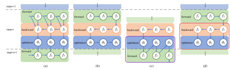
Figure 1: (a) Data dependency graph. (b) Baseline method. (c) Forward-fusion. (d) Backward-fusion. $\theta_{i}$ represents the trainable parameters in the layer $f_{i}$.

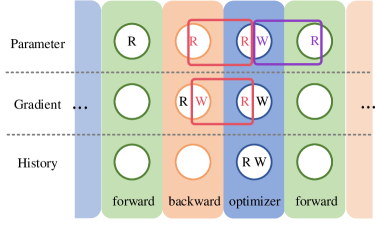
Figure 2: Memory transactions and data locality in the training process. R and W represent memory read and write, respectively. History means parameter history needed in the optimizer, e.g., momentum. Red and purple frames represent locality improvement in backward-fusion and forward-fusion, respectively.

3 Methods

Figure 1 shows the baseline method, and the proposed forward-fusion and backward-fusion methods.

Baseline. Figure 2 illustrates the memory transactions and the locality that can be leveraged in the training process. Trainable parameters are read during forward and backward computations and updated by the optimizer. Gradients are accumulated during the backward pass. Finally, they are read and reset by the optimizer. History represents the parameter history, such as momentum. The optimizer records and updates the parameter history.

All these memory reads and writes are separated by forward, backward, and optimizer stages. The memory capacity is usually not large enough to hold all the data through the training iteration. The data locality between the optimizer and its adjacent forward or backward computations is lost. If we access the same set of data repetitively before the data is flushed, we can shorten the time of memory access and thus accelerate the training process.

Also, the baseline method does not take advantage of the parallelism between backward computations and parameter updating. While updating a group of parameters, we can continue the back-propagation to compute gradients for other independent parameters at the same time, which offers another opportunity for better parallelism in the training process.

Forward-Fusion. One approach is to fuse the optimizer with the forward computation in the next iteration. The next forward pass can occur in either a training or an evaluation process. Each trainable parameter will be updated as late as possible. This lazy update strategy is named forward-fusion. The proposed method can be applied in all the iterative methods, including the optimizer that needs global information.

The memory write operation during parameter updating can be merged with the next read, such that in the next forward computation, the cached parameter can be quickly accessed with low latency. The purple frame in Figure 2 illustrates this improvement.

Unlike current machine learning frameworks, which ignore the optimization potential across different iterations, we find the opportunity between adjacent training steps. Similar to back-propagation through time Werbos (1990), the training process of a feed-forward neural network training can also be expanded through iterations. This perspective is a new direction for accelerating the machine learning models embracing both static and dynamic computational graphs.

Backward-Fusion. Another approach is to fuse the optimization computation with gradient computation in the backward pass, as shown in Figure 1(d). This method applies gradients to parameters as early as possible, so that the memory access can be merged to increase the locality, as shown in the red frame in Figure 2. Specifically, two consecutive parameter reads in the backward pass and optimizer can be merged, such that the second read during the optimization step can be accelerated as it can be cached in the local storage. Gradient accumulation in the backward computation can be merged with the memory read in the optimizer. Thus, the updated gradients can be efficiently accessed in the local storage to shorten the memory access time.

Moreover, this method improves training efficiency as it parallelizes the parameter updating and gradient back-propagation. This method applies to most optimizers that do not require global information of trainable parameters, as this fusion strategy assumes the update of $\theta_{i}$ is decoupled with other parameters $\theta_{j}(i\neq j)$. In the view of the computational graph, the depths of the directed graphs shown in Figures 1(b), (d) are $3n$ and $2n+1$, respectively, where $n$ is the number of layers in the neural network. Thus, the backward-fusion method also provides extra parallelism.

Table 1 summarizes the characteristics of our proposed methods.

Table 1: Comparison among three methods: locality, parallelism, and global information.

Method Locality Parallelism Global Info. baseline $\times$ $\times$ $\checkmark$ forward-fusion $\checkmark$ $\times$ $\checkmark$ backward-fusion $\checkmark$ $\checkmark$ $\times$

4 Experiments

Figure 3: Training time breakdown of MobileNetV2 with mini-batch size 32. FF, BF are short for forward-fusion, backward-fusion.

Figure 3 shows the time breakdown of one training iteration of MobileNetV2 Sandler et al. (2018) with a mini-batch size of 32. After we fuse the optimizer with backward computation, the execution time of backward increases by $3.32$ ms, much smaller than the original optimizer execution time ($16.70$ ms). In this example, our forward-fusion and backward-fusion improve the training throughput by $12\%$ and $16\%$, respectively.

We show more results in Appendix C.

5 Conclusions

Conventional eager execution in machine learning frameworks separate the updating of trainable parameters from forward and backward computations. In this paper, we propose two methods forward-fusion and backward-fusion to better leverage the locality and parallelism during training. We reorder the forward computation, gradient calculation, and parameter updating, so that our proposed methods improve the efficiency of iterative optimizers. Experimental results demonstrate the effectiveness and efficiency of our methods across various configurations. Our forward-fusion method opens a new perspective of performance optimization for machine learning frameworks.

Appendix A Extended Related Work

Iterative Optimization Methods. An iterative optimization algorithm starts from an initial guess and derives a sequence of improving approximate solutions. Algorithm 1 is the general structure of iterative optimization methods for unconstrained problems. The step vector $\Delta\theta$ is computed from the optimizer policy $\pi$. The policy $\pi$ is the only difference across different optimization algorithms. The commonly used gradient-based methods use policies that depend on the first-order derivative information.

For instance, the policies demonstrated in Equations (1), (2), and (3) are used in the gradient descent, gradient descent with momentum, Newton’s method, respectively,

$$\pi_{1}=-\eta\nabla f(\theta^{(t-1)})$$ (1)

$$\pi_{2}=-\eta\sum_{\tau=0}^{t-1}\alpha^{t-\tau-1}\nabla f(\theta^{(\tau)})$$ (2)

$$\pi_{3}=-\eta\nabla^{2}f(\theta^{(t-1)})^{-1}\nabla f(\theta^{(t-1)})$$ (3)

where $\eta$ represents the step size, $\alpha$ denotes the momentum decay factor.

Algorithm 1 Optimization algorithms in general form

  Input: objective function $f$

  Initialize the starting point $\theta^{(0)}$

  for $t=1,2,...$ do

     if stopping criterion is met then

        return $\theta^{(t-1)}$

     end if

     $\Delta\theta=\pi(f,{\theta^{(0)},\theta^{(1)},...,\theta^{(t-1)}})$

     $\theta^{(t)}=\theta^{(t-1)}+\Delta\theta$

  end for

Locality and Parallelism. Fruitful hardware-aware techniques in machine learning have been proposed to accelerate the training process, especially on graphics processing units (GPUs). Generally speaking, common approaches include accelerating the kernel computations Li et al. (2019), mixed precision training Micikevicius et al. (2018) , fusing kernels and operations Wu et al. (2012), and exploring efficient network architecture Gong et al. (2019). Data locality and computation parallelism are two critical aspects of performance optimization.

The work of fused-layer CNN accelerators Alwani et al. (2016) proposes a new architecture for inference by fusing the convolution layers. It decomposes the inputs to the convolution layers into tiles and propagates one tile through multiple layers. With reduced memory access and better cache utilization, the inference speed is improved. Lym et al. Lym et al. (2019) design a new scheme to eliminate most memory accesses in neural network training by reordering the computation within a mini-batch for better data locality. Apex for PyTorch  uses fused optimizers, which launch one kernel for the element-wise operations.

From a perspective different from the aforementioned previous works, we explore the parallelism and locality across the gradient computation and the optimizer. We also uncover the potential of acceleration across iterations.

Appendix B Extended Method

B.1 Forward-fusion

Algorithm 2 shows the pipeline of this method. It is possible that a layer is used many times, i.e., $f_{i}=f_{j},i\neq j$ in Algorithm  2. We use a flag updated to ensure that the parameter is updated only once no matter how many times the corresponding layer is used. This method can also be applied when we need to manipulate the gradients based on global information Reddi et al. (2018). For instance, this method is suitable when we would like to clip the gradients by their global norm.

Algorithm 2 Forward-fusion

  Input: topologically sorted operator array $\{f_{i}\}_{i=1}^{n}$

  for $i=1,2,...,n$ do

     if $f_{i}$.updated is False then

        for each trainable parameters $\theta$ in $f_{i}$ do

           execute optimizer of $\theta$

        end for

        $f_{i}$.updated $\leftarrow$ True

     end if

     execute $f_{i}$

  end for

  for $i=n,n-1,...,1$ do

     execute backward pass of $f_{i}$

     accumulate gradients for all trainable parameters

     $f_{i}$.updated $\leftarrow$ False

  end for

B.2 Backward-fusion

Algorithm 3 demonstrates the computational flow. After calculating the gradient of $\theta_{i}$, we apply the gradient in the optimizer directly. At the same time, we resume the backward computation for node $f_{i-1}$. For each parameter $\theta_{i}$, we record the number of its usage in the forward pass as $\theta_{i}$.count. Correspondingly, we will update it until its gradient is accumulated for all its usage in the forward pass.

Algorithm 3 Backward-fusion

  Input: topologically sorted operator array $\{f_{i}\}_{i=1}^{n}$

  for $i=1,2,...,n$ do

     execute $f_{i}$

     for each trainable parameters $\theta$ in $f_{i}$ do

        $\theta$.count $\leftarrow$ $\theta$.count $+1$

     end for

  end for

  for $i=n,n-1,...,1$ do

     execute backward pass of $f_{i}$

     for each trainable parameters $\theta$ in $f_{i}$ do

        accumulate gradient of $\theta$

        $\theta$.count $\leftarrow$ $\theta$.count $-1$

        if $\theta$.count is 0 then

           execute optimizer of $\theta$

        end if

     end for

  end for

Applying gradients directly on the parameters may induce race conditions. For instance, for a multiplication operator $f(\theta,x)=\theta x$, $\partial f/\partial\theta=x,\partial f/\partial x=\theta$. $\partial f/\partial x$ depends on the original parameter $\theta^{(t)}$, instead of the updated parameter $\theta^{(t+1)}$. Therefore, we must carefully tackle this dependency. Specifically, for a trainable parameter $\theta$, we will update it in-place to obtain $\theta^{(t+1)}$ when the following two conditions are both satisfied: (1) its gradient $\partial L/\partial\theta$ is calculated, and (2) there is no other dependency on the old value $\theta^{(t)}$.

Appendix C Experiment details

We evaluate the effectiveness and efficiency of our proposed methods with various mini-batch sizes, optimizers, machine learning models and benchmarks, machines (GPUs) and frameworks.

C.1 Experimental Settings

Unless stated otherwise, we conduct experiments on the eager execution in PyTorch 1.6.0. We implement the proposed methods in the PyTorch front-end using hooks. A toy example is provided in the supplementary file. The training process runs on a Linux server with Intel Core i9-7900X CPU and a NVIDIA TITAN Xp GPU based on Pascal architecture. We use Adam Kingma & Ba (2015) with weight decay to do the training on image classification using the ImageNet dataset Deng et al. (2009). All the tensor computations occur on 1 GPU with single-precision floating-point (float32) datatype.

We report the mean of 100 training iterations.

C.2 Various Mini-batch Sizes

Figure 4: The absolute execution time saved by our methods on MobileNetV2 with different mini-batch sizes.

(a)

(b)

(c)

(d)

(e)

(f)

Figure 5: Training speedup with various mini-batch sizes on different benchmarks.

Compared with the baseline method, our two methods have the overhead of control as shown in Algorithms 2 and 3. When a small mini-batch size is used, the overhead of the control flow will exceed the benefits of better locality and parallelism, which makes our framework slower than the baseline. As the mini-batch size increases, the overhead becomes negligible compared with the computation time. The effectiveness of our proposed methods requires this overhead to be amortized by an appropriate mini-batch size.

When the mini-batch size is large enough such that we reach the performance roofline of the GPUs, the computation time of forward and backward pass is approximately linear to the mini-batch size. On the other hand, the optimizer execution time is independent of the mini-batch size. Therefore, the absolute training time saved by our methods is independent of the mini-batch size, as shown in Figure 4. The relative speedup will decrease as the mini-batch size grows, as demonstrated in Figure 5.

The discussion above can also be formulated in the following equation. The theoretical speedup of the training process is

$$s=\frac{bt_{grad}+t_{opt}}{bt_{grad}+t_{opt}-t_{saved}}$$

where $b$ represents the mini-batch size, $t_{grad}$ is the time of forward and backward computation per mini-batch size, $t_{opt}$ is the execution time of optimizer, and $t_{saved}$ stands for the absolute saved time on the optimizer with our methods.

Both forward-fusion and backward-fusion methods leverage the locality of the trainable parameters. However, only the backward-fusion method takes advantage of the parallelism between the gradient computation and optimizer. When the mini-batch size is small, the GPU is not fully utilized. Thus, the parallelism exploited by backward-fusion will accelerate the training significantly compared with forward-fusion. As mini-batch sizes grow, the gradient computation dominates the GPU utilization. Therefore, the execution time of these two methods converges at large mini-batch sizes, as illustrated in Figure 5.

C.3 Various Models and Optimizers

We sweep the mini-batch size for different models He et al. (2016); Huang et al. (2017); Sandler et al. (2018); Simonyan & Zisserman (2015); Ioffe & Szegedy (2015) as shown in Figure 5. Figure 6 demonstrates the relationship between the parameter size and speedup across different models. The smaller the average number of parameters per layer, the more locality we can leverage so that our methods can achieve higher training speed. This explains why the VGG19_BN is hardly accelerated while the MobileNetV2 has the most significant improvement. Currently, the models targeting at edge devices usually contain fewer parameters, whose training will benefit more from our methods.

Figure 6: The speedup trend among different models with a mini-batch size of 32. In average, fewer parameters per layer leads to higher speedup.

Figure 7: Comparison among various optimizers on MobileNetV2 with a mini-batch size of 32. Weight decay is applied in all these methods unless specified. The horizontal axis represents the ratio of the optimizer time to a whole iteration time.

Various optimizers used in machine learning frameworks can benefit from our proposed methods. Figure 7 shows an increasing trend between speedup and the runtime ratio of different optimizers Zeiler (2012); Kingma & Ba (2015); Duchi et al. (2011). The horizontal axis is the ratio of the optimizer runtime to a whole iteration runtime. The more runtime-costly the optimizer, the higher speedup we can achieve.

C.4 Various Machines and Benchmarks

Table 2: Training results on MobileNetV2 with a mini-batch size of 32 across various machines.

CPU	GPU	baseline	forward-fusion	backward-fusion	forward-fusion	backward-fusion
		runtime (ms)	runtime (ms)	runtime (ms)	speedup	speedup
Core i9-7900X	TITAN Xp	98.77	84.52	82.99	1.17	1.19
Core i7-3770	GTX 1080	163.60	145.80	129.71	1.12	1.26
Core i7-8750H	GTX 1070 maxQ	174.43	157.27	158.89	1.11	1.10

Our methods are practical and efficient on various machine configurations, as shown in Table 2. The speedup depends on the cache size, the floating point operations per second (FLOPS), memory bandwidth, etc. Although the relationship is very complicated and beyond our discussion, our methods stay effective on various GPUs.

Our methods can be used in all the iterative optimization problems. Thus it can be used in almost all machine learning problems. For example, we train the Transformer (base) Vaswani et al. (2017) on the WMT English-German dataset. With a min-batch size of 256, we can achieve the speedup of $1.030$ and $1.019$ respectively using our forward-fusion and backward-fusion methods.

C.5 Mulit-GPUs

There are many training methods in distributed computation, such as distributed data parallel (DDP) training, training leveraging model parallelism. Our proposed method can be easily extended to the DDP training since the optimizer is managed in only one machine. The training speedup with DDP is similar to that on a single GPU. However, it is challenging to handle other distributed training methods, which is the future direction of this work.

References

- Abadi et al. (2015) Martín Abadi, Ashish Agarwal, Paul Barham, Eugene Brevdo, Zhifeng Chen, Craig Citro, Greg S. Corrado, Andy Davis, Jeffrey Dean, Matthieu Devin, Sanjay Ghemawat, Ian Goodfellow, Andrew Harp, Geoffrey Irving, Michael Isard, Yangqing Jia, Rafal Jozefowicz, Lukasz Kaiser, Manjunath Kudlur, Josh Levenberg, Dandelion Mané, Rajat Monga, Sherry Moore, Derek Murray, Chris Olah, Mike Schuster, Jonathon Shlens, Benoit Steiner, Ilya Sutskever, Kunal Talwar, Paul Tucker, Vincent Vanhoucke, Vijay Vasudevan, Fernanda Viégas, Oriol Vinyals, Pete Warden, Martin Wattenberg, Martin Wicke, Yuan Yu, and Xiaoqiang Zheng. TensorFlow: Large-scale machine learning on heterogeneous systems, 2015.
- Alwani et al. (2016) Manoj Alwani, Han Chen, Michael Ferdman, and Peter Milder. Fused-layer cnn accelerators. In The 49th Annual IEEE/ACM International Symposium on Microarchitecture (MICRO). IEEE Press, 2016.
- Chen et al. (2015) Tianqi Chen, Mu Li, Yutian Li, Min Lin, Naiyan Wang, Minjie Wang, Tianjun Xiao, Bing Xu, Chiyuan Zhang, and Zheng Zhang. Mxnet: A flexible and efficient machine learning library for heterogeneous distributed systems. CoRR, abs/1512.01274, 2015.
- Deng et al. (2009) J. Deng, W. Dong, R. Socher, L.-J. Li, K. Li, and L. Fei-Fei. ImageNet: A Large-Scale Hierarchical Image Database. In CVPR09, 2009.
- Duchi et al. (2011) John Duchi, Elad Hazan, and Yoram Singer. Adaptive subgradient methods for online learning and stochastic optimization. J. Mach. Learn. Res., 12:2121–2159, July 2011. ISSN 1532-4435.
- Gong et al. (2019) C. Gong, Z. Jiang, D. Wang, Y. Lin, Q. Liu, and D. Z. Pan. Mixed precision neural architecture search for energy efficient deep learning. In 2019 IEEE/ACM International Conference on Computer-Aided Design (ICCAD), pp. 1–7, Nov 2019.
- He et al. (2016) K. He, X. Zhang, S. Ren, and J. Sun. Deep residual learning for image recognition. In 2016 IEEE Conference on Computer Vision and Pattern Recognition (CVPR), pp. 770–778, June 2016.
- Huang et al. (2017) G. Huang, Z. Liu, L. v. d. Maaten, and K. Q. Weinberger. Densely connected convolutional networks. In 2017 IEEE Conference on Computer Vision and Pattern Recognition (CVPR), pp. 2261–2269, July 2017.
- Ioffe & Szegedy (2015) Sergey Ioffe and Christian Szegedy. Batch normalization: Accelerating deep network training by reducing internal covariate shift. In Proceedings of the 32nd International Conference on International Conference on Machine Learning - Volume 37, ICML’15, pp. 448–456. JMLR.org, 2015.
- Jia et al. (2019) Zhihao Jia, Oded Padon, James Thomas, Todd Warszawski, Matei Zaharia, and Alex Aiken. Taso: Optimizing deep learning computation with automatic generation of graph substitutions. In Proceedings of the 27th ACM Symposium on Operating Systems Principles, SOSP ’19, pp. 47–62, New York, NY, USA, 2019. Association for Computing Machinery. ISBN 9781450368735. doi: 10.1145/3341301.3359630. URL https://doi.org/10.1145/3341301.3359630.
- Kingma & Ba (2015) Diederik P. Kingma and Jimmy Ba. Adam: A method for stochastic optimization. In 3rd International Conference on Learning Representations, ICLR 2015, San Diego, CA, USA, May 7-9, 2015, Conference Track Proceedings, 2015.
- Larsen & Shpeisman (2019) Rasmus Munk Larsen and Tatiana Shpeisman. Tensorflow graph optimizations, 2019.
- Li et al. (2019) Xiuhong Li, Yun Liang, Shengen Yan, Liancheng Jia, and Yinghan Li. A coordinated tiling and batching framework for efficient gemm on gpus. In Proceedings of the 24th Symposium on Principles and Practice of Parallel Programming, PPoPP ’19, pp. 229–241, New York, NY, USA, 2019. Association for Computing Machinery. ISBN 9781450362252.
- Lym et al. (2019) Sangkug Lym, Armand Behroozi, Wei Wen, Ge Li, Yongkee Kwon, and Mattan Erez. Mini-batch serialization: Cnn training with inter-layer data reuse. In Proceedings of SysML, 2019.
- Mattson et al. (2020) Peter Mattson, Christine Cheng, Cody Coleman, Greg Diamos, Paulius Micikevicius, David Patterson, Hanlin Tang, Gu-Yeon Wei, Peter Bailis, Victor Bittorf, David Brooks, Dehao Chen, Debojyoti Dutta, Udit Gupta, Kim Hazelwood, Andrew Hock, Xinyuan Huang, Atsushi Ike, Bill Jia, Daniel Kang, David Kanter, Naveen Kumar, Jeffery Liao, Guokai Ma, Deepak Narayanan, Tayo Oguntebi, Gennady Pekhimenko, Lillian Pentecost, Vijay Janapa Reddi, Taylor Robie, Tom St. John, Tsuguchika Tabaru, Carole-Jean Wu, Lingjie Xu, Masafumi Yamazaki, Cliff Young, and Matei Zaharia. Mlperf training benchmark, 2020.
- Micikevicius et al. (2018) Paulius Micikevicius, Sharan Narang, Jonah Alben, Gregory F. Diamos, Erich Elsen, David García, Boris Ginsburg, Michael Houston, Oleksii Kuchaiev, Ganesh Venkatesh, and Hao Wu. Mixed precision training. In 6th International Conference on Learning Representations, ICLR, 2018.
- Paszke et al. (2019) Adam Paszke, Sam Gross, Francisco Massa, Adam Lerer, James Bradbury, Gregory Chanan, Trevor Killeen, Zeming Lin, Natalia Gimelshein, Luca Antiga, Alban Desmaison, Andreas Kopf, Edward Yang, Zachary DeVito, Martin Raison, Alykhan Tejani, Sasank Chilamkurthy, Benoit Steiner, Lu Fang, Junjie Bai, and Soumith Chintala. Pytorch: An imperative style, high-performance deep learning library. In Advances in Neural Information Processing Systems 32, pp. 8024–8035. Curran Associates, Inc., 2019.
- Reddi et al. (2018) Sashank J. Reddi, Satyen Kale, and Sanjiv Kumar. On the convergence of adam and beyond. In 6th International Conference on Learning Representations, 2018.
- Sandler et al. (2018) Mark Sandler, Andrew G. Howard, Menglong Zhu, Andrey Zhmoginov, and Liang-Chieh Chen. Mobilenetv2: Inverted residuals and linear bottlenecks. In 2018 IEEE Conference on Computer Vision and Pattern Recognition, CVPR 2018, Salt Lake City, UT, USA, June 18-22, 2018, pp. 4510–4520, 2018.
- Simonyan & Zisserman (2015) Karen Simonyan and Andrew Zisserman. Very deep convolutional networks for large-scale image recognition. In International Conference on Learning Representations, 2015.
- Tokui et al. (2019) Seiya Tokui, Ryosuke Okuta, Takuya Akiba, Yusuke Niitani, Toru Ogawa, Shunta Saito, Shuji Suzuki, Kota Uenishi, Brian Vogel, and Hiroyuki Yamazaki Vincent. Chainer: A deep learning framework for accelerating the research cycle. In Proceedings of the 25th ACM SIGKDD International Conference on Knowledge Discovery & Data Mining, pp. 2002–2011. ACM, 2019.
- Vaswani et al. (2017) Ashish Vaswani, Noam Shazeer, Niki Parmar, Jakob Uszkoreit, Llion Jones, Aidan N. Gomez, Lukasz Kaiser, and Illia Polosukhin. Attention is all you need. In Advances in Neural Information Processing Systems 30, pp. 5998–6008, 2017.
- Werbos (1990) P. J. Werbos. Backpropagation through time: what it does and how to do it. Proceedings of the IEEE, 78(10):1550–1560, Oct 1990. ISSN 1558-2256.
- Wu et al. (2012) H. Wu, G. Diamos, S. Cadambi, and S. Yalamanchili. Kernel weaver: Automatically fusing database primitives for efficient gpu computation. In 2012 45th Annual IEEE/ACM International Symposium on Microarchitecture, pp. 107–118, Dec 2012.
- Zeiler (2012) Matthew D. Zeiler. ADADELTA: an adaptive learning rate method. CoRR, abs/1212.5701, 2012.